On the local dark matter density
Abstract
Context. In 2012, we applied a three-dimensional formulation to kinematic measurements of the Galactic thick disk and derived a surprisingly low dark matter density at the solar position. This result was challenged by Bovy & Tremaine (2012, ApJ, 756, 89), who claimed that the observational data are consistent with the expected local dark matter density if a one-dimensional approach is adopted.
Aims. We aim at clarifying whether their work definitively explains our results, by analyzing the assumption at the bases of their formulation and their claim that this returns a lower limit for the local dark matter density, which is accurate within 20%.
Methods. We find that the validity of their formulation depends on the underlying mass distribution. We therefore analyze the predictions that their hypothesis casts on the radial gradient of the azimuthal velocity and compare it with observational data as a testbed for the validity of their formulation.
Results. We find that their hypothesis requires too steep a profile of , which is inconsistent with the observational data both in the Milky Way and in external galaxies. As a consequence, their results are biased and largely overestimate the mass density. Dynamical simulations also show that, contrary to their claims, low values of are compatible with a Milky Way-like potential with radially constant circular velocity. We nevertheless confirm that, according to their criticism, our assumption =0 is only an approximation. If this hypothesis is released, and the available information about in the thick disk is used, the resulting local dark matter density increases by a tiny amount, from to mM⊙ pc-3, with an upper limit of 3.5 mM⊙ pc-3. Hence, this approximation has negligible influence on our results.
Conclusions. Our analysis shows that their criticism is not a viable explanation for the inferred lack of dark matter at the solar position detected by us. More studies are required to understand these unexpected results.
Key Words.
Galaxy: kinematics and dynamics — dark matter — Galaxy: structure1 Introduction
Dark matter (DM) plays a key role in many fields of modern astrophysics, and it is recognized as a fundamental component of the Universe. Despite this general agreement, its density at the solar position () is still poorly constrained. Even recent measurements are compatible within 1 with both a null local density (Creze et al., 1998; Holmberg & Flynn, 2000, e.g.,) and with a value as high11 1 The DM density will be given in the astronomical unit mM⊙ pc-3, where 1 mM⊙ pcM⊙ pc-3=0.038 GeV cm-3. as 37 mM⊙ pc-3 (Garbari et al., 2012). The predictions of current models of spherical Galactic DM halo span the range =5–13 mM⊙ pc-3 (Olling & Merrifield, 2001; Weber & de Boer, 2010, e.g.,), but the density could be much lower in the case of a non-spherical or a more centrally concentrated distribution (Olling, 1995; Einasto, 1965; Einasto, 1968), or higher by up to a factor of two in the presence of dark substructures, such as a dark matter disk or ring (Kalberla, 2003; Read et al., 2008; Purcell et al., 2009).
Recently, Moni Bidin et al. (2012b, hereafter M12b) have proposed a new formulation to measure the dynamical mass of the Galactic disk up to large heights from the plane, by using the full three-dimensional kinematics and spatial distribution of a test stellar population. The hypotheses at the basis of their calculations are not innovative, and they were (often implicitly) assumed in most of the previous estimates. Applying this formulation to the kinematical measurements of Moni Bidin et al. (2012a, herafter M12a), Moni Bidin et al. (2010); Moni Bidin et al. (2012b) found a surprising lack of DM at the solar position ( mM⊙ pc-3), at variance with most of the one-dimensional estimates even recently proposed (Zhang et al., 2013, e.g.,). A strong effort followed their work to understand the reliability of these unexpected results.
Sanders (2012) argues, by means of numerical simulations, that 25 underestimated the gradients of the velocity dispersions with Galactic height by up to a factor of three. His work impels further investigation to derive more reliable kinematical data, but it has negligible effects on the results of 26. In fact, they obtained identical results by adopting alternative data sets, where the kinematical quantities were measured with different methods. Moreover, the mass derived with their three-dimensional formulation is largely insensitive to an isotropic change in the dispersions, because a steeper gradient of the vertical component () induces an increase in the inferred mass that is compensated by the larger negative contribution of the radial and azimuthal ones ( and , respectively).
If the vertical trend of is expressed by a linear relation
| (1) |
and we isolate the terms containing in Equation (14) of 26, their contribution to the surface density is
| (2) |
where we neglected quadratic terms in , whose contribution is smaller by one order of magnitude. With the parameter definition of 26 and the kinematical values of 25, we obtain M⊙ pc-2. Thus, enhancing by a factor of three, the DM density increases by mM⊙ pc-2. However, repeating the same exercise for the other two components, we find ( M⊙ pc. As a consequence, the increase of in response to an isotropic increase in the dispersion gradients is damped by 70%, when and are taken into account. Even enhancing the vertical gradients by a factor of three, the derived local mass density increases by only 1.5 mM⊙ pc-3. A gradient of steeper than that of the other components is required to obtain a significantly higher DM density. Figure 6 of Sanders (2012) also shows that the large underestimate claimed by the author is introduced by the offset measurements at 2.5 kpc, while in the range =2.5–4 kpc, the 25 method underestimates the dispersions by only 5%, and their gradient by 15%, both compatible with their quoted errors. This discontinuity at =2.5 kpc is not observed in the real data of 25 (see their Figure 6), where the gradients change by less than if the points at 2.5 kpc are excluded. This suggests that Sanders’ simulations did not reproduce the measurements at lower heights well and that they introduced a systematic offset not present in the measurements of 25, whose gradient estimates should be accurate within 15%.
Bovy & Tremaine (2012, hereafter BT12) also argue that 26 results are flawed. They claimed that the same data of 25 are fully consistent with the standard value mM⊙ pc-3, with a lower limit of mM⊙ pc-3, if a more classical one-dimensional approach is adopted. In this paper, we analyze the hypotheses underlying their formulation in more detail, to verify that their criticism explains the results of 26 and that this is the correct solution to the puzzle. Following 26 and 3, we use the cylindrical Galactic coordinates (), where is the Galactocentric distance, is directed in the direction of Galactic rotation, and is positive toward the north Galactic pole. The respective velocity components are ()=().

2 Bovy & Tremaine’s assumptions
Both 26 and 3 estimate the mass surface density within kpc of the Galactic plane by means of the integrated Poisson equation in cylindrical coordinates:
| (3) |
with
| (4) |
where is the gravitational constant, and and are the radial and vertical components of the force per unit mass, respectively. If in Equation (4) is expressed by means of the radial Jeans equation for a population in steady state,
| (5) |
the radial gradient of the mean azimuthal velocity is introduced in the formulation, because
| (6) |
and . This quantity is poorly known observationally, and 26 assumed at any . They referred to as the “rotational” velocity and to as the “rotation curve” henceforth. This terminology is not new in the literature (Yoachim & Dalcanton, 2005, e.g.,), but very unfortunate, because the same terms are used more often for the circular velocity . Nevertheless, their Equation (11) unambiguously stated their hypothesis. 3 exposed this source of confusion, and arguing against the 26 assumption, they removed the source of the problematic term, setting at any . This reduced the three-dimensional formulation of 26 to a one-dimensional approach, similar to the previous works (Kuijken & Gilmore, 1989; Holmberg & Flynn, 2000, e.g.,), but for the first time extended beyond 1.1 kpc from the Galactic plane. They also claim that and . The first inequality implies that their assumption returns a lower limit of , because enters with negative sign in the calculation of the surface mass density. In addition, if , the resulting estimate of is accurate within 20% (see Equation (3)). They claim that they only substitute the 26 assumption with the observationally-proven fact (Sofue et al., 2009, e.g.,), but all their calculations were actually based on the implicit assumption that up to =4 kpc. However, this equation is strictly valid only on the plane. Assuming =3.8 kpc and =3.5 kpc for the radial scale length of the thick disk mass density and velocity dispersions, respectively, they derived mM⊙ pc-3, with a slope of compatible with mM⊙ pc-3. They also argue that =2 kpc should be preferred, and they obtained mM⊙ pc-3 in this case. In this section, we analyze in more detail the 3 assumption that leads to these results.

2.1 The universality of the assumption
We first analyze the 3 claim that and . The sign of and its weight in the calculation of depend critically on the mass density distribution. 3 prove the validity of their claims at kpc for an exponential disk model with scale length =3.4 kpc and for a spherical NFW (Navarro et al., 1997) dark halo. However, alternative mass distributions lead to completely different conclusions. For example, as shown in Fig. 1, is positive up to =4 kpc for the Galactic disk model of Flynn et al. (1996) at , where is the radial scale length of the disk mass density. This condition is most likely verified at the solar position, where 8–8.5 kpc and =2–3 kpc (Jurić et al., 2008; Bovy et al., 2012b). Figure 1 also shows the trend of , which exceeds 0.2 if , i.e. if 2.7 kpc.
In Fig. 2 we show the trend of at kpc for a family of Miyamoto-Nagai (MN) disk models
| (7) |
(Miyamoto & Nagai, 1975) with =0.3 kpc and total mass M⊙. The figure shows that is positive up to =3.5 kpc for the MN disk with =4 kpc used by Qu et al. (2011) and Bovy et al. (2012b) to model the Galactic disk. More in general, up to =4 kpc for a MN disk with 4 kpc. The parameter must be increased to 0.63 if we want at in the whole range =0–4 kpc.
The sign of and its incidence in Equation (3) depend on the relative weight of the individual mass components, due to the additive property of the potential. A spherical extended feature such as a DM halo gives a negative contribution, as shown for example in Fig. 2 for a NFW dark halo with =8 mM⊙ pc-3. If the Galactic disk is approximated by the aforementioned MN model with =4, the presence of such a dark halo is required to have up to =4 kpc.
It must be considered that, when is positive and neglected, the total mass is overestimated, leading to a larger overestimate of , because the spurious excess of visible mass is ascribed to a higher DM density. For example, if =5 mM⊙ pc-3, a mass overestimate of 20% at =2.5 kpc would increase the derived to 8.5 mM⊙ pc-3, thus overestimating the DM density by 70%.

In conclusion, our counterexamples show that is not negative and negligible for any Galactic mass model. As a consequence, the 3 formulation is not generally valid. It is a good approximation if the underlying mass distribution is close to the Galactic models implicitly assumed, but if it differs, the resulting estimate is not necessarily a lower limit to , nor is it accurate within 20%. Such implicit assumptions should obviously be avoided in a formulation aimed at measuring the local mass density itself.
2.2 Tests of the validity of the assumption
Given the results of the previous section, we test the 3 assumption here, to verify that their formulation is coincidentally reliable in the specific case under study. The hypothesis requires at any . When is expressed by means of Equation (5), this translates to:
| (8) |
with
| (9) |
where we assumed a mass density distribution described by a double exponential law ( and an exponential radial decay of the velocity dispersions with scale length . Both these assumptions were discussed, justified, and adopted by 3 and 26.
Equation (8) must be satisfied if the 3 hypothesis is correct. 3 claim a good match between the predictions on obtained from this equation and the observational results of Casetti-Dinescu et al. (2011, hereafter CD11). Here we study those predictions in more detail, re-analyze this comparison, and extend it to additional data sets. We assume =3.8 kpc (26; 3) and a circular velocity at the solar position km s-1 (Salucci et al., 2010), which is indistinguishable from 220 km s-1 of 3 for our purposes, but more compatible with the assumed solar Galactocentric distance =8 kpc (Kerr & Lynden-Bell, 1986; Reid et al., 1999). Following the results of Sanders (2012) discussed in Sect. 1, we increase the velocity dispersions of 25 by 5%, and their vertical gradient by 15%, although this correction has negligible effects on the results.
In Fig. 3, we show the expectations for obtained by inserting in Equation (8) the kinematical results of 25 (their Equations (3) to (5), with km s-1) and 5 (their Table 1, with km s-1), with from 26 (compatible with both data sets, see 26). The hypothesis requires high values of , and its steep increase with . Assuming =3.8 kpc and =0.9 kpc, it grows from 10 km s-1 kpc-1 at =1 kpc to 45 km s-1 kpc-1 at =4 kpc. Assuming =2 kpc, =3.5 kpc, and =0.7 kpc, as preferred by 3, increases even more, up to 80 km s-1 kpc-1 at =4 kpc. In other words, the 3 assumption requires that the thick disk rotation increases rapidly with distance from the Galactic center and much more rapidly at larger Galactic heights. For any parameter set, the radial gradient of is six to eight times higher at =4 kpc than on the Galactic plane. Thus, while the thick disk rotation decreases with distance from the plane by km s-1 kpc-1 at the solar position (Majewski, 1992; Chiba & Beers, 2000; Girard et al., 2006, e.g.,), this vertical shear would disappear within 3 kpc of the Sun (11 kpc), where the stars at =4 kpc would be corotating with those on the plane. This shear would be inverted farther out, with stars outside the plane rotating faster. This peculiar thick disk kinematics have never been observed in edge-on external galaxies, where is rather flat outside the central regions at any height (Kregel et al., 2004), and the off-plane thick disk rotation is always slower than on the plane with no appreciable change in the radial gradient (Yoachim & Dalcanton, 2005; Yoachim & Dalcanton, 2008).

2.2.1 Comparison with Casetti-Dinescu et al. (2011)
The measurements of 5 for the Galactic thick disk are shown in Fig. 3. They confirm that the assumption is only a rough approximation, because is in general not zero. However, the solution predicted by the hypothesis , coupled with the 3 preferred parameters, is clearly ruled out by the observations. Even when assuming the parameter set criticized by 3, the inferred is systematically higher than all the measurements, barely matching the two larger error bars. Moreover, the measurements of 5 are most likely only upper limits of . In fact, the radial profile of , similar to , is steeper in the inner Galaxy and flattens at larger (see, e.g., the theoretical radial profiles of Jałocha et al., 2010, or our Fig. 6), and a linear fit in the range =6–9 kpc can easily overestimate . More reliable estimates can be derived by considering only the stars within 1 kpc from the Sun (=7–9 kpc). We thus obtain kpc km s-1 kpc-1 and kpc km s-1 kpc-1, while the new fit at =2.25 kpc is affected by uncertainties that are too large (close to 100%) for a reliable re-estimate. As shown in Fig. 3, the expectations of the 3 hypothesis are even more discrepant when compared to these revised values. The comparison with the black curves is particularly relevant, because both the empirical points and the expectations are obtained from the same data set.
3 performed a similar comparison with 5 data and claimed to prove the validity of their formulation. However, their adopted input quantities differ from the results of 5 in many cases. For example, they assumed =60 km s-1 in the nearest bin, but Table 1 of 5 quotes 70.4 km s-1 (see also their Fig.12). Similar problems can be found for and in the same bin, all in the direction of decreasing the expected . Moreover, they fix at the lower end of the 5 bins, thus decreasing the expectations further by 2–3 km s-1 kpc-1 in all the bins. They also never test their preferred set of parameters, which hugely offsets the expected to higher values (Fig. 3).
2.2.2 Comparison with SDSS data
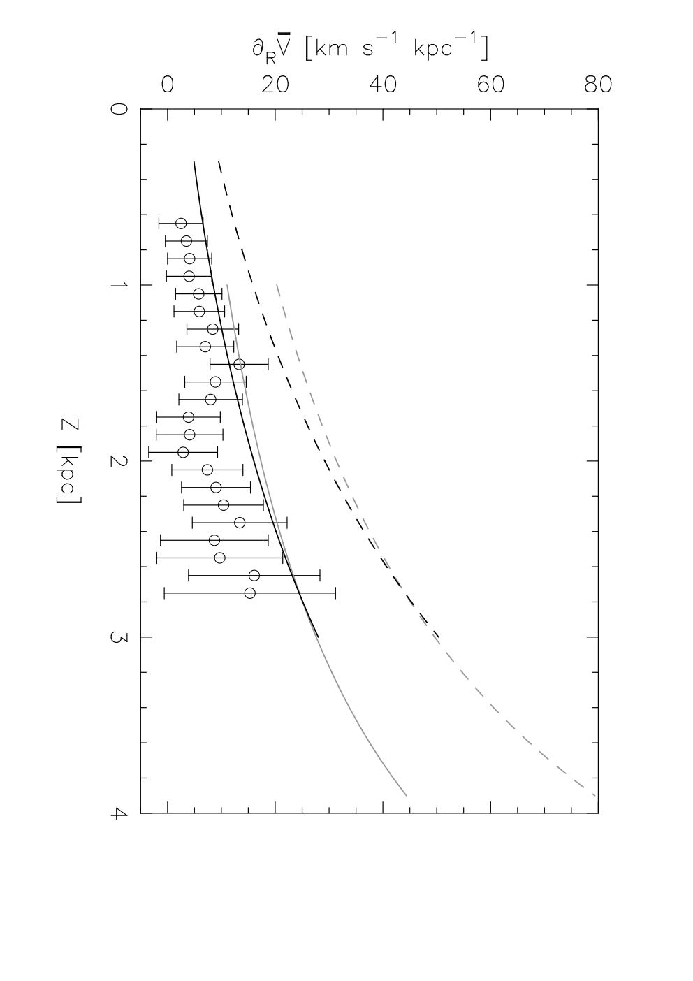
We collected from the Sloan Digital Sky Survey (York et al., 2000, SDSS,) DR7 database22 2 http://www.sdss3.org/ the photometric and spectroscopic data of stars with 20.2, 0.480.55, S/N15, 4.2, 0.25[/Fe]0.3, [Fe/H], and error on metallicity and -elements abundance lower than 0.25 dex. These criteria were adopted to select old, intermediate-metallicity G-type dwarf stars, as discussed in Carrell et al. (2012) and Bovy et al. (2012b). Their distance was estimated photometrically as in Ivezić et al. (2008). The Galactic coordinates, radial velocity, proper motion, and distance of each star were then transformed into () cylindrical coordinates and the respective () spatial velocities, and the errors on the former quantities were propagated to derive the final uncertainties. Only the 1096 stars with =7–9 kpc were considered in the analysis.
The azimuthal velocity of the resulting sample decreases with by km s-1 kpc-1, as shown in Fig. 4. This vertical shear is identical to what is found by 25 (see 25 for a comparison with previous studies). The rotational properties of the two samples are therefore very similar, indicating that they probe the same Galactic stellar population. The SDSS sample can therefore be used to study for the test population studied by 26 and 3.
We fitted a linear relation to in bins of width 0.5 kpc in steps of =0.1 kpc. A 2- clipping algorithm was adopted to remove outliers, which are mainly residual halo contaminators and bad measurements. The mean azimuthal velocity of these stars is constant with in both cases. As a consequence, decreased at all heights if this clipping was not applied, while the results were stable if the cut was stronger. The results are plotted in Fig. 5, where they are compared to the expectations of the 3 assumption. The quantity increases slowly from 5 km s-1 kpc-1 at =1 kpc to 13 km s-1 kpc-1 at =2.5–3 kpc. This trend matches the results of 5 extremely well. The SDSS data thus confirm all the conclusions drawn in Sect. 2.2.1 and, in particular, confirm that the 3 hypothesis largely overestimates at any heights.
2.2.3 Comparison with simulations

3 claim that the 26 hypothesis =0 is inconsistent with a flat radial profile of , while the steep increase in with discussed in Sect. 2.2 is its natural consequence. We tested this claim by means of orbit integration of a synthetic sample of stars. We adopted the Galactic potential model of Flynn et al. (1996), where the disk is represented by the sum of three MN disks and the dark halo by a spherical logarithmic potential. The contribution of the Galactic bulge and stellar halo are also included. The radial profile of in this model Galaxy is flat outside the solar circle. The test particles were spatially distributed as a double exponential disk with =0.9 kpc and =3.5 kpc. Their initial kinematics was fixed to match the trends of , , , and observed by 25 with the condition and an exponential radial decay of the dispersions with scale length =3.5 kpc. The system was then left to relax in the potential, and it rapidly achieved its steady state within the first Gyr of integration, although the experiment was stopped only after 5 Gyr. We then divided the sample in non-overlapping bins of 1000 stars with increasing , and we measured in each bin fitting the function
| (10) |
where , , and are the fit parameters. This functional form of the radial profile was chosen to account for the deviations from linearity at lower , as discussed in Sect. 2.2.1. An example of these fits is shown in Fig. 6 for the 1000 stars with =2.0–2.1 kpc.
The results of our experiment are shown in Fig. 7. We first imposed at any as the initial condition, and slightly increased during the integration. The system relaxed to tiny non-zero values with 5 km s-1 kpc-1 up to =4 kpc. This result indicates that the 26 hypothesis is wrong in this specific Galactic model, because a flat radial gradient of is not an equilibrium solution. In the second run, we imposed as initial condition the lowest 3 expectation, obtained from Equation (8) assuming the 26 parameters and the kinematical data of 5 (Figures 3, 5, and 7). Very surprisingly, the system relaxed to a profile identical to the first run, indicating that this is the real equilibrium configuration regardless of the initial conditions. This solution is much lower than the curves expected by the hypothesis, whose steep profile is therefore unstable in this Galactic potential model. This test demonstrates that low values of are consistent with a Milky Way-like galaxy, where =0 at the solar position, and a thick disk-like kinematics. The steep profile implied by the 3 formulation is therefore not a natural consequence of a radially constant circular velocity. It must be noted, however, that this counterexample alone does not prove that must be small for any Galactic potential model and initial conditions.

2.2.4 The validity of the assumption
We have shown that the observations, both in the Milky Way and in external galaxies, rule out the very peculiar thick disk kinematics required by the hypothesis , which is at the basis of the 3 formulation. Experiments of orbit integrations indicate that it is not a requirement of a flat radial profile of , and it is even an unstable configuration in the Milky Way-like potential adopted in the simulations.
The failure of the underlying assumption necessarily flaws the results of 3. It also invalidates the claim that their estimate is a lower limit to accurate within 20%. All evidence points to , because is much lower than the values required to have . 3 thus overestimate the mass density, because they neglect a negative contribution in Equation (3) or, equivalently, because they implicitly assume values of that are too high (see Figures 3, 5, and 7), whose integral gives a positive contribution to (see Equation (11)). This bias is severe for their preferred solution (Figures 3, 5, and 7), which yields mM⊙ pc-3. However, this overestimate is present even when assuming =0.9 kpc and =3.8 kpc, and the corresponding 3 solution for (compatible with mM⊙ pc-3) must also be biased.
3 Moni Bidin et al. (2012) revisited
The results presented in Sect. 2.2 evidence that the 26 hypothesis is only a rough approximation, and a more precise estimate of the mass density can be derived if it is dropped. In this case, the 26 expression becomes
| (11) |
where
| (12) |
The quantity cannot be estimated from 25 data, but the 5 results can be used. In fact, the two data sets probe the same stellar population (the intermediate-metallicity thick disk), as demonstrated by the fact that their kinematical results are fully compatible. A small mismatch in the mean metallicity would only have tiny effects on the kinematics (Bovy et al., 2012a). In any case, our aim here is not a complete revision of the 26 results, but to check to what extent these are biased by the assumption .
The studies of the Galactic disk measure the kinematical quantities only beyond a minimum Galactic height , because many observational limitations prevent us from tracking their trend down to the Galactic plane. The estimate of thus requires the extrapolation of the kinematics for . Calculating the surface density of the mass enclosed between and ,
| (13) |
is more appropriate in this case. 26 argue that their estimate of is not biased by the extension of the integration to lower , and they obtained identical results analyzing both and . Nevertheless, the general reliability of this extrapolation is not proven, and it is even less safe for Equation (11), which includes the previously neglected quantity . We therefore do not extend the calculation beyond the interval where we have information about it, and we study up to =2.5 kpc. 3 also gave more importance to the increment of above than to its absolute value. Subtracting the expected visible mass from the result, as defined by 26, we derive the mean DM density in the range =1–2.5 kpc, (1–2.5 kpc). It must be noted that the DM density derived from is nearly insensitive to the assumed visible mass model when kpc, because most of it lies below the volume under analysis. In fact, had different estimates from the literature been assumed (Holmberg & Flynn, 2000; Garbari et al., 2011, e.g.,), the (1–2.5 kpc) would vary by less than 0.2 mM⊙ pc-3.

Our results are shown in Fig. 8, overplotted to a set of curves of constant DM density. We first estimated by fitting the three measurements of 5 shown in Fig. 3. By inserting the result in Equation (11) along with the other kinematical quantities from 25 and the thick disk parameters preferred by 3 (=2.0 kpc, =3.5 kpc, and =0.7 kpc), the curve of returns mM⊙ pc-3. A higher DM density ( mM⊙ pc-3) can be recovered assuming the geometrical parameters =3.6 kpc and =0.9 kpc from the extensive survey of Jurić et al. (2008). Nevertheless, these results are only upper limits because, as discussed in Section 2.2.1, 5 probably overestimate . If the expression for is derived from the revised values of presented in Section 2.2.1 (Fig. 3), we obtain mM⊙ pc-3 when using the 3 geometrical parameters, and mM⊙ pc-3 when adopting the values from Jurić et al. (2008).
Similar results are found when , and are taken from 5, and we obtain mM⊙ pc-3, with an upper limit of mM⊙ pc-3. These estimates are consistent with those obtained above, but they are poorly informative because of the large errors.
4 Discussion and conclusions
We have shown that the validity of the 3 hypothesis depends on the underlying mass distribution. This means that they implicitly constrain the mass distribution to measure the mass density in a given volume. Even the validity of their claim that their estimate is a lower limit to accurate within 20% depends on these constraints.
The assumption predicts a very peculiar behavior for the Galactic thick disk rotation, ruled out by the observations of both the Milky Way and external galaxies. The results of 3 are flawed by this hypothesis. More specifically, they overestimate the mass density, because their formulation implicitly assumes values of that are too large (see Equation (11)). The observations also indicate that the 26 assumption is only a rough approximation, but we find that it does not bias the results noticeably. In fact, when this assumption is dropped and is taken from literature measurements, the resulting mean DM density at the solar position between =1 and 2.5 kpc is mM⊙ pc-3, with an upper limit of mM⊙ pc-3. The thick disk parameters preferred by 3 return much lower values. These results agree well with those of 26, demonstrating that the incidence of on the calculation is small. The resulting lack of DM is therefore not a systematic effect introduced by the aforementioned assumption. More investigation is needed to understand the peculiar results found by 26.
The uncertainties quoted here and in 26 result from rigorous propagation of errors on the input quantities, and they represent the statistical uncertainties well. Possible systematic errors are not considered in the error budget, but 26 analyzed most of their hypotheses and found no relevant bias. Their uncertainties are small when compared to the literature, but it must be considered that their calculation is extended in a volume that is four times larger than before. In fact, the extrapolation of the expected small DM contribution in the first kpc from the Galactic plane (25% of the total mass) is necessarily more uncertain than its estimate in a volume where it exceeds the quantity of visible mass. For example, a 10% uncertainty on the total mass and on the visible component propagates to a 40% error on at kpc, but this reduces to 20% and 10% at 4 kpc, respectively. The volume analyzed here is smaller than 26, and the resulting errors are larger by a factor of three. Our uncertainties are also partially enhanced by , an additional source of error not constrained very well by the data. As a result, our final errors are 30% larger than those quoted by Zhang et al. (2013), although our volume is comparable to theirs.
The results presented here are at variance with the expectations of a classical spherical DM halo with mM⊙ pc-3, whose density decreases by only 5% between =0 and 2 kpc. A deeper comprehension of the power and limitations of the 26 three-dimensional approach is required to fully understand this discrepancy. We nevertheless note that, while a low density on the plane is compatible only with a highly prolate halo (26, see), a low mean density in the range =1–2.5 kpc is compatible even with a very flat (oblate) distribution, if the bulk of the dark mass is found at kpc. It is also important to point out that the results obtained here are not directly comparable to previous estimates, because all similar measurements in the literature are limited to kpc.
All the literature measurements of the mass density at the solar position have adopted a one-dimensional approach, where the Galactic potential was modeled to match the observational data (but see Korchagin et al., 2003, for an exception). Both 3 and 26 make use of a direct equation, which relates the mass density to the kinematical quantities. 3 used the same kinematical data as 26, and share most of the assumptions with them but, after reducing the three-dimensional formulation of 26 to a one-dimensional approximation, found results in agreement with both classical works (Kuijken & Gilmore, 1989; Holmberg & Flynn, 2000, e.g.) and more recent studies (Siebert et al., 2003; Zhang et al., 2013, e.g.). Thus, they eventually prove that the discrepancy between the 26 results and the literature is most likely due neither to their use of a direct equation nor to a bias in the kinematical measurements. Their unexpected results most likely stem from their innovative three-dimensional approach, and more investigation is needed to understand them.
Acknowledgements.
R.A.M. acknowledges support from the Chilean Centro de Excelencia en Astrofísica y Tecnologías Afines (CATA) BASAL PFB/06, and by Project IC120009 “Millennium Institute of Astrophysics (MAS)” of the Iniciativa Científica Milenio del Ministerio de Economía, Fomento y Turismo de Chile. R.S. was financed by FONDECYT grant 3120135. Funding for SDSS-III has been provided by the Alfred P. Sloan Foundation, the Participating Institutions, the National Science Foundation, and the U.S. Department of Energy Office of Science. R.A.M. acknowledges ESO/Chile for hosting him during his sabbatical leave.References
- Bovy et al. (2012a) Bovy, J., Rix, H.-W., Hogg, D. W., et al. 2012a, ApJ, 755, 115
- Bovy et al. (2012b) Bovy, J., Rix, H.-W., Liu, C., et al. 2012b, ApJ, 753, 148
- Bovy & Tremaine (2012) Bovy, J. & Tremaine, S. 2012, ApJ, 756, 89
- Carrell et al. (2012) Carrell, K., Chen, Y., & Zhao, G. 2012, AJ, 144, 185
- Casetti-Dinescu et al. (2011) Casetti-Dinescu, D. I., Girard, T. M., Korchagin, V. I., & van Altena, W. F. 2011, ApJ, 728, 7
- Chiba & Beers (2000) Chiba, M. & Beers, T. C. 2000, AJ, 119, 2843
- Creze et al. (1998) Creze, M., Chereul, E., Bienayme, O., & Pichon, C. 1998, A&A, 329, 920
- Einasto (1965) Einasto, J. 1965, Trudy Astrofizicheskogo Instituta Alma-Ata, 5, 87
- Einasto (1968) Einasto, J. 1968, Publications of the Tartu Astrofizica Observatory, 36, 414
- Flynn et al. (1996) Flynn, C., Sommer-Larsen, J., & Christensen, P. R. 1996, MNRAS, 281, 1027
- Garbari et al. (2012) Garbari, S., Liu, C., Read, J. I., & Lake, G. 2012, MNRAS, 425, 1445
- Garbari et al. (2011) Garbari, S., Read, J. I., & Lake, G. 2011, MNRAS, 416, 2318
- Girard et al. (2006) Girard, T. M., Korchagin, V. I., Casetti-Dinescu, D. I., et al. 2006, AJ, 132, 1768
- Holmberg & Flynn (2000) Holmberg, J. & Flynn, C. 2000, MNRAS, 313, 209
- Ivezić et al. (2008) Ivezić, Ž., Sesar, B., Jurić, M., et al. 2008, ApJ, 684, 287
- Jałocha et al. (2010) Jałocha, J., Bratek, Ł., Kutschera, M., & Skindzier, P. 2010, MNRAS, 407, 1689
- Jurić et al. (2008) Jurić, M., Ivezić, Ž., Brooks, A., et al. 2008, ApJ, 673, 864
- Kalberla (2003) Kalberla, P. M. W. 2003, ApJ, 588, 805
- Kerr & Lynden-Bell (1986) Kerr, F. J. & Lynden-Bell, D. 1986, MNRAS, 221, 1023
- Korchagin et al. (2003) Korchagin, V. I., Girard, T. M., Borkova, T. V., Dinescu, D. I., & van Altena, W. F. 2003, AJ, 126, 2896
- Kregel et al. (2004) Kregel, M., van der Kruit, P. C., & Freeman, K. C. 2004, MNRAS, 351, 1247
- Kuijken & Gilmore (1989) Kuijken, K. & Gilmore, G. 1989, MNRAS, 239, 605
- Majewski (1992) Majewski, S. R. 1992, ApJS, 78, 87
- Miyamoto & Nagai (1975) Miyamoto, M. & Nagai, R. 1975, PASJ, 27, 533
- Moni Bidin et al. (2012a) Moni Bidin, C., Carraro, G., & Méndez, R. A. 2012a, ApJ, 747, 101
- Moni Bidin et al. (2012b) Moni Bidin, C., Carraro, G., Méndez, R. A., & Smith, R. 2012b, ApJ, 751, 30
- Moni Bidin et al. (2010) Moni Bidin, C., Carraro, G., Méndez, R. A., & van Altena, W. F. 2010, ApJ, 724, L122
- Navarro et al. (1997) Navarro, J. F., Frenk, C. S., & White, S. D. M. 1997, ApJ, 490, 493
- Olling (1995) Olling, R. P. 1995, AJ, 110, 591
- Olling & Merrifield (2001) Olling, R. P. & Merrifield, M. R. 2001, MNRAS, 326, 164
- Purcell et al. (2009) Purcell, C. W., Bullock, J. S., & Kaplinghat, M. 2009, ApJ, 703, 2275
- Qu et al. (2011) Qu, Y., Di Matteo, P., Lehnert, M. D., & van Driel, W. 2011, A&A, 530, A10
- Read et al. (2008) Read, J. I., Lake, G., Agertz, O., & Debattista, V. P. 2008, MNRAS, 389, 1041
- Reid et al. (1999) Reid, M. J., Readhead, A. C. S., Vermeulen, R. C., & Treuhaft, R. N. 1999, ApJ, 524, 816
- Salucci et al. (2010) Salucci, P., Nesti, F., Gentile, G., & Frigerio Martins, C. 2010, A&A, 523, A83
- Sanders (2012) Sanders, J. 2012, MNRAS, 425, 2228
- Siebert et al. (2003) Siebert, A., Bienaymé, O., & Soubiran, C. 2003, A&A, 399, 531
- Sofue et al. (2009) Sofue, Y., Honma, M., & Omodaka, T. 2009, PASJ, 61, 227
- Weber & de Boer (2010) Weber, M. & de Boer, W. 2010, A&A, 509, A25
- Yoachim & Dalcanton (2005) Yoachim, P. & Dalcanton, J. J. 2005, ApJ, 624, 701
- Yoachim & Dalcanton (2008) Yoachim, P. & Dalcanton, J. J. 2008, ApJ, 682, 1004
- York et al. (2000) York, D. G., Adelman, J., Anderson, Jr., J. E., et al. 2000, AJ, 120, 1579
- Zhang et al. (2013) Zhang, L., Rix, H.-W., van de Ven, G., et al. 2013, ApJ, 772, 108