Venmugil Elango The Ohio State University elango.4@osu.edu \authorinfoFabrice Rastello Inria Fabrice.Rastello@inria.fr \authorinfoLouis-Noël Pouchet The Ohio State University pouchet@cse.ohio-state.edu \authorinfoJ. Ramanujam Louisiana State University ram@cct.lsu.edu \authorinfoP. Sadayappan The Ohio State University saday@cse.ohio-state.edu
On Characterizing the Data Access Complexity of Programs
Abstract
Technology trends will cause data movement to account for the majority of energy expenditure and execution time on emerging computers. Therefore, computational complexity will no longer be a sufficient metric for comparing algorithms, and a fundamental characterization of data access complexity will be increasingly important. The problem of developing lower bounds for data access complexity has been modeled using the formalism of Hong & Kung’s red/blue pebble game for computational directed acyclic graphs (CDAGs). However, previously developed approaches to lower bounds analysis for the red/blue pebble game are very limited in effectiveness when applied to CDAGs of real programs, with computations comprised of multiple sub-computations with differing DAG structure. We address this problem by developing an approach for effectively composing lower bounds based on graph decomposition. We also develop a static analysis algorithm to derive the asymptotic data-access lower bounds of programs, as a function of the problem size and cache size.
Keywords:
Acategory
F.2 Analysis of Algorithms and Problem Complexity Generalcategory
D.2.8 Software Metricskeywords
Complexity measureskeywords
Data access complexity; I/O lower bounds; Red-blue pebble game; Static analysislgorithms, Theory
1 Introduction
Advances in technology over the last few decades have yielded significantly different rates of improvement in the computational performance of processors relative to the speed of memory access. Because of the significant mismatch between computational latency and throughput when compared to main memory latency and bandwidth, the use of hierarchical memory systems and the exploitation of significant data reuse in the faster (i.e., higher) levels of the memory hierarchy is critical for high performance. With future systems, the cost of data movement through the memory hierarchy is expected to become even more dominant relative to the cost of performing arithmetic operations Bergman et al. [2008]; Fuller and Millett [2011]; Shalf et al. [2011], both in terms of time and energy. It is therefore of critical importance to limit the volume of data movement to/from memory by enhancing data reuse in registers and higher levels of the cache. Thus the characterization of the inherent data access complexity of computations is extremely important.
⬇ for(i=1;i<N-1;i++) for(j=1;j<N-1;j++) A[i,j]=A[i-1,j]+A[i,j-1];
⬇ for(it=1;it<N-1;it+=T) for(jt=1;jt<N-1;jt+=T) for(i=it;i<min(it+T,N-1);i++) for(j=jt;j<min(jt+T,N-1);j++) A[i,j]=A[i-1,j]+A[i,j-1];

Let us consider the code shown in Fig. 1(a). Its computational complexity can be simply stated as arithmetic operations. Fig. 1(b) shows a functionally equivalent form of the same computation, after a tiling transformation. The tiled form too has exactly the same computational complexity of arithmetic operations. Next, let us consider the data access cost for execution of these two code forms on a processor with a single level of cache. If the problem size is larger than cache capacity, the number of cache misses would be higher for the untiled version (Fig. 1(a)) than the tiled version (Fig. 1(b)). But if the cache size were sufficiently large, the tiled version would not offer any benefits in reducing cache misses.
Thus, unlike the computational complexity of an algorithm, which stays unchanged for different valid orders of execution of its operations and also independent of machine parameters like cache size, the data access cost depends both on the cache capacity and the order of execution of the operations of the algorithm.
A fundamental question therefore is: Given a computation and the amount of storage at different levels of the cache/memory hierarchy, what is the minimum possible number of data transfers at the different levels, among all valid schedules that perform the operations?
In order to model the range of valid scheduling orders for the operations of an algorithm, it is common to use the abstraction of the computational directed acyclic graph (CDAG), with a vertex for each instance of each computational operation, and edges from producer instances to consumer instances. Fig. 1(c) shows the CDAG for the codes in Fig. 1(a) and Fig. 1(b), for =6; although the relative order of operations is different between the tiled and untiled versions, the set of computation instances and the producer-consumer relationships for the flow of data are exactly the same (special “input” vertices in the CDAG represent values of elements of that are read before they are written in the nested loop).
While in general it is intractable to precisely answer the above fundamental question on the absolute minimum number of data transfers between main memory and caches/registers among all valid execution schedules of a CDAG, it is feasible to develop lower bounds on the optimal number of data transfers.
An approach to developing a lower bound on the minimal data movement for a computation in a two-level memory hierarchy was addressed in the seminal work of Hong & Kung by using the model of the red/blue pebble game on a computational directed acyclic graph (CDAG) Hong and Kung [1981]. While the approach has been used to develop I/O lower bounds for a small number of homogeneous computational kernels, as elaborated later, it poses challenges for effective analysis of full applications that are comprised of a number of parts with differing CDAG structure.
In this paper, we address the problem of analysis of affine loop programs to develop lower bounds on their data movement complexity. The work presented in this paper makes the following contributions:
- •
Enabling composition in analysis of data access lower bounds: It adapts the Hong & Kung pebble game model on CDAGs and the associated model of S-partitioning under a restriction that disallows recomputation, thereby enabling effective composition of I/O lower bounds for composite CDAGs from lower bounds for component CDAGs.
- •
Static analysis of programs for lower bounds characterization: It develops an approach for asymptotic parametric analysis of data-access lower bounds for arbitrary affine loop programs, as a function of cache size and problem size. This is done by analyzing linearly independent families of non-intersecting dependence chains.
2 Background
2.1 Computational Model
We are interested in modeling the inherent data access complexity of a computation, defined as the minimum number of data elements to be moved between local memory (with limited capacity but fast access by the processor) and main memory (much slower access but unlimited capacity) among all valid execution orders for the operations making up the computation. While the key developments in this paper can be naturally extended to address multi-level memory hierarchies and parallel execution, using an approach like the MMHG (Multiprocessor Memory Hierarchy Game) model of Savage & Zubair Savage and Zubair [2008], we restrict the treatment in this paper to the case of only two levels of memory hierarchy and sequential execution.
The model of computation we use is a computational directed acyclic graph (CDAG), where computational operations are represented as graph vertices and the flow of values between operations is captured by graph edges. Fig. 2 shows an example of a CDAG corresponding to a simple loop program. Two important characteristics of this abstract form of representing a computation are that (1) there is no specification of a particular order of execution of the operations: although the program executes the operations in a specific sequential order, the CDAG abstracts the schedule of operations by only specifying partial ordering constraints as edges in the graph; (2) there is no association of memory locations with the source operands or result of any operation. (labels in Fig. 2 are only shown for aiding explanation; they are not part of the formal description of a CDAG).
for (i = 1; i < 4; ++i)
  S += A[i-1] + A[i];

We use the notation of Bilardi & Peserico Bilardi and Peserico [2001] to formally describe the CDAG model used by Hong & Kung:
Definition 1 (CDAG-HK)
A computational directed acyclic graph (CDAG) is a 4-tuple of finite sets such that: (1) is the input set and all its vertices have no incoming edges; (2) is the set of edges; (3) is a directed acyclic graph; (4) is called the operation set and all its vertices have one or more incoming edges; (5) is called the output set.

2.2 The Red-Blue Pebble Game
Hong & Kung used this computational model in their seminal work Hong and Kung [1981]. The inherent I/O complexity of a CDAG is the minimal number of I/O operations needed while optimally playing the Red-Blue pebble game. This game uses two kinds of pebbles: a fixed number of red pebbles that represent the small fast local memory (could represent cache, registers, etc.), and an arbitrarily large number of blue pebbles that represent the large slow main memory.
Definition 2 (Red-Blue pebble game Hong and Kung [1981])
Let be a CDAG such that any vertex with no incoming (resp. outgoing) edge is an element of (resp. ). Given S red pebbles and an arbitrary number of blue pebbles, with an initial blue pebble on each input vertex, a complete calculation is any sequence of steps using the following rules that results in a final configuration with blue pebbles on all output vertices:
- R1 (Input)
-
A red pebble may be placed on any vertex that has a blue pebble (load from slow to fast memory),
- R2 (Output)
-
A blue pebble may be placed on any vertex that has a red pebble (store from fast to slow memory),
- R3 (Compute)
-
If all immediate predecessors of a vertex have red pebbles, a red pebble may be placed on (or moved to) 11 1 The original red-blue pebble game in Hong and Kung [1981] does not allow moving/sliding a red pebble from a predecessor vertex to a successor; we chose to allow it since it reflects real instruction set architectures. Others Savage [1995] have also considered a similar modification. But all our proofs hold for both the variants. (execution or “firing” of operation),
- R4 (Delete)
-
A red pebble may be removed from any vertex (reuse storage).
The number of I/O operations for any complete calculation is the total number of moves using rules R1 or R2, i.e., the total number of data movements between the fast and slow memories. The inherent I/O complexity of a CDAG is the smallest number of such I/O operations that can be achieved, among all complete calculations for that CDAG. An optimal calculation is a complete calculation achieving the minimum number of I/O operations.
Fig. 3 shows an example schedule for the CDAG in Fig. 2. Given S red pebbles and unlimited blue pebbles, goal of the game is to begin with blue pebbles on all input vertices, and finish with blue pebbles on all output vertices by following the rules in Definition 2 without using more than S red pebbles. Considering the case with three red pebbles (), one possible complete calculation for the CDAG in Fig. 3 is: {, , , , , , , , , , , , , , , , , , , }. The I/O cost of this complete calculation is 6 (which corresponds to the number of moves using rules and ). A different complete calculation for the same CDAG with I/O cost of 12 is given by: {, , , , , , , , , , , , , , , , , , , , , , , }. The I/O complexity of the CDAG is the minimum I/O cost of all such complete calculations.
2.3 Lower Bounds on I/O Complexity via S-Partitioning
While the red-blue pebble game provides an operational definition for the I/O complexity problem, it is generally not feasible to determine an optimal calculation on a CDAG. Hong & Kung developed a novel approach for deriving I/O lower bounds for CDAGs by relating the red-blue pebble game to a graph partitioning problem defined as follows.
Definition 3 (Hong & Kung S-partitioning of a CDAG Hong and Kung [1981])
Let be a CDAG. An S-partitioning of C is a collection of subsets of such that:
- P1
-
, and
- P2
-
there is no cyclic dependence between subsets
- P3
-
- P4
-
where a dominator set of , is a set of vertices such that any path from to a vertex in contains some vertex in ; the minimum set of , is the set of vertices in that have all its successors outside of ; and for a set A, is the cardinality of the set A.
Hong & Kung showed a construction for a 2S-partition of a CDAG, corresponding to any complete calculation on that CDAG using S red pebbles, with a tight relationship between the number of vertex sets in the 2S-partition and the number of I/O moves in the complete calculation, as shown in Theorem 1. The tight association between any complete calculation and a corresponding 2S-partition provides the key Lemma 1 that serves as the basis for Hong & Kung’s approach for deriving lower bounds on the I/O complexity of CDAGs typically by reasoning on the maximal number of vertices that could belong to any vertex-set in a valid 2S-partition.
Theorem 1 (Pebble game, I/O and 2S-partition Hong and Kung [1981])
Any complete calculation of the red-blue pebble game on a CDAG using at most S red pebbles is associated with a 2S-partition of the CDAG such that where is the number of I/O moves in the complete calculation and is the number of subsets in the 2S-partition.
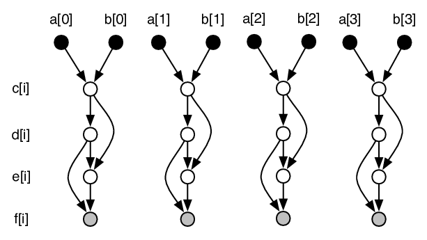
for(i = 0; i < 4; i++)
  c[i] = a[i] + b[i]; // S1
for(i = 0; i < 4; i++)
  d[i] = c[i] * c[i]; // S2
for(i = 0; i < 4; i++)
  e[i] = c[i] + d[i]; // S3
for(i = 0; i < 4; i++)
  f[i] = d[i] * e[i]; // S4
(a) Original code
(b) Full CDAG
(c) CDAG partitioning
Lemma 1 (Lower bound on I/O Hong and Kung [1981])
Let H be the minimal number of vertex sets for any valid -partition of a given CDAG (such that any vertex with no incoming – resp. outgoing – edge is an element of – resp. ). Then the minimal number Q of I/O operations for any complete calculation on the CDAG is bounded by:
This key lemma has been useful in proving I/O lower bounds for several CDAGs Hong and Kung [1981] by reasoning about the maximal number of vertices that could belong to any vertex-set in a valid 2S-partition.
3 Challenges in Composing I/O Lower Bounds from Partitioned CDAGs
Application codes are typically constructed from a number of sub-computations using the fundamental composition mechanisms of sequencing, iteration and recursion. As explained in Sec. 1, in contrast to analysis of computational complexity of such composite application codes, I/O complexity analysis poses challenges. With computational complexity, the operation counts of sub-computations can simply be added. However, using the red/blue pebble game model of Hong & Kung, as elaborated below, it is problematic to analyze the I/O complexity of sub-computations and simply combine them by addition. In the next section, we develop an approach to overcome the problem.
3.1 The Decomposition Problem
The Hong & Kung red/blue pebble game model places blue pebbles on all CDAG vertices without predecessors, since such vertices are considered to hold inputs to the computation, and therefore assumed to start off in slow memory. Similarly, all vertices without successors are considered to be outputs of the computation, and must have blue pebbles at the end of a complete calculation. If the vertices of a CDAG corresponding to a composite application are disjointly partitioned into sub-DAGs, the analysis of each sub-DAG will require the initial placement of blue pebbles on all vertices without predecessors in the sub-DAG, and final placement of blue pebbles on all vertices without successors in the sub-DAG. So an optimal calculation for each sub-DAG will require at least one load (R1) operation for each input and a store (R2) operation for each output. But in a complete calculation on the full composite CDAG, clearly it may be possible to pass values in a red pebble between vertices in different sub-DAGs, so that the I/O complexity could be less than the sum of the I/O costs for optimal calculations on each sub-DAG. This is illustrated by the following example.
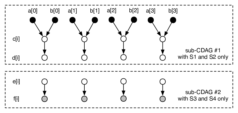
Fig. 4(b) shows the CDAG for the computation in Fig. 4(a). Fig. 4(c) shows the CDAG partitioned into two sub-DAGs, where the first sub-DAG contains vertices of and (and the input vertices corresponding to a[i] and b[i]), and the second sub-DAG contains vertices of and . Considering the full CDAG, with just two red pebbles, it can be computed at an I/O cost of , incurring I/O just for the initial loads of inputs a[i] and b[i], and the final stores for outputs f[i]. In contrast, with the partitioned sub-DAGs, the first sub-DAG will incur additional output stores for the successor-free vertices , and the second sub-DAG will incur input loads for predecessor-free vertices . Thus the sum of optimal red/blue pebble game I/O costs for the two sub-DAGs amounts to moves, i.e., it exceeds the optimal I/O cost for the full CDAG.
The above example illustrates a fundamental problem with the Hong & Kung red/blue pebble game model: a simple combining of I/O lower bounds for sub-DAGs of a CDAG cannot be used to generate an I/O lower bound for the composite CDAG. But the ability to perform complexity analysis by combining analyses of component sub-computations is important for the analysis of real applications. Such decomposition of data-access complexity analysis can be enabled by making a change to the Hong & Kung pebble game model, as discussed next.
3.2 Flexible Input/Output Vertex Labeling to Enable Composition of Lower Bounds
With the Hong & Kung model, all vertices without predecessors must be input vertices, and
all vertices without successors must be output vertices. By relaxing this
constraint, we show that composition of lower bounds from sub-CDAGs is
valid.
With such a modification,
vertices without predecessors will not be required to
be input vertices, and such predecessor-free non-input vertices
do not have an initial blue pebble
placed on them. However, such vertices are allowed to fire using
rule R3 at any time, since they do not have any predecessor nodes
without red pebbles. Vertices without successors
are similarly not required to be output vertices, and those not designated as
outputs do not need a blue pebble on them at the
end of the game. However, all compute vertices (i.e., vertices in
in CDAG are required
to have fired for any complete calculation.
Using the modified model of the red/blue pebble game with flexible input/output
vertex labeling, it is feasible to compose I/O lower bounds by adding
lower bounds for disjointly partitioned sub-CDAGs of a CDAG.
The following theorem formalizes it.
Theorem 2 (Decomposition)
Let be a CDAG. Let be an arbitrary (not necessarily acyclic) disjoint partitioning of ( and ) and be the induced partitioning of (, , ). If Q is the I/O complexity for and is the I/O complexity for , then . In particular, if is the I/O lower bound for , then is an I/O lower bound for .
Proof. Consider an optimal calculation for , with cost Q. We
define the cost of restricted to , denoted as , as the
number of or transitions in that involve a vertex of .
Clearly . We will show that we can build from , a valid
complete calculation for , of cost . This will prove that
, and thus . is built from
as follows: (1) for any transition in that involves a vertex
, apply this transition in ; (2) delete all other
transitions in . Conditions for transitions , , and are
trivially satisfied. Whenever a transition on a vertex is performed in
, all the predecessors of must have a red pebble on them. Since all
transitions of on the vertices of are maintained in , when is executed in , all its
predecessor vertices must have red pebbles, enabling transition .
With this modified model of the red/blue pebble game that permits predecessor-free vertices to be non-input vertices, complex CDAGs can be decomposed and lower bounds for the composite CDAG can be obtained by composition of the bounds from the sub-CDAGs. However, sub-CDAGs that have no “true” input and output vertices in them will have trivial I/O lower bounds of zero – the entire set of vertices in the sub-CDAG can fit in a single vertex set for a valid 2S-partition, for any value of S, since conditions P1-P4 are trivially satisfied.
In the next section, we present a solution to the problem. The main idea is to impose restrictions on the red/blue pebble game to disallow re-pebbling or multiple firings of any vertex using rule R3. We show that by imposing such a restriction, we can develop an input/output tagging strategy for sub-CDAGs that enables stronger lower bounds to be generated by CDAG decomposition.
4 S-Partitioning when Re-Pebbling is Prohibited
With the pebble game model of Hong & Kung, the compute rule R3 could be applied multiple times in a complete calculation. This is useful in modeling algorithms that perform re-computation of multiply used values rather than incur the overhead of storing and loading it. However, the majority of practically used algorithms do not perform any redundant recomputation. Hence several efforts Ballard et al. [2011]; Ballard et al. [2012b]; Bilardi and Peserico [2001]; Bilardi et al. [2012]; Scquizzato and Silvestri [2013]; Ranjan et al. [2011]; Savage [1995]; Savage [1998]; Savage and Zubair [2010]; Cook [1974]; Irony et al. [2004]; Ranjan et al. [2012]; Ranjan and Zubair [2012] have modeled I/O complexity under a more restrictive model that disallows recomputation, primarily because it eases or enables analysis with some lower bounding techniques. In this section, we consider the issue of composing bounds via CDAG decomposition under a model that disallows recomputation, i.e., prohibits re-pebbling. We develop a modified definition of S-partition that is adapted to enable I/O lower bounds to be developed for the restricted red/blue pebble game. This provides two significant benefits:
- 1.
It enables non-trivial I/O lower bound contributions to be accumulated from sub-CDAGs of a CDAG, even when the sub-CDAGs do not have any true inputs. This is achieved via input/output tagging/untagging strategies we develop in this section.
- 2.
It enables static analysis of programs to develop parametric expressions for asymptotic lower bounds as a function of cache and problem size parameters. This is described in the following sections.
A pebble game model that does not allow recomputation can be formalized by changing rule R3 of the red/blue pebble game to R3-NR (NR denotes No-Recomputation or No-Repebbling) and the definition of a complete calculation as follows:
Definition 4 (Recompute-restricted Red-Blue pebble game)
Let be a CDAG. Given S red pebbles and arbitrary number of blue pebbles, with an initial blue pebble on each input vertex, a complete calculation is any sequence of steps using the following rules that causes each vertex in to be fired once using Rule R3-NR, and results in a final configuration with blue pebbles on all output vertices:
- R1 (Input)
-
A red pebble may be placed on any vertex that has a blue pebble (load from slow to fast memory),
- R2 (Output)
-
A blue pebble may be placed on any vertex that has a red pebble (store from fast to slow memory),
- R3-NR (Compute)
-
If all immediate predecessors of a vertex have red pebbles on them, and a red pebble has not previously been placed on , a red pebble may be placed on .
- R4 (Delete)
-
A red pebble may be removed from any vertex (reuse storage).
We next present an adaptation of Hong and Kung’s S-partition that will enable us to develop larger lower bounds for the restricted pebble game model that prohibits repebbling.
Definition 5 (-partitioning of CDAG)
Given a CDAG C, an -partitioning of C is a collection of subsets of such that:
- P1
-
, and
- P2
-
there is no cyclic dependence between subsets
- P3
-
- P4
-
where the input set of , is the set of vertices of that have at least one successor in ; the output set of , is the set of vertices of that are also part of the output set or that have at least one successor outside of .
Theorem 3 (Restricted pebble game, I/O and -partition)
Any complete calculation of the red-blue pebble game, without repebbling, on a CDAG using at most S red pebbles is associated with a -partition of the CDAG such that where is the number of I/O moves in the game and is the number of subsets in the -partition.
Proof. Consider a complete calculation that corresponds to some scheduling (i.e., execution) of the vertices of the graph that follows the rules R1–R4 of the restricted pebble game. We view this calculation as a string that has recorded all the transitions (applications of pebble game rules). Suppose that contains exactly transitions of type or . Let correspond to a partitioning of the transitions of into consecutive sub-sequences such that each contains exactly S transitions of type or .
The CDAG contains no node isolated from the output nodes, and any vertex of is computed exactly once in . Let be the set of vertices computed (transition R3-NR) in the sub-calculation . Property is trivially fulfilled.
As transition R3-NR on a vertex is possible only if its predecessor vertices have red pebbles on them, those predecessors are necessarily executed in some , and are thus part of a , . This proves property .
To prove , for a given we consider two sets: is the set of vertices that had a red pebble on them just before the execution of ; is the set of vertices on which a red pebble is placed according to rule (input) during . We have, . Thus . As there only S red pebbles, . Also by construction of , . This proves that (property ).
Property is proved in a similar way: is the set of
vertices that have a red pebble on them just after the execution of
; is the set of vertices of on which a blue
pebble is placed during according to rule . We have that
. Thus . As there are only
S red pebbles, . Also by construction of
, . This proves that (property ).
Lemma 2 (I/O lower bound for restricted pebble game)
Let be the minimal number of vertex sets for any valid -partition of a given CDAG. Then the minimal number Q of I/O operations for any complete calculation on the CDAG, without any repebbling, is bounded by:
The above theorem and lemma establish the relationship between complete calculations of the restricted pebble game and 2S-NR partitions. The critical difference between the standard S-partition of Hong & Kung and the S-NR partition is the validity condition pertaining to incoming edges into a vertex set in the partition: for the former the size of dominator sets is constrained to be no more than S, while for the latter the number of external vertices with edges into the vertex set is constrained by S. When a CDAG is decomposed into sub-CDAGs, very often some of the sub-CDAGs get isolated from the CDAG’s input and output vertices. This will lead to trivial (i.e., zero) lower bounds for such component sub-CDAGs. For the restricted pebble game, below we develop an approach to obtain tighter lower bounds for component sub-CDAGs that have become isolated from inputs and outputs of the full CDAG. The key idea is to allow any vertex without predecessors (resp. successors) to simulate an input (resp. output) vertex by specially tagging it so, and then adjusting the obtained lower bound to account for a one-time access cost for loading (resp. storing) such a tagged input (resp. output). The vertices of a CDAG remain unchanged, but the labeling (tag) of some vertices as inputs/outputs in the CDAG is changed.
Theorem 4 (Input/Output (Un)Tagging – Restricted pebble game)
Let and be two CDAGs of the same DAG : , , where, and . If Q is the I/O complexity for and is the I/O complexity for then, Q can be bounded by as follows (tagging):
| (1) |
Reciprocally, can be bounded by Q as follows (untagging):
| (2) |
Proof. Consider an optimal calculation for , of cost Q. We will build a valid complete calculation for , of cost no more than . This will prove that . We build from as follows: (1) for any input vertex , the (only) transition involving in is replaced in by a transition ; (2) for any output vertex , the (only) transition involving in is complemented by an transition; (3) any other transition in is reported as is in .
Consider now an optimal calculation for , of cost .
We will build a valid complete calculation for , of cost no
more than .
This will prove that . We build from as
follows:
(1) for any input vertex , the first transition involving
in is replaced in by a transition followed by a
transition ; (2) any other transition in is reported as is in
.
We note that such a construction is only possible for the restricted pebble game where repebbling is disallowed. It enables tighter lower bounds to be developed via CDAG decomposition. In the next section, we use S-NR partitioning and the untagging theorem in developing a static analysis approach to characterizing data-access lower bounds of loop programs.
5 Parametric Lower Bounds via Static Analysis of Programs
In this section, we develop a static analysis approach to derive asymptotic parametric I/O lower bounds as a function of cache size and problem size, for affine computations. Affine computations can be modeled using (union of) convex sets of integer points, and (union of) relations between these sets. The motivation is twofold. First, there exists an important class of affine computations whose control and data flow can be modeled exactly at compile-time using only affine forms of the loop iterators surrounding the computation statements, and program parameters (constants whose values are unknown at compile-time). Many dense linear algebra computations, image processing algorithms, finite difference methods, etc., belong to this class of programs Girbal et al. [2006]. Second, there exist readily available tools to perform complex geometric operations on such sets and relations. We use the Integer Set Library (ISL) Verdoolaege [2010] for our analysis.
In Subsection 5.1, we provide a description of the program representation for affine programs. In Subsection 5.2, we detail the geometric reasoning that is the basis for the developed I/O lower bounds approach. Subsection 5.3 describes the I/O lower bound computation using examples.
5.1 Background and Program Representation
In the following, we use ISL terminology Verdoolaege [2010] and syntax to describe sets and relations. We now recall some key concepts to represent program features.
Iteration domain
A computation vertex in a CDAG represents a dynamic instance
of some operation in the input program. For example,
given a statement A[i] += B[i+1]
surrounded by one loop for(i = 0; i < n; ++i), the operation
+= will be executed times, and each such dynamic
instance of the statement corresponds to a vertex in the CDAG.
For affine programs, this set of dynamic instances can be compactly
represented as a (union of) -polyhedra, i.e., a set of
integer points bounded by affine inequalities intersected with
an affine integer lattice Gupta and Rajopadhye [2007]. Using ISL notation, the
iteration domain of statement , , is denoted:
[n]->{S1[i]:0<=i<n}. The left-hand side of ->,
[n] in the example, is the list of all parameters needed to define the
set. S1[i] models a set with one dimension ([i]) named
, and the set space is named S1. Presburger
formulae are used on the right-hand side of : to model the points
belonging to the set. In ISL, these sets are disjunctions of
conjunctions of Presburger formulae, thereby modeling unions of convex
and strided integer sets. The dimension of a set is denoted as
. in the example above. The cardinality of set is denoted
as . for the example. Standard operations on sets,
such as union, intersection, projection along certain
dimensions, are available. In addition, key operations for analysis, such as
building counting polynomials for the set (i.e., polynomials of the
program parameters that model how many integer points are contained in
a set; in our example) Barvinok [1994], and parametric
(integer) linear programming Feautrier [1988] are possible on such
sets. These operations are available in ISL.
We remark that although our analysis relies on integer sets and their associated operations, it is not limited to programs that can be exactly captured using such sets (e.g., purely affine programs). Since we are interested in computing lower bounds on I/O, an under-approximation of the statement domain and/or the set of dependences is acceptable, since an I/O lower bound for the approximated system is a valid lower bound for the actual system. For instance, if the iteration domain of a statement is not described exactly using Presburger formulae, we can under-approximate this set by taking the largest convex polyhedron . Such a polyhedron can be obtained, for instance, by first computing the convex hull and then shifting its faces until they are strictly included in . We also remark that such sets can be extracted from an arbitrary CDAG (again using approximations) by means of trace analysis, and especially trace compression techniques for vertices modeling the same computation Ketterlin and Clauss [2012].
Relations
In the graph of a CDAG , vertices are connected by producer-consumer edges capturing the data flow between operations. Similar to iteration domains, affine forms are used to model the relations between the points in two sets. Such relations capture which data is accessed by a dynamic instance of a statement, as in classical data-flow analysis. In the example above, elements of array B are read in statement , and the relation describing this access is: [n]->{S1[i] -> B[i+1] : 0<=i<n}. This relation models a single edge between each element of set and an element of set , described by the relationship . Several operations on relations, such as , which computes the domain (e.g., input set) of the relation ( [n] -> {[i] : 0<=i<n}), computing the image (e.g., range, or output set) of ( [n] -> {[i] : 1<=i<n+1}), the composition of two relations , their union , intersection , difference and the transitive closure of a relation, are available. All these operations are supported by ISL.
Relations can also be used to directly capture the connections between computation vertices. For instance, given two statements and with a producer-consumer relationship, the edges connecting each dynamic instance of and in a CDAG can be expressed using relations. For example, [n]->{S1[i,j] -> S2[i,j-1,k] : ...} models a relation between a 2D statement and a 3D statement. Each point in is connected to several points in along the -dimension.
We note that in a similar manner to iteration domains for vertices, relations can also be extracted from non-affine programs via convex under-approximation or from the CDAG via trace analysis. Again, care must be taken to always properly under-approximate the relations capturing data dependences: it is safe to ignore a dependence (it can only lead to under-approximation of the data flow and therefore the I/O requirement), and therefore we only consider must-dependences in our analysis framework.
5.2 Geometric Reasoning for I/O Lower Bounds by 2S-partitioning
Given a CDAG, Lemma 2 establishes a relation between a lower bound on its data movement complexity for execution with fast storage elements and the minimal possible number of vertex sets among all valid -partitions of the CDAG. The minimum possible number of vertex sets in a -partition is inversely related to the largest possible size of any vertex set for a valid -partition. A geometric reasoning based on the Loomis-Whitney inequality Loomis and Whitney [1949] and its generalization Bennett et al. [2010]; Valdimarsson [2010] has been used to establish I/O lower bounds for a number of linear algebra algorithms Irony et al. [2004]; Ballard et al. [2011]; Ballard et al. [2012a]; Christ et al. [2013]. A novel approach to determining I/O lower bounds for affine computations in perfectly nested loops has been recently developed Christ et al. [2013] using similar geometric reasoning. The approach developed in this paper is inspired by that work and also uses a similar geometric reasoning, but improves on the prior work in two significant ways:
- 1.
Generality: It can be applied to a broader class of computations, handling multiple statements and imperfectly nested loops.
- 2.
Tighter Bounds: For computations with loop-carried dependences that are not oriented perfectly along one of the iteration space dimensions, it provides tighter I/O lower bounds, as illustrated by the Jacobi example in the next section.
Before presenting the details of the static analysis for lower bounds characterization of affine computations, we use a simple example to illustrate the geometric approach based on the Loomis-Whitney inequality and its generalizations that have been used to develop I/O lower bounds for matrix-multiplication and other linear algebra computations. Consider the code exemplifying an N-body force calculation in Fig. 5(a). We have a 2D iteration space with points. The net force on each of particles from the other particles is computed using the function f(), which uses the mass and position of a pair of particles to compute the force between them. The total number of input data elements for the computation is . If , it will be necessary to bring in at least some of the input data elements more than once from slow to fast memory. A geometric reasoning for a lower bound on the amount of I/O to/from fast memory proceeds as follows. Consider an arbitrary vertex set from any valid -partition. Let the set of points P in the iteration space, illustrated by a cloud in Fig. 5(b), denote the vertex set. The projections of each of the points onto the two iteration space axes are shown. Let and respectively denote the number of distinct points on the and axes. represents the number of distinct elements of input arrays pos and mass that are accessed in the computation, for references pos(i) and mass(i). Similarly, corresponds to the number of distinct elements accessed via the references pos(j) and mass(j). For any vertex set from a valid -partition, the size of the input set cannot exceed . Hence and . For this 2D example, the Loomis-Whitney inequality asserts that the number of points in P cannot exceed . Combining the two inequalities, we can conclude that is an upper bound on the size of the vertex set. Thus, the minimum number of vertex sets in a valid 2S-partition, . By Lemma 2, a lower bound on I/O is , i.e., .
⬇ for(i=0;i<N;i++) for(j=0;j<N;j++) if (i <> j) force(i) += f(mass(i),mass(j),pos(i),pos(j));

More generally, for a -dimensional iteration space, given some bounds on the number of elements on some projections of P, a bound on can be derived using a powerful approach developed by Christ et al. Christ et al. [2013]. Christ et al. [Christ et al., 2013, Theorem 3.2] extended the discrete case of the Brascamp-Lieb inequality [Bennett et al., 2010, Theorem 2.4] to obtain these bounds. Since our goal here is to develop asymptotic parametric bounds, the extension of the continuous Brascamp-Lieb inequality, stated below (in the restricted case of orthogonal projections and using the Lebesgue measure for volumes), is sufficient for our analysis. We use the notation to denote that is a linear subspace of .
Theorem 5
Let
be an orthogonal projection for such that
where .
Then, for :
| (3) | |||
| (4) |
Since the linear transformations are orthogonal projections, the following Theorem enables us to limit the number of inequalities of Eq. (3) required for Theorem 5 to hold. Only one inequality per subspace , defined as the linear span of the canonical vector , is required ( represents the subspace spanned by the vector with a non-zero only in the coordinate):
Theorem 6
Let
be an orthogonal projection for such that
where .
Then, for
| (5) | |||
| (6) |
where,
The proof of Theorem 6 directly corresponds to the proof of [Christ et al., 2013, Theorem 6.6] and is omitted (see also [Bennett et al., 2010, Prop. 7.1]). It shows that if are such that , then the volume of any measurable set can be bounded by . In order to obtain as tight an asymptotic bound as possible, we seek such that is as small as possible. Since we have , this corresponds to finding such that is minimized, or equivalently, is minimized. In other words, has to be minimized. For this purpose, if , we solve:
| (7) |
We can instead solve the following dual problem, whose solution gives an indication of the shape of the optimal “cube.”
| (8) |
We use an illustrative example:
Consider the following three projections (we explain how the projection directions are obtained later in this section)
Let , and denote the three subspaces spanned by the canonical bases of . Consider, for example, the linear map . We have for any , for any , and for any . Thus, we obtain the constraint , or . Similarly, we obtain the remaining two constraints for the projections and .
This results in the following linear programming problem:
| (9) |
s.t.
Solving Eq. (9) provides the solution , i.e., . The solution corresponds to considering a cube of asymptotic dimensions and volume = as the largest vertex-set. This provides an I/O lower bound of , when the problem size is sufficiently large.
5.3 Automated I/O Lower Bound Computation
We present a static analysis algorithm for automated derivation of expressions for parametric asymptotic I/O lower bounds for programs. We use two illustrative examples to explain the various steps in the algorithm before providing detailed pseudo-code for the algorithm.
Illustrative example 1:
Consider the following example of Jacobi 1D stencil computation.

Fig. 6 shows the static data-flow graph
for Jacobi 1D. contains a vertex for
each statement in the code. The input array I is also explicitly
represented in by node (shaded in black
in Fig.
6).
Each vertex has an associated domain as shown below:
- •
[N]->{I[i]:0<=i<N} - •
[N]->{S1[i]:0<=i<N} - •
[T,N]->{S2[t,i]:1<=t<T and 1<=i<N-1} - •
[T,N]->{S3[t,i]:1<=t<T and 1<=i<N-1}
The edges represent the true (read-after-write) data dependences between the statements. Each edge has an associated affine dependence relation as shown below:
- •
Edge : This edge corresponds to the dependence due to copying the inputs
Ito arrayAat statement and has the following relation.[N]->{I[i]->S1[i]:0<=i<N} - •
Edges , and : The use of array elements
A[i-1], A[i]andA[i+1]at statement are captured by edges , and , respectively.[T,N]->{S1[i]->S2[1,i+1]:1<=i<N-2} [T,N]->{S1[i]->S2[1,i]:1<=i<N-1} [T,N]->{S1[i]->S2[1,i-1]:2<=i<N-1} - •
Edges and : Multiple uses of the boundary elements
I[0]andI[N-1]byA[t][1]andA[t][N-2], respectively, for1<=t<Tare represented by the following relations.[T,N]->{S1[0]->S2[t,1]:1<=t<T}[T,N]->{S1[N-1]->S2[t,N-2]:1<=t<T} - •
Edge : The use of array
Bin statementS3corresponds to edge with the following relation.[T,N]->{S2[t,i]->S3[t,i]:1<=t<T and 1<=i<N-1} - •
Edges , and : The uses of array
Ain statement from are represented by these edges with the following relations.[T,N]->{S3[t,i]->S2[t+1,i+1]:1<=t<T-1 and 1<=i<N-2} [T,N]->{S3[t,i]->S2[t+1,i]:1<=t<T-1 and 1<=i<N-1} [T,N]->{S3[t,i]->S2[t+1,i-1]:1<=t<T-1 and 2<=i<N-1}
Given a path with associated edge relations , the relation associated with can be computed by composing the relations of its edges, i.e., . For instance, the relation for the path in the example, obtained through the composition , is given by [T,N] -> {S2[t,i] -> S2[t+1,i+1]}. Further, the domain and image of a composition are restricted to the points for which the composition can apply, i.e., and . Hence, [T,N] -> {S2[t,i] : 1<=t<T-1 and 1<=i<N-2} and [T,N] -> {S2[t,i] : 2<=t<T and 2<=i<N-1}.
Two kinds of paths, namely, injective circuit and broadcast path, defined below, are of specific importance to the analysis.
Definition 6 (Injective edge and circuit)
An injective edge is an edge of a data-flow graph whose associated relation is both affine and injective, i.e., , where is an invertible matrix. An injective circuit is a circuit of a data-flow graph such that every edge is an injective edge.
Definition 7 (Broadcast edge and path)
A broadcast edge is an edge of a data-flow graph whose associated relation is affine and . A broadcast path is a path of a data-flow graph such that is a broadcast edge and are injective edges.
Injective circuits and broadcast paths in a data-flow graph essentially indicate multiple uses of same data, and therefore are good candidates for lower bound analysis. Hence only paths of these two kinds are considered in the analysis. The current example of Jacobi 1D computation illustrates the use of injective circuits to derive I/O lower bounds, while the use of broadcast paths for lower bound analysis is explained in another example that follows.
Injective circuits: In the Jacobi example, we have three circuits to vertex through . The relation for each circuit is computed by composing the relations of its edges as explained earlier. The relations, and the dependence vectors they represent, are listed below.
- •
Circuit :
[T,N] -> {S2[t,i]->S2[t+1,i+1] : 1<=t<T-1 and 1<=i<N-2} - •
Circuit :
[T,N] -> {S2[t,i]->S2[t+1,i] : 1<=t<T-1 and 1<=i<N-1} - •
Circuit :
[T,N] -> {S2[t,i]->S2[t+1,i-1] : 1<=t<T-1 and 2<=i<N-1}

Fig. 7 pictorially shows the domain and the relation as a -polyhedron for .
Definition 8 (Frontier)
The frontier, , of a relation , with domain , is the set of points with no incoming edges in the corresponding -polyhedron.
can be calculated using the set operation . The frontiers , and for the three relations, , and respectively, are listed below.
- •
[T,N]->{S2[1,i]:2<=i<N-2; S2[t,1]:1<=t<T-1} - •
[T,N]->{S2[1,i]:1<=i<N-1} - •
[T,N]->{S2[1,i]:2<=i<N-1; S2[t,N-2]:2<=t<T-1}
In Fig. 7, points of frontier are shown as red diamond shaped points. Due to the correspondence between a -polyhedron and a (sub-)CDAG (refer to Sec. 5.1), each point in a frontier represents a source vertex (i.e., vertex with no incoming edges) of the (sub-)CDAG. It could be seen that there are , disjoint paths (as a consequence of the injective property of the relations) in the sub-CDAG (corresponding to the instances of statements and ), each with a distinct source vertex that corresponds to a point in . These source vertices are tagged as inputs for the lower bounds analysis and their count, , is later subtracted from the final I/O lower bound using Theorem 4.
Let be a vertex-set of a valid -partition of . There are a set of points in the -polyhedron (e.g., the set of points inside the gray colored box in Fig. 7) corresponding to . The set of points outside with an edge to a point in corresponds to (e.g., points marked with yellow triangles in Fig. 7). Since there is no cyclic dependence between the vertex-sets of the 2S-partition and the paths are disjoint, by starting from the vertices of and tracing backwards along the paths in any , we should reach distinct source vertices. This process corresponds to projecting the set along each of the directions onto the frontier . Hence we have (here, denotes projecting along the direction ). The points of the frontier obtained by projection are shown as black squares (over red diamonds) in Fig. 7. We ensure that . This allows us to apply the geometric reasoning discussed in Sec. 5.2 to restrict the size of the set as shown below. Since , it is sufficient to consider any two linearly independent directions.
Theorem 6 applies only for projections along the orthogonal directions. In case projection vectors are non-orthogonal, a simple change of basis operation is used to transform the space to a new space where the projection directions are the canonical bases. In the example, if we consider vectors and as the projection directions in the original space, then the linear map will transform the -polyhedron to a new space where the projection directions are the canonical bases. In the example, after such transformation, the projection vectors are and , and hence we have the following two projections: ; . From Eq. 6, we obtain the following inequalities for the dual problem (refer (8)): ; .
In addition, we also need to include constraints for the degenerate cases where the problem size considered may be small relative to the cache size, S. Hence, we have the following additional constraints for the example: ; , or (after taking with base S), ; . Since , we have . Hence, we obtain the constraints and . Thus, we solve the following following parametric linear programming problem.
| (10) |
Solving Eq. (10) using PIP Feautrier [1988] provides the
following solution:
If then, , else, .
This specifies that when , , and hence (here, is subtracted from the lower bound to account for I/O tagging), otherwise, and .
In the example, since the vectors and are already orthonormal, the change of basis transformation that we performed earlier is unimodular. But, in general this need not be the case. Since we focus only on asymptotic parametric bounds, any constant multiplicative factors that arise due to the non-unimodular transformation are ignored.
Illustrative example 2:
The following example is composed of a scaled matrix-multiplication and a Gauss-Seidel computation within an outer iteration loop.
The decomposition theorem (Theorem 2) allows us to split this code into individual components, analyze each sub-program separately and obtain the I/O lower bounds for the whole program through simple summation of the individual bounds. Hence, given the CDAG of the above example, the analysis proceeds with the following steps:
- •
The CDAG and thus the underlying program is decomposed as follows: (1) Each iteration of the outer loop, with trip-count W, is split into sub-programs. (2) Each of this sub-program is further decomposed by separating the matmult (consisting of statements and ) and Seidel operations (consisting of statement ) into individual sub-programs.
- •
The vertices corresponding to the input arrays of the matmult and Seidel computations are tagged as inputs in their corresponding sub-CDAGs.
- •
The matmult (with sub-CDAG ) and the Seidel computation (with sub-CDAG ) are separately analyzed for their I/O lower bounds.
- •
The analysis of the Seidel computation is similar to the analysis of the Jacobi 1D computation detailed in the previous example. Hence, we skip the analysis and provide the following result: If and then, , else . where, is the I/O complexity for the Seidel computation.
Now, we consider the analysis of the scaled matmult. The data-flow graph, consists of six vertices: vertices , and correspond to the input arrays A, C and Temp, respectively; vertices , and correspond to the statements , and , respectively. The domain corresponding to each vertex (in the order and ) is listed below:
- •
[N]->{A[i,j]:0<=i<N and 0<=j<N}
- •
[N]->{C[i,j]:0<=i<N and 0<=j<N}
- •
[N]->{Temp[i,j]:0<=i<N and 0<=j<N}
- •
[N]->{S1[i,j,k]:0<=i<N and 0<=j<N and 0<=k<N}
- •
[N]->{S2[i,j]:0<=i<N and 0<=j<N}
- •
[N]->{S3[i,j]:0<=i<N and 0<=j<N}
The relations corresponding to various edges are listed below.
- •
[N] -> {A[i, j] ->
S1[i,j’,j] : 0<=i<N and 0<=j<N and 0<=j’<N} - •
[N] -> {A[i,j] ->
S1[i’,j,i] : 0<=i’<N and 0<=i<N and 0<=j<N} - •
[N] -> {C[i,j] -> S3[i,j] : 0<=i<N and 0<=j<N}
- •
[N] -> {Temp[i,j] -> S1[i,j,0] : 0<=i<N and 0<=j<N}
- •
[N] -> {S1[i,j,k] ->
S1[i,j,k+1] : 0<=i<N and 0<=j<N and 0<=k<N-1} - •
[N] -> {S1[i,j,N-1] -> S2[i,j] : 0<=i<N and 0<=j<N}
- •
[N] -> {S2[i,j] -> S3[i,j] : 0<=i<N and 0<=j<N}
Broadcast paths: The paths and are of type broadcast. As and are composed of a single edge, their relations, and respectively, are the same as their edge. Thus, and . We are specifically interested in the broadcast paths whose inverse-relations (e.g., ) can be expressed as affine maps. In our example, the two inverse-relations and can be expressed as affine maps as shown below:
Further, we have an injective circuit with , whose direction vector .
We next calculate the frontiers and of the relations , and , respectively, by taking the set-difference of their domain and image (e.g., ), where, ). The three frontiers are shown using the ISL notation below:
- •
[N] -> {A[i,j] : 0<=i<N and 0<=j<N}
- •
[N] -> {A[i,j] : 0<=i<N and 0<=j<N}
- •
[N] -> {S1[i,j,0] : 0<=i<N and 0<=j<N}
In the case an injective circuit (with associated relation, say, ), we chose the direction of projection to be the vector representing . Here, in case of a broadcast path (with associated relation, say, ), we choose the kernel of the matrix , , to be the projection direction. The intuition behind choosing this direction is that the kernel represents the plane of reuse, and hence, the set of points obtained by projecting a set along the kernel directions represents the . In general, the kernel can be of dimension higher than one (but has to be at least one due to the definition of a broadcast path). The kernels ( and ) of the inverse-relations of the paths and are: and , respectively.
By choosing , and as the projection directions, we obtain ; ; . This provides us the following inequalities: ; ; . Further, to handle the degenerated cases, we have the additional constraints that specify that the size of the projections onto the subspaces , and { should not exceed and the size of the projections onto the subspaces , and should not exceed . Hence, we obtain the following parametric linear programming problem.
| (13) |
Solving Eq. (13) using PIP Feautrier [1988] provides the
following solution:
If then, , else,
.
Hence, when , , otherwise, .
Finally, by applying Theorem 2, we obtain the I/O lower bound for the full program, when and are sufficiently large.
Putting it all together:
Algorithm 1 provides a pseudo-code for our algorithm. Because the number of possible paths in a graph is highly combinatorial, several choices are made to limit the overall practical complexity of the algorithm. First, only edges of interest, i.e., those that correspond to relations whose image is representative of the iteration domain, are kept. Second, paths are considered in the order of decreasing expected profitability. One criterion detailed here corresponds to favoring injective circuits over broadcast paths with one-dimensional kernel (to reduce the potential span), and then broadcast paths with decreasing kernel dimension (the higher the kernel, the more the reuse, the lower the constraint).
For a given vertex , once the directions associated with the set of paths chosen so far span the complete space of the domain of , no more paths are considered. The role of the function try() (on lines 20, 26 and 32 in Algorithm 1) amounts to finding a set of paths that are linearly independent, compatible (i.e., a base can be associated to them), and representative. The funtion try() is shown in Algorithm 3. The function best() (shown in Algorithm 2) selects a set of paths for a vertex and computes the associated complexity. The function solve() (shown in Algorithm 4) writes the linear program and returns the I/O lower bound (with cases) for a domain and a set of compatible subspaces.
Various operations used in the pseudo-code are detailed below.
- •
Given a relation , and return the domain and image of , respectively.
- •
For an edge , the operation provides its associated relation. If has acceptable number of disjunctions, then the edge can be split into multiple edges with count equal to the number of disjunctions, otherwise, a convex under-approximation can be done.
- •
For a given path with associated relations we can compute the associated relation for by composing the relations of its edges, i.e., computes . Note that the domain of the composition of two relations is restricted to the points for which the composition can apply, i.e. and .
- •
For a given domain , returns its dimension. If the cardinality of (i.e., number of points in ) is represented in terms of the program parameters, its dimension can be obtained by setting the values of the parameters to a fixed big value (say ), and computing , and rounding the result to the nearest integer. For example, if , setting , we get .
- •
If a relation is injective and can be expressed as an affine map of the form , then the operation computes , otherwise, returns .
- •
For a relation , if its inverse can be expressed as an affine relation , computes the kernel of the matrix (and returns otherwise).
- •
For a set of vectors , provides the linear subspace spanned by those vectors.
- •
For a set of linear subspaces , gives a set of linearly independent vectors such that for any , there exists s.t. . If such a set could not be computed, it returns .
- •
For a path , returns its set of vertices.
- •
Given an expression , the operation simplifies the expression by eliminating the lower order terms. For example, returns .
| - | is a subspace, |
|---|---|
| - | is a set of subspaces, |
| - | is a domain, |
| - | is a set of vertices} |
6 Related Work
Hong & Kung provided the first formalization of the I/O complexity problem for a two-level memory hierarchy using the red/blue pebble game on a CDAG and the equivalence to 2S-partitions of the CDAG. We perform an adaptation of Hong & Kung 2S-partitioning to constrain the size of the input set of each vertex set rather than a dominator set, which is suitable for bounding the minimum I/O for a CDAG with the restricted red/blue pebble game where repebbling is disallowed. This adaptation enables effective composition of lower bounds of sub-CDAGs to form I/O lower bounds for composite CDAGs. A similar adaptation has previously been used by modifying the red/blue pebble game through addition of a third kind of pebble Elango et al. [2014]; Elango et al. [2013]. The composition of lower bounds for sequences of linear algebra operations has previously been addressed by the work of Ballard et al. Ballard et al. [2011] by use of “imposed” reads and writes in between segments of operations, adding the lower bounds on data access for each of the segments, and subtracting the number of imposed reads and writes. Our use of tagged inputs and outputs in conjunction with application of the decomposition theorem bears similarities to the use of imposed reads and writes by Ballard et al., but is applicable to the more general model of CDAGs that model data dependences among operations.
In Bilardi and Preparata [1999] an approach is proposed to obtain e lower bound to the access complexity of a DAG in terms of space lower bounds that apply to disjoint components of the DAG, when recomputation is not allowed. In Bilardi et al. [2000], the approach is extended to the case when recomputation is allowed, by means of the notion of free-input space complexity.
Irony et al. Irony et al. [2004] used a geometric reasoning with the Loomis-Whitney inequality Loomis and Whitney [1949] to present an alternate proof to Hong and Kung’s Hong and Kung [1981] for I/O lower bounds on standard matrix multiplication. More recently, Demmel’s group at UC Berkeley has developed lower bounds as well as optimal algorithms for several linear algebra computations including QR and LU decomposition and the all-pairs shortest paths problem Ballard et al. [2011]; Ballard et al. [2012b]; Demmel et al. [2012]; Solomonik et al. [2013].
Extending the scope of the Hong & Kung model to more complex memory hierarchies has also been the subject of research. Savage provided an extension together with results for some classes of computations that were considered by Hong & Kung, providing optimal lower bounds for I/O with memory hierarchies Savage [1995]. Valiant proposed a hierarchical computational model Valiant [2011] that offers the possibility to reason in an arbitrarily complex parametrized memory hierarchy model. While we use a single-level memory model in this paper, the work can be extended in a straight forward manner to model multi-level memory hierarchies.
Unlike Hong & Kung’s original model, several models have been proposed that do not allow recomputation of values (also referred to as “no repebbling”) Ballard et al. [2011]; Ballard et al. [2012b]; Bilardi and Peserico [2001]; Bilardi et al. [2012]; Scquizzato and Silvestri [2013]; Ranjan et al. [2011]; Savage [1995]; Savage [1998]; Savage and Zubair [2010]; Cook [1974]; Irony et al. [2004]; Ranjan et al. [2012]; Ranjan and Zubair [2012]. Savage Savage [1995] developed results for FFT using no repebbling. Bilardi and Peserico Bilardi and Peserico [2001] explore the possibility of coding a given algorithm so that it is efficiently portable across machines with different hierarchical memory systems, without the use of recomputation. Ballard et al. Ballard et al. [2011]; Ballard et al. [2012b] assume no recomputation in deriving lower bounds for linear algebra computations. Ranjan et al. Ranjan et al. [2011] develop better bounds than Hong & Kung for FFT using a specialized technique adapted for FFT-style computations on memory hierarchies. Ranjan et al. Ranjan et al. [2012] derive lower bounds for pebbling r-pyramids under the assumption that there is no recomputation. As discussed earlier, we also use a model that disallows recomputation of values. But our focus in this regard is different from previous efforts – we formalize an adaptation of the the 2S-partitioning model of Hong & Kung that facilitates effective composition of lower bounds from sub-CDAGs of a composite CDAG.
⬇ for(i=0;i<N;i++) for(j=0;j<N;j++) for(k=0;k<N;k++) C[i][j]+=A[i][k]+B[k][j];
⬇ for(i=0;i<N;i++) for(j=0;j<N;j++) for(k=0;k<N;k++) { C[i][j] += 1; A[i][k] += 1; B[k][j] += 1; }
The previously described efforts on I/O lower bounds have involved manual analysis of algorithms to derive the bounds. In contrast, in this paper we develop an approach to automate the analysis of I/O lower bounds for programs. The only other such effort to our knowledge is the recent work of Christ et al. Christ et al. [2013]. Indeed, the approach we have develop in this paper was inspired by their work, but differs in a number of significant ways:
- 1.
The models of computation are different. Our work is based on the CDAG and pebbling formalism of Hong & Kung, while the lower bound results of Christ et al. Christ et al. [2013] are based on a different abstraction of an indivisible loop body of affine statements within a perfectly nested loop. For example, under that model, the lower bounds for codes in Fig. 8(a) (standard matrix multiplication) and Fig. 8(b) would be exactly the same – – since the analysis is based only on the array accesses in the computation. In contrast, with the red/blue pebble-game model, the CDAGs for the two codes are very different, with the matrix-multiplication code in Fig. 8(a) representing a connected CDAG, while the code in Fig. 8(b) represents has a CDAG with three disconnected parts corresponding to the three statements, and computation has a much lower I/O complexity of .
- 2.
The work of Christ et al. Christ et al. [2013] does not model data dependencies between statement instances, and can therefore produce weak lower bounds. In contrast, the approach developed in this paper is based on using precise data dependence information as the basis for geometric reasoning in the iteration space to derive the I/O lower bounds. For example, with the 2D-Jacobi example discussed earlier, the lower bound obtained by the approach of Christ et al. would be instead of the tight bound of that is obtained with the algorithm developed in this paper.
- 3.
This work addresses a more general model of programs. While the work of Christ et al. Christ et al. [2013] only models perfectly nested loop computations, the algorithms presented in this paper handle sequences of imperfectly nested loop computations.
7 Discussion
We conclude by raising some issues and open questions, some of which are being addressed in ongoing work.
Tightness of lower bounds: A very important question is whether a lower bound is tight – clearly, zero is a valid but weak and useless I/O lower bound for any CDAG. The primary means of assessing tightness of lower bounds is by comparison with upper bounds from algorithm implementations that have been optimized for data locality. For example, tiling (or blocking) is a commonly used approach to enhance data locality of nested loop computations. An open question is whether any automatic tool can be designed to systematically explore the space of valid schedules to generate good parametric upper bounds based on models and/or heuristics that minimize data movement cost.
Lower bounds when recomputation is allowed: The vast majority of existing application codes do not perform any redundant recomputation of any operations. But with data movement costs becoming increasingly dominant over operation execution costs, both in terms of energy and performance, there is significant interest in devising implementations of algorithms where redundant recomputation of values may be used to trade off additional inexpensive operations for a reduction in expensive data movements to/from off-chip memory. It is therefore of interest to develop automated techniques for I/O lower bounds under the original model of Hong & Kung that permits re-computation of CDAG vertices. Having lower bounds under both models can offer a mechanism to identify which algorithms have a potential for a trade-off between extra computations for reduced data movement and which do not.
If the CDAG representing a computation has matching and tight I/O lower bounds under both the general model and the restricted model, the algorithm does not have potential for such a trade-off. On the other hand, if a lower bound under the restricted model (that prohibits re-pebbling) is higher than a tight lower bound under the general model, the computation has potential for trading off extra computations for a reduction in volume of data movement. This raises an interesting question: Is it possible to develop necessary and/or sufficient conditions on properties of the computation, for example on the nature of the data dependencies, which will guarantee matching (or differing) lower bounds under the models allowing/prohibiting re-computation?
Relating I/O lower bounds to machine parameters: I/O lower bounds can be used to determine whether an algorithm will be inherently limited to performance far below a processor’s peak because of data movement bottlenecks. The collective bandwidth between main memory and the last level cache in multicore processors in words/second on current systems is over an order of magnitude lower than the aggregate computational performance of the processor cores in floating-point operations per second; this ratio is a critical machine balance parameter. By comparing this machine balance parameter to the ratio of the I/O lower bound (calculated for set to the capacity of the last level on-chip cache) to the total number of arithmetic operations in the computation, we can determine if the algorithm will be inherently limited by data movement overheads. However, such an analysis will also require tight assessment of the constants for the leading terms in the asymptotic expressions of the order complexity for I/O lower bounds. This is not addressed by the approach presented in this paper.
Modeling associative operators: Reductions using associative operators like addition occur frequently in computations. With the CDAG model, some fixed order of execution is enforced for such computations, resulting in an over-constrained linear chain of dependencies between the vertices corresponding to instances of an associative operator. Some previously developed geometric approaches to modeling I/O lower bounds Irony et al. [2004]; Ballard et al. [2011]; Christ et al. [2013] have developed I/O lower bounds for a family of algorithms that differ in the order of execution of associative operations. It would be of interest to extend the automated lower bounding approach of this paper to also model lower bounds among a family of CDAGs corresponding to associative reordering of the operations.
Finding good decompositions: The second illustrative example in Sec. 5 demonstrated the benefit of judiciously decomposing CDAGs to obtain good lower bounds by combining bounds for sub-CDAGs via the decomposition theorem. However, if the decomposition is performed poorly, the result will be a very weak lower bound. In the same example, if the computation within the second level i loop had also been used to further decompose the CDAG, we would have a sequence of matrix-vector multiplications with order complexity from which the tagged I/O nodes of the same order of complexity must be subtrated out, resulting in a weak lower bound of zero. Conversely, if the computation within the outer it loop were not decomposed into sub-CDAGs, it would again have resulted in weak lower bounds. The question of automatically finding effective decompositions of CDAGs to enable tight lower bounds is an open problem.
8 Conclusion
Characterizing the I/O complexity of a program is a cornerstone problem, that is particularly important with current and emerging power-constrained architectures where data movement costs are the dominant energy bottleneck. Previous approaches to modeling the I/O complexity of computations have several limitations that this paper has addressed. First, by suitably modifying the pebble game model used for characterizing I/O complexity, analysis of large composite computational DAGs is enabled by decomposition into smaller sub-DAGs, a key requirement to allow the analysis of complex programs. Second, a static analysis approach has been developed to compute I/O lower bounds, by generating asymptotic parametric data-access lower bounds for programs as a function of cache size and problem size.
Acknowledgment
We thank the anonymous referees for the feedback and many suggestions that helped us significantly in improving the presentation of the work. We thank Gianfranco Bilardi, Jim Demmel, and Nick Knight for discussions on many aspects of lower bounds modeling and their suggestions for improving the paper. This work was supported in part by the U.S. National Science Foundation through awards 0811457, 0926127, 0926687 and 1059417, by the U.S. Department of Energy through award DE-SC0012489, and by Louisiana State University.
References
- Ballard et al. [2011] G. Ballard, J. Demmel, O. Holtz, and O. Schwartz. Minimizing communication in numerical linear algebra. SIAM J. Matrix Analysis Applications, 32(3):866–901, 2011.
- Ballard et al. [2012a] G. Ballard, J. Demmel, O. Holtz, B. Lipshitz, and O. Schwartz. Brief announcement: Strong scaling of matrix multiplication algorithms and memory-independent communication lower bounds. In Proc. SPAA ’12, pages 77–79, 2012a.
- Ballard et al. [2012b] G. Ballard, J. Demmel, O. Holtz, and O. Schwartz. Graph expansion and communication costs of fast matrix multiplication. J. ACM, 59(6):32, 2012b.
- Barvinok [1994] A. Barvinok. Computing the Ehrhart polynomial of a convex lattice polytope. Discrete and Computational Geometry, 12:35–48, 1994.
- Bennett et al. [2010] J. Bennett, A. Carbery, M. Christ, and T. Tao. Finite bounds for Holder-Brascamp-Lieb multilinear inequalities. Mathematical Research Letters, 55(4):647–666, 2010.
- Bergman et al. [2008] K. Bergman, S. Borkar, et al. Exascale computing study: Technology challenges in achieving exascale systems. DARPA IPTO, Tech. Rep, 2008.
- Bilardi and Peserico [2001] G. Bilardi and E. Peserico. A characterization of temporal locality and its portability across memory hierarchies. Automata, Languages and Programming, pages 128–139, 2001.
- Bilardi and Preparata [1999] G. Bilardi and F. P. Preparata. Processor - Time Tradeoffs under Bounded-Speed Message Propagation: Part II, Lower Bounds. Theory Comput. Syst., 32(5):531–559, 1999.
- Bilardi et al. [2000] G. Bilardi, A. Pietracaprina, and P. D’Alberto. On the space and access complexity of computation DAGs. In Graph-Theoretic Concepts in Computer Science, volume 1928 of LNCS, pages 81–92. 2000.
- Bilardi et al. [2012] G. Bilardi, M. Scquizzato, and F. Silvestri. A lower bound technique for communication on bsp with application to the fft. In Euro-Par, pages 676–687, 2012.
- Christ et al. [2013] M. Christ, J. Demmel, N. Knight, T. Scanlon, and K. Yelick. Communication Lower Bounds and Optimal Algorithms for Programs That Reference Arrays — Part 1. EECS Technical Report EECS–2013-61, UC Berkeley, May 2013.
- Cook [1974] S. A. Cook. An observation on time-storage trade off. J. Comput. Syst. Sci., 9(3):308–316, 1974.
- Demmel et al. [2012] J. Demmel, L. Grigori, M. Hoemmen, and J. Langou. Communication-optimal parallel and sequential QR and LU factorizations. SIAM J. Scientific Computing, 34(1), 2012.
- Elango et al. [2013] V. Elango, F. Rastello, L.-N. Pouchet, J. Ramanujam, and P. Sadayappan. Data access complexity: The red/blue pebble game revisited. Technical report, OSU/INRIA/LSU/UCLA, Sept. 2013. OSU-CISRC-7/13-TR16.
- Elango et al. [2014] V. Elango, F. Rastello, L. Pouchet, J. Ramanujam, and P. Sadayappan. On characterizing the data movement complexity of computational dags for parallel execution. In 26th ACM Symposium on Parallelism in Algorithms and Architectures, SPAA ’14, pages 296–306, 2014.
- Feautrier [1988] P. Feautrier. Parametric integer programming. RAIRO Recherche Opérationnelle, 22(3):243–268, 1988.
- Fuller and Millett [2011] S. H. Fuller and L. I. Millett. The Future of Computing Performance: Game Over or Next Level? The National Academies Press, 2011.
- Girbal et al. [2006] S. Girbal, N. Vasilache, C. Bastoul, A. Cohen, D. Parello, M. Sigler, and O. Temam. Semi-automatic composition of loop transformations for deep parallelism and memory hierarchies. Intl. J. of Parallel Programming, 34(3), 2006.
- Gupta and Rajopadhye [2007] G. Gupta and S. Rajopadhye. The Z-polyhedral model. In ACM SIGPLAN Symposium on Principles and Practice of Parallel Programming (PPoPP’07), pages 237–248. ACM, 2007.
- Hong and Kung [1981] J.-W. Hong and H. T. Kung. I/O complexity: The red-blue pebble game. In Proc. of the 13th annual ACM sympo. on Theory of computing (STOC’81), pages 326–333. ACM, 1981.
- Irony et al. [2004] D. Irony, S. Toledo, and A. Tiskin. Communication lower bounds for distributed-memory matrix multiplication. J. Parallel Distrib. Comput., 64(9):1017–1026, 2004.
- Ketterlin and Clauss [2012] A. Ketterlin and P. Clauss. Profiling data-dependence to assist parallelization: Framework, scope, and optimization. In MICRO, pages 437–448, 2012.
- Loomis and Whitney [1949] L. Loomis and H. Whitney. An inequality related to the isoperimetric inequality. Bull. Am. Math. Soc., 55:961–962, 1949.
- Ranjan and Zubair [2012] D. Ranjan and M. Zubair. Vertex isoperimetric parameter of a computation graph. Int. J. Found. Comput. Sci., 23(4):941–964, 2012.
- Ranjan et al. [2011] D. Ranjan, J. Savage, and M. Zubair. Strong I/O lower bounds for binomial and FFT computation graphs. In Computing and Combinatorics, volume 6842 of LNCS, pages 134–145. Springer, 2011.
- Ranjan et al. [2012] D. Ranjan, J. E. Savage, and M. Zubair. Upper and lower I/O bounds for pebbling r-pyramids. J. Discrete Algorithms, 14:2–12, 2012.
- Savage [1995] J. Savage. Extending the Hong-Kung model to memory hierarchies. In Computing and Combinatorics, volume 959 of LNCS, pages 270–281. 1995.
- Savage [1998] J. E. Savage. Models of Computation. Addison-Wesley, 1998.
- Savage and Zubair [2008] J. E. Savage and M. Zubair. A unified model for multicore architectures. In Proceedings of the 1st International Forum on Next-generation Multicore/Manycore Technologies, page 9. ACM, 2008.
- Savage and Zubair [2010] J. E. Savage and M. Zubair. Cache-optimal algorithms for option pricing. ACM Trans. Math. Softw., 37(1), 2010.
- Scquizzato and Silvestri [2013] M. Scquizzato and F. Silvestri. Communication lower bounds for distributed-memory computations. CoRR, abs/1307.1805, 2013.
- Shalf et al. [2011] J. Shalf, S. Dosanjh, and J. Morrison. Exascale computing technology challenges. High Performance Computing for Computational Science–VECPAR 2010, pages 1–25, 2011.
- Solomonik et al. [2013] E. Solomonik, A. Buluç, and J. Demmel. Minimizing communication in all-pairs shortest paths. In IPDPS, 2013.
- Valdimarsson [2010] S. I. Valdimarsson. The Brascamp-Lieb polyhedron. Can. J. Math., 62(4):870–888, 2010.
- Valiant [2011] L. G. Valiant. A bridging model for multi-core computing. J. Comput. Syst. Sci., 77:154–166, Jan. 2011.
- Verdoolaege [2010] S. Verdoolaege. isl: An integer set library for the polyhedral model. In Mathematical Software–ICMS 2010, pages 299–302. Springer, 2010.