Hofer’s length spectrum of symplectic surfacesThanks: The author was supported by NSF grant DMS-1105813 and also a Simons instructorship.
Abstract.
Following a question of F. Le Roux, we consider a system of invariants of a symplectic surface . These invariants compute the minimal Hofer energy needed to translate a disk of area along a given homology class and can be seen as a symplectic analogue of the Riemannian length spectrum. When M has genus zero we also construct Hofer- and -continuous quasimorphisms that compute trajectories of periodic nondisplaceable disks.
1. Introduction and results
Let be an open symplectic surface of finite type, possibly with boundary. Pick an open disk of and a compactly supported Hamiltonian such that . We define the trajectory in the following way. Pick a Hamiltonian isotopy which connects the identity to . Roughly speaking, is the free homotopy class of the trajectory of under . More formally, pick and denote by a curve which connects with . We catenate the trajectory of under with :
It is not difficult to see that does not depend on the choice of , and .
Denote by the Hofer norm on the group :
where the infimum goes over all compactly supported Hamiltonians such that is the time- map of the corresponding flow.
Following F. Le Roux we consider the following invariant. Given and a disk of area we define
Since all disks in of the same area are equivalent, depends only on the area and not on a choice of particular .
Clearly, satisfies the triangle inequality: let be two based loops with the same base point, denote . Then . Using the argument from [LM], one shows that for all . Namely, given with , the lift of to the universal cover displaces a lift of , hence by the energy-capacity inequality. Therefore is a nontrivial system of invariants which behaves as a symplectic analog of the length spectrum.
Question 5 from [Rou] addresses a computation of in the case when is an annulus and is nondisplaceable. Its solution appeared in [Kha1], this paper extends the results to general surfaces.
Remark.
One may change the definition of and restrict attention to those that fix pointwise. All estimates and results presented in this article remain true also for this setting, the same ideas apply after minor adjustments of the argument.
In this article we discuss a weaker version of this invariant where we consider trajectories in a class . We prove the following:
Theorem 1.
given and , the following estimates hold:
- •
If , then .
- •
If , then .
- •
Otherwise ( and ) is comparable to a homogeneous norm on . It is not important which norm we consider: is finitely generated, hence all homogeneous norms on are equivalent.
Certain partial results are available also for the homotopical version , see the discussion in Section 4.2.
We also show:
Theorem 2.
Let be a disk with punctures, pick . There exists a family of invariants that satisfy:
- •
is a homogeneous quasimorphism,
- •
is Hofer-Lipschitz and -continuous,
- •
Suppose that has an invariant disk of . Then .
contains continuum of such quasimorphisms that are linearly independent.
These can be seen as one of many ways to generalize the rotation number to dimension two. The Lipschitz property implies the lower bound for the third case of Theorem 1:
Additional properties and applications of invariants are discussed in Section 4.4.
This paper is organized as follows. In order to show the upper bounds for as in Theorem 1 we describe explicit Hamiltonian isotopies that achieve the desired energy bounds. Details are provided in Section 2. In Section 3 we construct for Theorem 2 from the Calabi quasimorphism described in [EP]. (Note that the conditions on in Theorem 2 are equivalent to the statement that embeds to a sphere.) Section 4 discusses possible generalizations of and provides few applications of the quasimorphisms from Theorem 2.
Acknowledgements: The author would like to thank D. Calegari, V. Humiliere, F. Le Roux and F. Zapolsky for useful discussions and comments.
2. Upper bounds
In this section we show upper bounds for Theorem 1. We construct explicit Hamiltonian isotopies that translate a disk along a given homology class and remain within the prescribed energy bound.
2.1. Suppose
We assume first that .
Consider the following Hamiltonian in . We pick two disjoint disks and of area in the plane, connect them by two narrow nonintersecting strips (‘pipes’) as described in Figure 1. Let be an autonomous Hamiltonian which equals one in the area bounded by the two disks and the pipes, zero outside and linearly interpolated in between. We apply to a -small smoothing near the singular points.

The flux of the Hamiltonian flow through a curve equals to the difference of values of at the endpoints of . Hence if we choose to be a cut going to the inner region (where ) from the outside, the flux through is one. This implies that the resulting flow is relatively slow inside the disks and accelerates in the pipes where such a cut can be very short. For appropriate choice of the smoothing of the time-() map of the flow of will move to . (In fact, it is possible to arrange that the two disks will be swapped.) The Hofer norm is at most . depends on the area of the pipes and the choice of smoothing of and can be made arbitrarily small. Note that the energy cost of is optimal since every Hamiltonian that displaces has energy by the energy-capacity inequality.
We augment this construction as in Figure 2: we choose the first pipe to go along an interval connecting with and let the second pipe lie in a small neighborhood of the two disks and the first pipe.

This way the Hamiltonian is supported in a small neighborhood of the two disks and an interval. This construction can be embedded to any surface given two disjoint copies of a disk and a simple path connecting boundary points of the disks. This allows us to translate a disk along a simple path.
Let be two disjoint copies of in and let be a simple path connecting to and be a simple path connecting to . and may intersect one another but not the disks. We apply the construction above in order to move to along and then move back to along . The total energy cost of such process equals and the result is a translation of the disk along a trajectory in class . (By abuse of notation we extend inside the disks so that they have the same endpoints and catenation makes sense.)

The upper bound follows from the following topological lemma:
Lemma 3.
Let be a surface and . Then there exist two simple curves , with the same endpoints such that . ( denotes with reversed orientation.)
Indeed, pick a class . By this lemma there exist two points and two simple curves connecting them so that . We replace and by small disks which intersect both curves only in small intervals near the endpoints. Pick a symplectic form on so that both disks have area and the total area is . is symplectomorphic to by Moser’s argument. We construct a Hamiltonian in : translate along to and then back along . The resulting deformation satisfies
at the cost of , where is arbitrarily small.
Assume that and fix . Pick a smaller disk , suppose that . We apply the previous argument and construct which translates along . Then we deform back to by another Hamiltonian isotopy which fixes the smaller disk . Note that the annulus is spread along and its shape does not depend on the choice of . This implies that can be chosen with where depends on but not on . Therefore
The result follows by letting .
Remark.
Note that we proved the upper bound for which, in particular, implies the same bound for the homological spectrum.
Proof of lemma.
Pick . Let be a loop representing which has finite number of transverse intersections. We deform so that it can be cut into a pair of simple curves. Pick arbitrary point which will be a starting point of . We draw by traversing starting from . We prevent self-intersections of as follows. Once we arrive to a self-crossing we stretch the previously drawn path an push it in a small neighborhood in front of the pen (see Figure 4). After passing several crossing we will have a number of strings pushed in this manner. During of this process we construct a simple path which is homotopic to the corresponding arc of relative the endpoints. We stop the process when we arrive to a point such that the arc is simple. Set . Lemma follows since is homotopic to relative the endpoints.

∎
2.2. Arbitrary
. We show first that one can translate a disk along a simple loop using energy . Then we consider separately the cases and .
Consider the following Hamiltonian in . We pick a disk of area and connect two boundary points of the disk by a circular pipe. Let be an autonomous Hamiltonian which equals one in the inner region, zero outside and linearly interpolated in between. We apply to a -small smoothing near the singular points (see Figure 5).
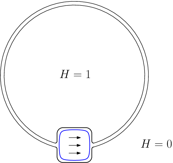
The Hamiltonian flow of is relatively slow inside the disk and fast within the pipe. For an appropriate choice of a smoothing of there exists such that is a fixed set of the time- map of the flow of . The energy is at most and depends on the area of the pipe and a choice of smoothing and can be made arbitrarily small.
We cut off inside the circle so that it is supported in a small neighborhood of the disk and the pipe. Note that this cutoff does not affect the flow of in the disk and the pipe. This construction can be copied to any symplectic surface given a disk and a simple curve which connects boundary points of the disk and does not intersect it away from the endpoints. This implies the following result.
Lemma 4.
Suppose that is represented by a simple loop. Then .
Proof.
Let be a simple loop representing . As in the previous subsection, we deform so that there exists a disk of area whose boundary points are connected by an arc of and this arc does not intersect the disk except for the endpoints. An application of the Hamiltonian described above implies . The lemma follows by letting and from the fact that . ∎
Corollary 5.
Let be the set of classes represented by simple loops. It is easy to see that generates . Denote by the norm on given by word length with respect to . The triangle inequality implies . The same argument holds also for the homotopical length spectrum.
Given any surface , admits a basis represented by simple loops. By the triangle inequality, where is the word length norm with respect to . is a homogeneous norm on . This shows the upper bound for the third case in Theorem 1. A more careful argument may provide better constants. For example, in the case of an annulus the bound can be improved to
(see [Kha1]).
Lemma 6.
Let be a surface with positive genus. Then every homology class in can be represented by a sum of two simple loops.
Proof.
Step 1: Suppose is a torus. and generate . Any class can be decomposed into the sum
where each summand is represented by a simple loop (see Figure 6).

Step 2: Suppose is a punctured torus. Without loss of generality we assume that all punctures lie on a horizontal meridian. admits a basis of vertical meridians and a horizontal meridian (see Figure 7). Then every
admits a decomposition
where each summand is represented by a simple loop.

Step 3: Suppose . can be decomposed into a connected sum of punctured tori
We identify with their image in by abuse of notation.
![[Uncaptioned image]](1411.2219v1/surfcut.jpg)
Pick . There exist such that . By the previous step we choose homology classes represented by simple loops such that . Now
Both and are represented by simple loops: consider a connected sum of the corresponding simple loops in each . The result is a simple loop in since are disjoint. ∎
3. Construction of quasimorphisms
Let be a group. A function is called a quasimorphism if there exists a constant such that for all . is called the defect of . The quasimorphism is homogeneous if it satisfies for all and . Any homogeneous quasimorphism satisfies for commuting elements and is invariant under conjugations.
We construct quasimorphisms described in Theorem 2. Recall that is a surface of finite type of genus zero. has finite area, so without loss of generality we rescale to get . Such is symplectomorphic to the interior of a -times punctured disk where is the rank of and .
Proposition 7.
Let be an annulus (disk with one puncture). Suppose that . Pick and choose a generator for . There exists a family of invariants that satisfy:
- •
is a homogeneous quasimorphism,
- •
is Hofer-Lipschitz and -continuous,
- •
Suppose that has an invariant disk of . Then .
contains continuum of such quasimorphisms that are linearly independent.
The proposition implies Theorem 2.
Proof of Theorem 2.
Pick such a quasimorphism and denote by
the embeddings obtained by gluing all punctures except for and identifying the resulting once punctured disk with . The pullback quasimorphisms satisfy the Lipschitz and continuity properties. Given a Hamiltonian with a fixed disk of area , counts the winding number of around . Denote by a small positively oriented circle in around which does not encircle other punctures. is a basis for . The dual basis allows us to write
for all Hamiltonians with a fixed disk as above. This implies
is a homogeneous quasimorphism which satisfies all properties of Theorem 2. Continuum of linearly independent choices of implies that for a choice of . ∎
Proof of Proposition 7 takes the rest of this section. It can be found in [Kha1], we give it below for the sake of completeness. We use notation equipped with the standard symplectic form , . Without loss of generality we assume that the generator is represented by the positively oriented circle . Let be a disk with , denote . Put to be the stabilizer of in . We denote .
Pick a function with compact support such that away from a small neighborhood of . Denote by the time- map of the Hamiltonian flow generated by . It is easy to see that with trajectory . Note that . We construct a quasimorphism .
Step I: it is sufficient to construct a homogeneous quasimorphism which satisfies:
- •
is Hofer-Lipschitz,
- •
, ,
- •
vanishes on for all disks .
Proof.
vanishes on Hamiltonians supported in a disk. It follows from the results of [EPP] that such is continuous in the -topology. Any decomposes as for some . Hence
( denotes the defect of ). It follows that
where . Note that , hence by homogenuity
which implies in the limit as .
We set . Suppose that has an invariant disk of .
- (1)
We consider the case . Then for some and
- (2)
The case . Pick such that . Then hence
- (3)
The case . Pick a smaller disk with . , choose such that . Then is a fixed disk of area for hence
We claim that . Indeed, the disk is fixed for , and their iterates. Moreover, differs from by a Hamiltonian . Hence by the homogenuity of
is bounded by the defect of . Letting we show .
∎
Step II: in order to build we use the Calabi quasimorphism on which was constructed by M. Entov and L. Polterovich in [EP]. We give a brief recollection of the relevant facts.
Let be an open disk equipped with a symplectic form . Let , be a time-dependent smooth function with compact support. We define
As is exact on , descends to a homomorphism which is called the Calabi homomorphism. Clearly, for , .
Let be a sphere equipped with a symplectic form . Suppose . For a smooth function the Reeb graph is defined as the set of connected components of level sets of (for a more detailed definition we refer the reader to [EP]). For a generic Morse function this set, equipped with the topology induced by the projection , is homeomorphic to a tree. We endow with a measure given by for any with measurable . is called a median of if the measure of each connected component of does not exceed . By [EP] a median exists and is unique. This construction can be extended to functions such that is Morse.
[EP] describes construction of a homogeneous quasimorphism . It has the following properties: is Hofer-Lipschitz (). In the case when is supported in a disk which is displaceable in , . Moreover, for generated by an autonomous function , can be computed in the following way. Let be the median of and be the corresponding subset of . Then
Given a symplectic embedding into a sphere of area , consider the pullback . Namely, given , extend to by identity on the complement of . Then . Clearly, is a homogeneous quasimorphism. It has the following properties:
- •
for any supported in a disk of area . To see that note that the corresponding is supported in a displaceable disk in .
- •
- •
for an autonomous generated by a compactly supported function ,
where is the level set component which is sent by to the median set of in .
Consider the embeddings () into a sphere of area that are given by gluing a disk of area to and a disk of area to . This construction ensures that bisects into two displaceable disks.
We pick and set
| (1) |
We claim that satisfies conditions of Step I. Obviously, is a homogeneous quasimorphism on which satisfies the Lipschitz property:
Consider the function which was used to define the Hamiltonian described above. It is easy to see that the “median” level set of which is relevant for the computation of is . Hence
This implies
Suppose that for some disk . Then
since is conjugate to .
It is left to show that vanishes on . Denote by the subgroup of which fixes a neighborhood of pointwise.
Lemma 8.
Let be a homogeneous quasimorphism which is Hofer-continuous and vanishes on . Then vanishes on .
Proof.
Pick an open disk . , therefore vanishes on . It follows from the results of [EPP] that is continuous in the -topology.
Suppose . This implies (as a set). Applying an appropriate isotopy supported near , we may ensure that on . Moreover, may be chosen with arbitrarily small Hofer norm. Further, we may find a -small diffeomorphism such that in a neighborhood of . It follows that and . Hofer- and -continuity of imply that . ∎
Let . We show that . splits to a composition where is supported in and is supported in the pair of pants . have disjoint supports, therefore they commute. Hence . Note that is supported in a disk, so .
is Hamiltonian in , but after the restriction to we have just . In the argument below we apply a sequence of deformations to in order to get whose restriction . All deformations involved in the process preserve the value . Finally, we show that by explicit computation.
The mapping class group is isomorphic to and is generated by Dehn twists near the three boundary components. For the proof of this fact we refer the reader to [FM] where the authors show that and is generated by Dehn twists. Note that are isotopic in if and only if they are isotopic in . As Dehn twists belong to , the statement for follows.
Denote by Dehn twists near , and by a Dehn twist in near . There are Hamiltonians in with arbitrary small Hofer norm whose restriction to realizes the Dehn twist . For example, consider a bump function supported near which has small height but is very steep in an annulus near . is isotopic in to some (). If we replace the original by . As can be chosen to be arbitrarily small, by continuity of it is enough to show the desired statement for the deformed . After the replacement vanishes, hence the modified . Note that is induced by a Hamiltonian . The definition of implies that (recall that is the chosen generator of ). The minus sign appears because opposite orientations of the boundary components result in the opposite directions of the corresponding Dehn twists. Moreover, as , hence . Therefore the restriction belongs to the identity component of .
Pick supported in a small neighborhood of such that in a neighborhood of the closure . Denote by the time- map generated by the Hamiltonian flow of . is supported in a disk in , hence for all .
Consider the homomorphism induced by inclusion . Both are Hamiltonian in , hence their fluxes are zero in . After restriction to , belong to one-dimensional subspace . , therefore one can find an appropriate such that restricts to with zero flux in . The results of [Ban] imply .
Pick a compactly supported function whose flow generates . Denote by the complement of the closed disk in , it is a displaceable disk. and it is supported in , therefore
is independent of . Hence . From we obtain that
is bounded by the defect of . It follows that is bounded on the subgroup . As is homogeneous, it vanishes there.
Remark.
Choice of different parameters in (1) gives rise to different quasimorphisms . If we fix and let vary, we get a linearly independent family. We show that by an argument from [BEP]: let be a function which depends only on and denote by the corresponding Hamiltonian. The median level set relevant for is , hence
If we consider the set of all Hamiltonians generated by functions , the values of the family applied to this set are linearly independent.
4. Discussion
4.1. Comparison with the Riemannian length spectrum
In the case of a Riemannian manifold the marked length spectrum contains a lot of information regarding the metric . For example, in a closed negatively curved surface , is completely determined by ( [Ota]).
The symplectic analogue looks much less rewarding. The only case when is not bounded is the case of a punctured disk. Therefore Hofer’s length spectrum is able to detect genus zero surfaces of bounded area. It may happen that more accurate estimates of provide additional information regarding the topology of .
On the other side, the symplectic setting is less rich than the Riemannian one. The equivalence class of is determined by the genus, and . In the case of finite area is just a scaling factor, hence asymptotic behavior behavior of depends only on the topology of . Clearly, is able to extract some of the topological information of . This result may be interpreted as the fact that the geometry of sees some of the topology of .
4.2. Homotopical spectrum
It would be interesting to provide similar estimates for . When we consider the asymptotical behavior of , it is more convenient to discuss the stabilized version
The homological version of is a norm on when and . In all other cases .
If we replace by , the argument from the previous sections gives the following partial information:
- •
Suppose that . Then . This is true since the argument of Section 2.1 applies for and not just .
- •
Suppose and . Assume that is represented by a simple nonseparating loop. Then can be represented by catenation of two simple loops, hence . Therefore and for all .
- •
Suppose and . If corresponds to a nonzero homology class then .
The author does not know estimates for most of the remaining cases. For example, let and . For a primitive self intersecting class the number of simple curves needed to represent is not bounded as (see [Cal]), so the argument for the upper bound does not give a lot. On the other hand, we do not know any tools that may give a nontrivial lower bound. There are several constructions of quasimorphisms on positive genus surfaces, but none of them is known to respect Hofer’s metric. When and belongs to the commutator subgroup , the argument used in this paper fails as translation by cannot be realized by an autonomous flow. It may happen that Entov-Polterovich quasimorphisms used in our argument still imply a nontrivial lower bound. Unfortunately, the author was not able to compute them on appropriate non-autonomous examples.
D. Calegari observed that if one takes the word length norm with respect to the generating set of simple loops, then times its stabilized version satisfies all properties of described above (we assume ). Indeed, the discussion in Section 2 implies and we do not know any example where the inequality is strict.
4.3. Higher dimensions
Most arguments and constructions used in this paper completely fail when one considers balls or tori in higher dimension manifolds. For example, upper bounds for were induced by decomposition of into simple loops. In dimension any loop can be perturbed into a simple one. However, we cannot translate a ball through a pipe containing such simple loop because of the ‘symplectic camel’ phenomenon.
4.4. The quasimorphism
Theorem 2 describes quasimorphisms for a times punctured disk . can be seen as a generalization of the rotation number . Indeed, satisfies the following: it is Lipschitz with respect to the -norm on . If has a fixed point , then computes the degree of the trajectory of under . In fact, is determined by the second property, while there is a continuous family if linearly independent homogeneous quasimorphisms satisfying same properties as .
Let be a Hamiltonian isotopy and a disk of area or greater. The computation in Section 3 shows that vanishes on those isotopies that fix for all . This implies that the value is determined up to a bounded defect by the trajectory . That is, for any such that , is bounded. Therefore can be thought as an invariant of Hamiltonian isotopies of .
In particular, nearly ignores those dynamical attributes that do not affect a large enough disk in , it sees only ‘global’ features that deform all large disks. In this sense it is different from most other generalizations of rotation number to dimension two.
A possible application is the ability to detect non-existence of large fixed or periodic disks. Namely, if we pick two such quasimorphisms and , then has neither fixed nor periodic disks of area . More than that, if one wishes to perturb in order to have such a periodic disk, allows to estimate a lower bound on Hofer’s energy of such perturbation. However, current techniques allow to compute the value of in very limited number of scenarios (like the case of autonomous Hamiltonians, locally supported and etc.) which limits practical use of this observation.
Another application is as follows. Pick a non-displaceable disk in and two linearly independent quasimorphisms where . Denote by the space of Lagrangians Hamiltonian isotopic to . Suppose that is a Hamiltonian isotopy. A simple computation shows that depends (up to a bounded defect) just on . This way gives rise to an invariant on which is Lipschitz with respect to the induced Hofer’s norm. is not bounded since it is a nonzero homogeneous quasimorphism, therefore by Lipschitz property the space is not bounded in Hofer’s norm as well (a similar argument with more details can be found in [Kha2]).
References
- [Ban] A. Banyaga. The structure of classical diffeomorphism groups, volume 400 of Mathematics and Its Applications. Kluwer Academic Publishers Group, Dordrecht; Boston, 1997.
- [BEP] P. Biran, M. Entov, and L. Polterovich. Calabi quasimorphisms for the symplectic ball. Commun. Contemp. Math., 6(5):793–802, 2004.
- [Cal] D. Calegari. Word length in surface groups with characteristic generating sets. Proc. Amer. Math. Soc., 136(7):2631–2637, 2008.
- [EP] M. Entov and L. Polterovich. Calabi quasimorphism and quantum homology. Int. Math. Res. Not., 2003(30):1635–1676, 2003.
- [EPP] M. Entov, L. Polterovich, and P. Py. On continuity of quasimorphisms for symplectic maps. In Perspectives in Analysis, Geometry, and Topology (a volume dedicated to Oleg Viro’s 60th birthday), volume 296 of Progress in Mathematics. Birkhäuser, Basel, 2012.
- [FM] B. Farb and D. Margalit. A Primer on Mapping Class Groups. Princeton Mathematical Series. Princeton University Press, Princeton, NJ, 2011.
- [Kha1] M. Khanevsky. Hofer’s norm and disk translations in an annulus. Can be found at arXiv:1111.1923 [math.SG].
- [Kha2] M. Khanevsky. Geometric and topological aspects of Lagrangian submanifolds - intersections, diameter and Floer theory. PhD thesis, Tel Aviv University, 2011.
- [LM] F. Lalonde and D. McDuff. Hofer’s -geometry: energy and stability of hamiltonian flows, part ii. Invent. Math., 122(1):35–�69, 1995.
- [Ota] J.-P. Otal. Le spectre marque des longueurs des surfaces a courbure negative. Annals of Math., 131:151–162, 1990.
- [Rou] F. Le Roux. Six questions, a proposition and two pictures on Hofer distance for Hamiltonian diffeomorphisms on surfaces. In Y.-G. Oh A. Fathi and C. Viterbo, editors, Symplectic Topology and Measure Preserving Dynamical Systems, volume 512 of Contemporary Mathematics, pages 33–40. Amer. Math. Soc., Providence, RI, 2010.