Multivariate $f$-Divergence Estimation With Confidence

Estimators for some $f$-divergences already exist. For example, Póczos & Schneider [8] and Wang et al [18] provided consistent $k$-nn estimators for Rényi-$\alpha$ and the KL divergences, respectively. Consistency has been proven for other mutual information and divergence estimators based on plug-in histogram schemes [19, 20, 21, 22]. Hero et al [16] provided an estimator for Rényi-$\alpha$ divergence but assumed that one of the densities was known. However none of these works study the convergence rates of their estimators nor do they derive the asymptotic distributions.

Recent work has focused on deriving convergence rates for divergence estimators. Nguyen et al [23], Singh and Póczos [24], and Krishnamurthy et al [25] each proposed divergence estimators that achieve the parametric convergence rate ($O\left(\frac{1}{T}\right)$) under weaker conditions than those given in [1]. However, solving the convex problem of [23] can be more demanding for large sample sizes than the estimator given in [1] which depends only on simple density plug-in estimates and an offline convex optimization problem. Singh and Póczos only provide an estimator for Rényi-$\alpha$ divergences that requires several computations at each boundary of the support of the densities which becomes difficult to implement as $d$ gets large. Also, this method requires knowledge of the support of the densities which may not be possible for some problems. In contrast, while the convergence results of the estimator in [1] requires the support to be bounded, knowledge of the support is not required for implementation. Finally, the estimators given in [25] estimate divergences that include functionals of the form $\int f_{1}^{\alpha}(x)f_{2}^{\beta}(x)d\mu(x)$ for given $\alpha,\,\beta$. While a suitable $\alpha$-$\beta$ indexed sequence of divergence functionals of the form in [25] can be made to converge to the KL divergence, this does not guarantee convergence of the corresponding sequence of divergence estimates, whereas the estimator in [1] can be used to estimate the KL divergence. Also, for some divergences of the specified form, numerical integration is required for the estimators in [25], which can be computationally difficult. In any case, the asymptotic distributions of the estimators in [23, 24, 25] are currently unknown.

Asymptotic normality has been established for certain appropriately normalized divergences between a specific density estimator and the true density [26, 27, 28]. However, this differs from our setting where we assume that both densities are unknown. Under the assumption that the two densities are smooth, lower bounded, and have bounded support, we show that an appropriately normalized weighted ensemble average of kernel density plug-in estimators of $f$-divergence converges in distribution to the standard normal distribution. This is accomplished by constructing a sequence of interchangeable random variables and then showing (by concentration inequalities and Taylor series expansions) that the random variables and their squares are asymptotically uncorrelated. The theory developed to accomplish this can also be used to derive a central limit theorem for a weighted ensemble estimator of entropy such as the one given in [3].We verify the theory by simulation. We then apply the theory to the practical problem of empirically bounding the Bayes classification error probability between two population distributions, without having to construct estimates for these distributions or implement the Bayes classifier.

Bold face type is used in this paper for random variables and random vectors. Let $f_{1}$ and $f_{2}$ be densities and define $L(x)=\frac{f_{1}(x)}{f_{2}(x)}$. The conditional expectation given a random variable $\mathbf{Z}$ is $\mathbb{E}_{\mathbf{Z}}$.

The full proof is included in the appendices. We use the following lemma from [30, 31]:

This lemma is an extension of work by Blum et al [32] which showed that if $\left\{\mathbf{Z}_{i};i=1,2,\dots\right\}$ is an interchangeable process with zero mean and unit variance, then $\mathbf{S}_{N}=\frac{1}{\sqrt{N}}\sum_{i=1}^{N}\mathbf{Z}_{i}$ converges in distribution to a standard normal random variable if and only if $Cov\left[\mathbf{Z}_{1},\mathbf{Z}_{2}\right]=0$ and $Cov\left[\mathbf{Z}_{1}^{2},\mathbf{Z}_{2}^{2}\right]=0$. In other words, the central limit theorem holds if and only if the interchangeable process is uncorrelated and the squares are uncorrelated. Lemma 3 shows that for a correlated interchangeable process, a sufficient condition for a central limit theorem is for the interchangeable process and the squared process to be asymptotically uncorrelated with rate $O(1/M)$.

For simplicity, let $M_{1}=M_{2}=M$ and $\hat{\mathbf{L}}_{k(l)}:=\hat{\mathbf{L}}_{k(l),k(l)}$. Define

Then from Eq. 4, we have that

Thus it is sufficient to show from Lemma 3 that $Cov(\mathbf{Y}_{M,1},\mathbf{Y}_{M,2})$ and $Cov(\mathbf{Y}_{M,1}^{2},\mathbf{Y}_{M,2}^{2})$ are $O(1/M)$. To do this, it is necessary to show that the denominator of $\mathbf{Y}_{M,i}$ converges to a nonzero constant or to zero sufficiently slowly. It is also necessary to show that the covariance of the numerator is $O(1/M)$. Therefore, to bound $Cov(\mathbf{Y}_{M,1},\mathbf{Y}_{M,2})$, we require bounds on the quantity $Cov\left[g\left(\hat{\mathbf{L}}_{k(l)}(\mathbf{X}_{i})\right),g\left(\hat{\mathbf{L}}_{k(l^{\prime})}(\mathbf{X}_{j})\right)\right]$ where $l,\,l^{\prime}\in\bar{l}$.

Define $\mathcal{M}(\mathbf{Z}):=\mathbf{Z}-\mathbb{E}\mathbf{Z}$, $\hat{\mathbf{F}}_{k(l)}(\mathbf{Z}):=\hat{\mathbf{L}}_{k(l)}(\mathbf{Z})-\mathbb{E}_{\mathbf{Z}}\left(\hat{\mathbf{L}}_{k(l)}(\mathbf{Z})\right)$, and $\hat{\mathbf{e}}_{i,k(l)}(\mathbf{Z}):=\hat{\mathbf{f}}_{i,k(l)}(\mathbf{Z})-\mathbb{E}_{\mathbf{Z}}\hat{\mathbf{f}}_{i,k(l)}(\mathbf{Z})$. Assuming $g$ is sufficiently smooth, a Taylor series expansion of $g\left(\hat{\mathbf{L}}_{k(l)}(\mathbf{Z})\right)$ around $\mathbb{E}_{\mathbf{Z}}\hat{\mathbf{L}}_{k(l)}(\mathbf{Z})$ gives

where $\mathbf{\xi_{Z}}\in\left(\mathbb{E}_{\mathbf{Z}}\hat{\mathbf{F}}_{k(l)}(\mathbf{Z}),\hat{\mathbf{F}}_{k(l)}(\mathbf{Z})\right)$. We use this expansion to bound the covariance. The expected value of the terms containing the derivatives of $g$ is controlled by assuming that the densities are lower bounded. By assuming the densities are sufficiently smooth, an expression for $\hat{\mathbf{F}}_{k(l)}^{q}\left(\mathbf{Z}\right)$ in terms of powers and products of the density error terms $\hat{\mathbf{e}}_{1,k(l)}$ and $\hat{\mathbf{e}}_{2,k(l)}$ is obtained by expanding $\hat{\mathbf{L}}_{k(l)}(\mathbf{Z})$ around $\mathbb{E}_{\mathbf{Z}}\hat{\mathbf{f}}_{1,k(l)}(\mathbf{Z})$ and $\mathbb{E}_{\mathbf{Z}}\hat{\mathbf{f}}_{2,k(l)}(\mathbf{Z})$ and applying the binomial theorem. The expected value of products of these density error terms is bounded by applying concentration inequalities and conditional independence. Then the covariance between $\hat{\mathbf{F}}_{k(l)}^{q}(\mathbf{Z})$ terms is bounded by bounding the covariance between powers and products of the density error terms by applying Cauchy-Schwarz and other concentration inequalities. This gives the following lemma which is proved in the appendices.

Note that $k(l)$ is required to grow with $\sqrt{M}$ for Lemma 4 to hold. Define $h_{l,g}(\mathbf{X})=g\left(\mathbb{E}_{\mathbf{X}}\hat{\mathbf{L}}_{k(l)}(\mathbf{X})\right)$. Lemma 4 can then be used to show that

For the covariance of $\mathbf{Y}_{M,i}^{2}$ and $\mathbf{Y}_{M,j}^{2}$, assume WLOG that $i=1$ and $j=2$. Then for $l,\,l^{\prime},\,j,\,j^{\prime}$ we need to bound the term

For the case where $l=l^{\prime}$ and $j=j^{\prime}$, we can simply apply the previous results to the functional $d(x)=\left(\mathcal{M}\left(g(x)\right)\right)^{2}$. For the more general case, we need to show that

To do this, bounds are required on the covariance of up to eight distinct density error terms. Previous results can be applied by using Cauchy-Schwarz when the sum of the exponents of the density error terms is greater than or equal to 4. When the sum is equal to 3, we use the fact that $k(l)=O(k(l^{\prime}))$ combined with Markov’s inequality to obtain a bound of $O\left(1/M\right)$. Applying Eq. 6 to the term in Eq. 5 gives the required bound to apply Lemma 3.

To the best of our knowledge, Theorem 2 provides the first results on the asymptotic distribution of an $f$-divergence estimator with MSE convergence rate of $O\left(1/T\right)$ under the setting of a finite number of samples from two unknown, non-parametric distributions. This enables us to perform inference tasks on the class of $f$-divergences (defined with smooth functions $g$) on smooth, strictly lower bounded densities with finite support. Such tasks include hypothesis testing and constructing a confidence interval on the error exponents of the Bayes probability of error for a classification problem. This greatly increases the utility of these divergence estimators.

Although we focused on a specific divergence estimator, we suspect that our approach of showing that the components of the estimator and their squares are asymptotically uncorrelated can be adapted to derive central limit theorems for other divergence estimators that satisfy similar assumptions (smooth $g$, and smooth, strictly lower bounded densities with finite support). We speculate that this would be easiest for estimators that are also based on $k$-nearest neighbors such as in [8] and [18]. It is also possible that the approach can be adapted to other plug-in estimator approaches such as in [24] and [25]. However, the qualitatively different convex optimization approach of divergence estimation in [23] may require different methods.

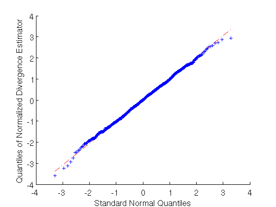
To verify the central limit theorem of the ensemble method, we estimated the KL divergence between two truncated normal densities restricted to the unit cube. The densities have means $\bar{\mu}_{1}=0.7*\bar{1}_{d}$, $\bar{\mu}_{2}=0.3*\bar{1}_{d}$ and covariance matrices $\sigma_{i}I_{d}$ where $\sigma_{1}=0.1,$ $\sigma_{2}=0.3,$ $\bar{1}_{d}$ is a $d$-dimensional vector of ones, and $I_{d}$ is a $d$-dimensional identity matrix. We show the Q-Q plot of the normalized optimally weighted ensemble estimator of the KL divergence with $d=6$ and $1000$ samples from each density in Fig. 1. The linear relationship between the quantiles of the normalized estimator and the standard normal distribution validates Theorem 2.

Our ensemble divergence estimator can be used to estimate a bound on the Bayes probability of error [7]. Suppose we have two classes $C_{1}$ or $C_{2}$ and a random observation $x$. Let the a priori class probabilities be $w_{1}=Pr(C_{1})>0$ and $w_{2}=Pr(C_{2})=1-w_{1}>0$. Then $f_{1}$ and $f_{2}$ are the densities corresponding to the classes $C_{1}$ and $C_{2}$, respectively. The Bayes decision rule classifies $x$ as $C_{1}$ if and only if $w_{1}f_{1}(x)>w_{2}f_{2}(x)$. The Bayes error $P_{e}^{*}$ is the minimum average probability of error and is equivalent to

where $p(x)=w_{1}f_{1}(x)+w_{2}f_{2}(x)$. For $a,\,b>0$, we have

Replacing the minimum function in Eq. 7 with this bound gives

where $c_{\alpha}(f_{1}||f_{2})=\int f_{1}^{\alpha}(x)f_{2}^{1-\alpha}(x)dx$ is the Chernoff $\alpha$-coefficient. The Chernoff coefficient is found by choosing the value of $\alpha$ that minimizes the right hand side of Eq. 8:

Thus if $\alpha^{*}=\arg\min_{\alpha\in(0,1)}c_{\alpha}(f_{1}||f_{2})$, an upper bound on the Bayes error is

Equation 9 includes the form in Eq. 1 ($g(x)=x^{\alpha}$). Thus we can use the optimally weighted ensemble estimator described in Sec. 2 to estimate a bound on the Bayes error. In practice, we estimate $c_{\alpha}(f_{1}||f_{2})$ for multiple values of $\alpha$ (e.g. $0.01,0.02,\dots,0.99$) and choose the minimum.

We estimated a bound on the pairwise Bayes error between the three classes (Setosa, Versicolor, and Virginica) in the Iris data set [33, 34] and used bootstrapping to calculate confidence intervals. We compared the bounds to the performance of a quadratic discriminant analysis classifier (QDA) with 5-fold cross validation. The pairwise estimated 95% confidence intervals and the misclassification rates of the QDA are given in Table 1. Note that the right endpoint of the confidence interval is less than $1/50$ when comparing the Setosa class to either of the other two classes. This is consistent with the performance of the QDA and the fact that the Setosa class is linearly separable from the other two classes. In contrast, the right endpoint of the confidence interval is higher when comparing the Versicolor and Virginica classes which are not linearly separable. This is also consistent with the QDA performance. Thus the estimated bounds provide a measure of the relative difficulty of distinguishing between the classes, even though the small number of samples for each class ($50$) limits the accuracy of the estimated bounds.

References

• [1] K. R. Moon and A. O. Hero III, “Ensemble estimation of multivariate f-divergence,” in IEEE International Symposium on Information Theory, pp. 356–360, 2014.
• [2] K. Sricharan and A. O. Hero III, “Ensemble weighted kernel estimators for multivariate entropy estimation,” in Adv. Neural Inf. Process. Syst., pp. 575–583, 2012.
• [3] K. Sricharan, D. Wei, and A. O. Hero III, “Ensemble estimators for multivariate entropy estimation,” IEEE Trans. on Inform. Theory, vol. 59, no. 7, pp. 4374–4388, 2013.
• [4] I. Csiszar, “Information-type measures of difference of probability distributions and indirect observations,” Studia Sci. Math. Hungar., vol. 2, pp. 299–318, 1967.
• [5] S. Kullback and R. A. Leibler, “On information and sufficiency,” The Annals of Mathematical Statistics, vol. 22, no. 1, pp. 79–86, 1951.
• [6] A. Rényi, “On measures of entropy and information,” in Fourth Berkeley Sympos. on Mathematical Statistics and Probability, pp. 547–561, 1961.
• [7] T. M. Cover and J. A. Thomas, Elements of Information Theory. John Wiley & Sons, 2006.
• [8] B. Póczos and J. G. Schneider, “On the estimation of alpha-divergences,” in International Conference on Artificial Intelligence and Statistics, pp. 609–617, 2011.
• [9] J. B. Oliva, B. Póczos, and J. Schneider, “Distribution to distribution regression,” in International Conference on Machine Learning, pp. 1049–1057, 2013.
• [10] I. S. Dhillon, S. Mallela, and R. Kumar, “A divisive information theoretic feature clustering algorithm for text classification,” The Journal of Machine Learning Research, vol. 3, pp. 1265–1287, 2003.
• [11] H. Peng, F. Long, and C. Ding, “Feature selection based on mutual information criteria of max-dependency, max-relevance, and min-redundancy,” Pattern Analysis and Machine Intelligence, IEEE Transactions on, vol. 27, no. 8, pp. 1226–1238, 2005.
• [12] B. Chai, D. Walther, D. Beck, and L. Fei-Fei, “Exploring functional connectivities of the human brain using multivariate information analysis,” in Adv. Neural Inf. Process. Syst., pp. 270–278, 2009.
• [13] J. Lewi, R. Butera, and L. Paninski, “Real-time adaptive information-theoretic optimization of neurophysiology experiments,” in Adv. Neural Inf. Process. Syst., pp. 857–864, 2006.
• [14] E. Schneidman, W. Bialek, and M. J. Berry, “An information theoretic approach to the functional classification of neurons,” in Adv. Neural Inf. Process. Syst., pp. 197–204, 2002.
• [15] K. M. Carter, R. Raich, and A. O. Hero III, “On local intrinsic dimension estimation and its applications,” Signal Processing, IEEE Transactions on, vol. 58, no. 2, pp. 650–663, 2010.
• [16] A. O. Hero III, B. Ma, O. J. Michel, and J. Gorman, “Applications of entropic spanning graphs,” Signal Processing Magazine, IEEE, vol. 19, no. 5, pp. 85–95, 2002.
• [17] K. R. Moon and A. O. Hero III, “Ensemble estimation of multivariate f-divergence,” CoRR, vol. abs/1404.6230, 2014.
• [18] Q. Wang, S. R. Kulkarni, and S. Verdú, “Divergence estimation for multidimensional densities via k-nearest-neighbor distances,” IEEE Trans. Inform. Theory, vol. 55, no. 5, pp. 2392–2405, 2009.
• [19] G. A. Darbellay, I. Vajda, et al., “Estimation of the information by an adaptive partitioning of the observation space,” IEEE Trans. Inform. Theory, vol. 45, no. 4, pp. 1315–1321, 1999.
• [20] Q. Wang, S. R. Kulkarni, and S. Verdú, “Divergence estimation of continuous distributions based on data-dependent partitions,” IEEE Trans. Inform. Theory, vol. 51, no. 9, pp. 3064–3074, 2005.
• [21] J. Silva and S. S. Narayanan, “Information divergence estimation based on data-dependent partitions,” Journal of Statistical Planning and Inference, vol. 140, no. 11, pp. 3180–3198, 2010.
• [22] T. K. Le, “Information dependency: Strong consistency of Darbellay–Vajda partition estimators,” Journal of Statistical Planning and Inference, vol. 143, no. 12, pp. 2089–2100, 2013.
• [23] X. Nguyen, M. J. Wainwright, and M. I. Jordan, “Estimating divergence functionals and the likelihood ratio by convex risk minimization,” IEEE Trans. Inform. Theory, vol. 56, no. 11, pp. 5847–5861, 2010.
• [24] S. Singh and B. Póczos, “Generalized exponential concentration inequality for Rényi divergence estimation,” in International Conference on Machine Learning, pp. 333–341, 2014.
• [25] A. Krishnamurthy, K. Kandasamy, B. Póczos, and L. Wasserman, “Nonparametric estimation of Rényi divergence and friends,” in International Conference on Machine Learning, vol. 32, 2014.
• [26] A. Berlinet, L. Devroye, and L. Györfi, “Asymptotic normality of L1 error in density estimation,” Statistics, vol. 26, pp. 329–343, 1995.
• [27] A. Berlinet, L. Györfi, and I. Dénes, “Asymptotic normality of relative entropy in multivariate density estimation,” Publications de l’Institut de Statistique de l’Université de Paris, vol. 41, pp. 3–27, 1997.
• [28] P. J. Bickel and M. Rosenblatt, “On some global measures of the deviations of density function estimates,” The Annals of Statistics, pp. 1071–1095, 1973.
• [29] D. O. Loftsgaarden and C. P. Quesenberry, “A nonparametric estimate of a multivariate density function,” The Annals of Mathematical Statistics, pp. 1049–1051, 1965.
• [30] K. Sricharan, R. Raich, and A. O. Hero III, “Estimation of nonlinear functionals of densities with confidence,” IEEE Trans. Inform. Theory, vol. 58, no. 7, pp. 4135–4159, 2012.
• [31] K. Sricharan, Neighborhood graphs for estimation of density functionals. PhD thesis, Univ. Michigan, 2012.
• [32] J. Blum, H. Chernoff, M. Rosenblatt, and H. Teicher, “Central limit theorems for interchangeable processes,” Canad. J. Math, vol. 10, pp. 222–229, 1958.
• [33] K. Bache and M. Lichman, “UCI machine learning repository,” 2013.
• [34] R. A. Fisher, “The use of multiple measurements in taxonomic problems,” Annals of eugenics, vol. 7, no. 2, pp. 179–188, 1936.
• [35] Y. Mack and M. Rosenblatt, “Multivariate k-nearest neighbor density estimates,” Journal of Multivariate Analysis, vol. 9, no. 1, pp. 1–15, 1979.