Properties of the flow on a polygonal Andreev billiardThanks: The work of R. G. Niemeyer was partially supported by the National Science Foundation under the MCTP grant DMS-1148801, while a postdoctoral fellow at the University of New Mexico, Albuquerque.

A classical billiard, denoted by $\Omega(B)$ where the boundary of $\Omega(B)$ is $B$, is a compact region in the plane. The boundary $B$ is sufficiently smooth so as to allow the classical law of reflection¹¹ 1 The angle of incidence $\theta_{i}$ is equal to the angle of reflection $\theta_{r}$. to hold at all but finitely many points, and a pointmass traversing the billiard does so with unit speed, zero friction and makes perfectly elastic collisions in the boundary $B$ (reflecting according to the law of reflection); see Figure 3.

The immediate goal of this paper is to rigorously define the notion of Andreev reflection as inspired by the physical phenomenon by the same name, which we now briefly describe; [Bee2] for an excellent survey of the topic of Andreev billiards from the physical perspective; additionally, see [Bee1, Bee2, BerBarBee, GooJacBee, MiPiMacBee, Wi] and the relevant references therein for the state of the art of Andreev reflection in nanowires and other physical settings. At the nanoscale—this being on the order of magnitude $10^{-9}$---quantum effects become relevant and certain concessions must be made when modeling nanoscale systems.⁶⁶ 6 Such models are semi-classical in nature. The specific setting from which this paper draws inspiration is that of a toy model of nanowire (a string of molecules much longer than tall) resting upon a superconducting plate. As one investigates the behavior of an electron (modeled as a pointmass) in a field of electrons, he or she assumes an electron obeys the law of reflection at the top of the ‘wire’ and then collides in the bottom of the ‘wire,’ and subsequently disappears. The electron does not truly disappear (nor does it truly strictly obey the law of reflection), but is pulled from the nanowire and forced to pair with another electron, this newly formed pair of electrons being called a Cooper pair; see Figure 2 for an illustration of an idealization of this phenomenon. It is worth noting that this toy model is valid when the energy in the system is the Fermi energy, this being an important requirement in the study of the solid state physics of metallic substances and superconductors. Specifically, retro-reflection will not occur when the energy of the system is not the Fermi energy.⁷⁷ 7 The author would like to thank Carlo Beenakker for pointing out these facts in previous drafts.

In the absence of the electron, the ‘stationary’ electrons⁸⁸ 8 Of course, no electron is ever stationary. We are indeed imposing many simplifications on the physical system when deriving a mathematical construct. react to the departure of the electron by exhibiting a wave (visually speaking) around the hole that gives the illusion that the hole is moving back along the trajectory of the electron. The hole then eventually collides into the bottom of the wire, whereupon an electron is pulled back into the nanowire; see Figure 3.

Seeking to reigorously define (mathematical) Andreev reflection, in our idealized setting, we will assign a parity to a pointmass. The pointmass begins with positive parity. Upon intersecting with the Andreev subset of an Andreev billiard (both of which to be formally defined in §2), the parity reverses and becomes negative, much like how the departure of an electron from a nanowire results in a hole. Subsequent collisions in the Andreev subset cause the parity to change from negative to positive and from positive to negative.

The second goal is twofold: 1) to rigorously define an Andreev billiard and 2) rigorously define the continuous and discrete flows on an Andreev billiard.

Once we have rigorously defined an Andreev billiard, we will show that the continuous and discrete flows (as defined) will preserve the essence of an Andreev billiard, namely, the continuous flow will negate the volume form $dx\wedge dy\wedge d\theta$ when intersecting with the Andreev subset and the discrete flow will preserve the measure $\cos\phi drd\phi$.

The third goal will be to examine the properties of the continuous/discrete flow. That is, we will show that under certain conditions, for almost every initial direction, the flow on almost any polygonal Andreev billiard will be closed.

Finally, taking motivation from experimental investigations of physical Andreev billiards, we will investigate the effect of a fractal perturbation a toy model of a rectangular Andreev billiard.

The paper is organized as follows. In §2, the physics of an Andreev billiard is described and rigorous definitions of mathematical Andreev reflection and polygonal Andreev billiard are given. The continuous flow $\Phi_{\pm}^{t}$ on a polygonal Andreev billiard is described in §3 and it is there that one sees that the absolute value of the volume element on the phase space of the billiard is preserved. In fact, the parity of the billiard ball of physical Andreev billiard is reflected in the fact that the volume element changes sign under the flow $\Phi_{\pm}^{t}$. In §4, the discrete flow is described and is shown to preserve the measure $\cos\phi d\phi dr$ on a section of the phase space. Finally, in §5, an investigation of the effects of a fractal perturbation of the toy model of a physical Andreev billiard is made. The reason for this investigation is to present theoretic evidence in support of the argument that certain rough boundaries of physical Andreev billiards can be first studied as fractally perturbed boundaries. A discussion of the results is then given and directions for future research are discussed.

We begin with a definition, with the end goal being a rigorous definition for Andreev reflection (given in the form of an equivalence relation $\sim_{\pm}$) and an Andreev billiard.

Heuristically speaking, a pointmass has experienced Andreev reflection if the parity of the pointmass has changed upon retro-reflecting. We define this formally as follows.

Define $\Omega(B^{+})$ (or $\Omega(B^{-})$) to be the billiard with piecewise smooth boundary $B^{+}$ (resp., $B^{-}$). $\Omega(B^{+})$ and $\Omega(B^{-})$ are billiards, whereupon the classical billiard dynamics are defined (excluding corners and cusps). Let $A^{+}$ and $A^{-}$ be nonempty subsets of $B^{+}$ and $B^{-}$, respectively, containing no singularities of the billiard flow $\Phi_{+}$ defined on $(\Omega(B^{+})\times S^{1})/\sim$ and $\Phi_{-}$ defined on $(\Omega(B^{-})\times S^{1})/\sim$, where $\sim$ is the standard relation identifying inward and outward pointing vectors on the boundary of a billiard. That is, at each point $\mathbf{x}=(x_{1},x_{2})$ of the boundary of a billiard, $(\mathbf{x},\theta)$ is identified with $(\mathbf{x},\gamma)$, where $\gamma=r(\theta)$, $r(\theta)$ being the reflection of $\theta$ through the tangent line through $\mathbf{x}$. Further assume that $B^{-}=\rho(B^{+})$, where $\rho$ is the reflection through a line parallel to $A^{+}$. Consequently, it is the case that $A^{-}=\rho(A^{+})$. Without loss of generality, we may assume $A^{+}$ and $A^{-}$ are vertical segments in their respective billiards.⁹⁹ 9 Recall that we are restricting our attention to sets in the plane with polygonal boundary.

First note that $X^{\circ}$ denotes the interior of a set $X$. Define $\sim_{\pm}$ on $(\Omega(B^{+})\cup\Omega(B^{-}))\times S^{1}$ as follows: $(\mathbf{x},\theta)\sim_{\pm}(\mathbf{y},\gamma)$ if and only if

• •

  $\mathbf{x},\mathbf{y}\in\Omega(B^{+})^{\circ}\cup\Omega(B^{-})^{\circ}$ and $(\mathbf{x},\theta)=(\mathbf{y},\gamma)$

  or

• •

  $\mathbf{x},\mathbf{y}\in(B^{+}\cup B^{-})\setminus(A^{+}\cup A^{-})$ and $\mathbf{x}=\mathbf{y}$ and

  • –

    $\theta=\gamma$ or

  • –

    $\theta=r(\gamma)$

  or

• •

  $\mathbf{x},\mathbf{y}\in A^{+}\cup A^{-}$ and

  • –

    $\mathbf{x}=\mathbf{y}$ and $\theta=\gamma$ or

  • –

    $\mathbf{x}=\rho(\mathbf{y})$ and $\theta=r(\gamma)+\pi$

The relation $\sim_{\pm}$ is an equivalence relation on $\Omega(B^{+})\cup\Omega(B^{-})\times S^{1}$. As in the classical case, we choose the representative element of an equivalence class to be the ordered pair $(\mathbf{x},\theta)$, where $\theta$ is an inward pointing direction based at $\mathbf{x}$. We now formally define Andreev billiard.

Really, the Andreev subset is two subsets of the two copies of a polygonal billiard properly identified. Upon identifying point-angle pairs, one sees that the $A^{+}$ and $A^{-}$ are effectively the same in the phase space $\Omega(B^{\pm})\times S^{1}/\sim_{\pm}$.

Figure 7 gives an example of an orbit of an Andreev billiard; the same orbit is illustrated as in Figure 6, but, as we will see, is given by a well-defined flow on $\Omega(B^{\pm})\times S^{1}/\sim_{\pm}$.

The fact that the volume element changes sign captures the essence of the physical Andreev reflection in the toy model: the pointmass represents either an electron or a hole, and what the pointmass represents changes each time with a ‘collision’ in the Andreev subset. More precisely, in the physical toy model, there is a particular parity: hole or electron. In our rigorously defined setting, we see that the volume of an open set $X$ contained in the interior of $\Omega(B^{+})$ will be negated as (and if) $\Phi^{t}$ transports $X$ into $\Omega(B^{-})$. That is, if in a fixed direction $\theta$, $\Phi^{t}(X)\subseteq\Omega(B^{-})^{\circ}$, then the volume of $\Phi^{t}(X)$ in $\Omega(B^{-})$ will be opposite that of the volume of $X$, much like how an electron colliding with the Andreev subset (the side lying upon a superconducting medium), is replaced by a hole and such a hole is then subsequently replaced by another electron. Again, one observes a physical phenomenon and attempts to construct a rigorous mathematical setting in which the toy model of such a physical setting is rigorously described. The volume parity of a set rigorously captures the electron-hole parity observed in the toy model.

The collision map $F_{\pm}:(B^{\pm}\times S^{1})/\sim_{\pm}\to(B^{\pm}\times S^{1})/\sim_{\pm}$ (when such a map is defined), preserves the measure $\cos\phi drd\phi$. The derivative of $F_{\pm}$ is entirely dependent on the curvature of the segments comprising $B^{+}$ and $B^{-}$ and the initial direction $\theta$. We then denote the parameterization of the side on which $(\bar{x}^{\prime},\bar{y}^{\prime})$ lies by $r^{\prime}$; see Figure 9.

Figure 9 demonstrates how a pointmass is reflected in the Andreev subset of $\Omega(B^{\pm})$.¹¹¹¹ 11 More precisely, $A^{+}$ and $A^{-}$ have been identified in the phase space. The subset $A^{+}$ (or $A^{-}$) has a parametrization given by $r$. We note that $\theta$ is the direction of the trajectory, $\theta^{\prime}$ the angle at which the pointmass is reflected off of $r^{\prime}$. The angles $\theta$ and $\theta^{\prime}$ are measured relative to positive horizontal axis, as shown. The angles $\gamma$ and $\gamma^{\prime}$ measure the angle between the positive horizontal axis and the sides $r$ and $r^{\prime}$, respectively. The angles $\psi$ and $\psi^{\prime}$ measure the angle between $r$ and $r^{\prime}$, respectively.

The following is motivated by the toy model of the physical setting of the electron-hole dynamics in a metallic nanowire with three “sides” of the wire exhibiting the standard law of reflection and the other being the superconducting side, as illustrated in Figure 4. We give examples where particular perturbations may pose a problem for reliably modeling the dynamics of the electron-hole flow in a nanowire.

Consider a toy model of a physical rectangular Andreev billiard $\Omega(R)$ with rationally commensurate side lengths (the ratio of the lengths of any two sides is a rational value) and the base of $\Omega(R)$ being the subset of $R$ at which retro-reflection with parity occurs; see Figures 2–4 for a reminder of exactly how the toy model for physical Andreev reflection is behaving.

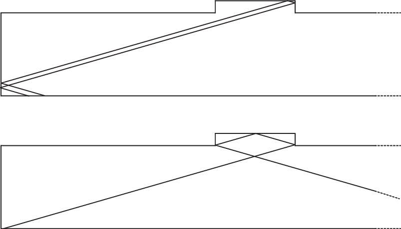
Consider the perturbation of $\Omega(R)$ given in Figure 10. The effect of perturbing the wire by introducing this rectangular region is shown in Figure 11. We see in Figure 11 that the perturbation of the side has the effect of forcing the billiard ball back along a path in the same direction of its entry or along the direction as expected in the absence of the perturbation, depending on where the billiard ball began. Indeed, for any direction, one can construct a rectangular perturbation where the choice of initial base point results in the perturbation affecting the billiard ball differently.

In [LapMilNie], billiard dynamics on the so-called $T$-fractal billiard $\Omega(\mathscr{T})$ are studied; see Figure 12.¹³¹³ 13 To the best of the author’s knowledge, the $T$-fractal was first introduced in [AcST]. The $T$-fractal billiard is not a classical billiard; it is a fractal billiard as discussed in [LapNie1, LapNie2, LapNie3, LapNie4]. However, in particular rational directions (of which there are countably infinitely many), one can determine periodic orbits of $\Omega(\mathscr{T})$. Such orbits reach the top of the $T$-fractal billiard $\Omega(\mathscr{T})$, and, effectively retro-reflect, but without a change in parity. Upon returning to the bottom of the fractal billiard, the ball continues accordingly; see, e.g., Figure 13. Specifically, Theorem 4.9 in [LapMilNie] describes a countable family of directions and a dense set of initial basepoints from which one can construct a periodic degenerate orbit of the $T$-fractal billiard. We restate the theorem here for the reader’s easy reference.

Suppose we consider a perturbation of a nanowire in the shape of the $T$-fractal billiard $\Omega(\mathscr{T})$. Supposing we consider an electron-hole (or a billiard ball with parity) entering into such a perturbation at a point and with an initial direction described in the hypotheses of Theorem 4, then such a perturbation will cause the electron-hole to return to the rectangular region of the nanowire antiparallel to the direction in which it entered, this being discussed in the proof of Theorem 4.9 in [LapMilNie]. This sort of perturbation causes the orbit of the nanowire to behave as if the electron-hole had intersected a vertical side at or near the corner of the nanowire; see Figure 14 and Figure 15.

To be clear, never¹⁴¹⁴ 14 in any reasonable amount of time will anyone be able to perturb a nanowire in such a way that the $T$-fractal appears, simply because the $T$-fractal is only a set that exists in one’s mind. For that matter, and for all intents and purposes, any approximation of the $T$-fractal is not a reasonable or realistic perturbation of a rectangular nanowire. Nevertheless, whether it be in a physical setting or an abstract setting, one may find the existence of a fractal perturbation interesting in its own right or inspiring some other train of thought not yet foreseen by the author. The argument made in this paper is that a rectangular billiard is a reasonable approximation to a nanowire and that the evidence of a particular perturbation mimicking the severing of a nanowire may highlight a new perturbation worth examining on the physical side of the subject, if perhaps only in computer simulations.

From §3, it is clear that the flow on a rational polygonal Andreev billiard in almost any direction will be closed. The volume parity discussed in §3 is analogous to the electron-hole parity modeled in Figures 2 and 3. As expected, however, the discrete flow $F_{\pm}^{n}$ preserves the measure $\cos\phi d\phi dr$ on the space $(\Omega(B^{\pm})\times S^{1})/\sim_{\pm}$.

In returning to the toy model, a discussion of perturbations of a nanowire was given in §5. It was there that the $T$-fractal was shown to effectively sever a nanowire by forcing all trajectories in a particular fixed direction to retroreflect back into the rectangular region. Such a theoretical investigation sought to shed light on the idea that fractal perturbations of polygonal billiard tables (esp., polygonal Andreev billiard tables) are meaningful.

Much of this article has been on the topic of polygonal Andreev billiards. One can reasonably expect the same rigorously defined Andreev reflection to carry over to a more general setting where the boundary of an Andreev billiard is not the union of two polygonal billiards but two copies of a piecewise smooth curve properly identified. With suitable adjustments to the construction of an Andreev billiard, one can then discuss a more general Andreev billiard, analyze the flow and determine whether or not in almost any direction the flow would remain closed. It is unlikely that the flow in almost any direction on an arbitrary Andreev billiard will be closed since there are known examples of billiard tables whereupon the flow is not equidistributed nor minimal; see [Sm]. Additionally, it is conceivable that there exists a billiard such that for some fixed direction $\theta$, every orbit is not closed, but also not dense, meaning the orbit gets trapped in some proper subset of the table.

Future works will focus on generalizing the notion of an Andreev billiard and, simultaneously, investigating the effects of fractal perturbations of polygonal billiards.

References

- [AcST] Achdou, Y. Sabot, C., Tchou, N.: Diffusion and propagation problems in some ramified domains with a fractal boundary, M2AN Math. Model. Numer. Anal. No. 4, 40 (2006), 623–652.
- [Bee1] Beenakker, C. W. J.: Random-matrix theory of quantum transport, Rev. Mod. Phys. No. 3, 69 (1997), 731–808.
- [Bee2] Beenakker, C. W. J.: Andreev billiards, in: Quantum Dots: a Doorway to Nanoscale Physics (W. Dieter Heiss, ed.), Lecture Notes in Physics, Springer Berlin Heidelberg, Berlin 667 (2005), pp. 131–174.
- [BerBarBee] Béri, B., Bardarson, J. H., Beenakker, C. W. J.: Effect of spin-orbit coupling on the excitation spectrum of Andreev billiards, Phys. Rev. B No. 16, 74 (2007), 165307-1–165307-5.
- [CheNie1] Chen, J. P., Niemeyer, R. G.: Periodic billiard orbits of self-similar Sierpinski carpets, 31 pages, e-print, arXiv:math.DS.1303.4032v1, 2014 (to appear in the Journal of Mathematical Analysis and Applications).
- [CheNie2] Chen, J. P., Niemeyer, R. G.: Periodic billiard orbits of non-self-similar Sierpinski carpets, in progress, 2014.
- [ChrMar] Chernov, N., Markarian, R.: Chaotic Billiards, Amer. Math. Soc., Providence, RI, 2006.
- [GaStVo] Galperin, G., B., Stepin, A. M., Vorobets, Ya.: Periodic billiard trajectories in polygons, Russian Math. Surveys No. 3, 47 (1992), 5–80.
- [GooJacBee] Goorden, M. C., Jacquod, Ph., Beenakker, C. W. J.: Quantum-to-classical crossover for Andreev billiards in a magnetic field, Phys. Rev. B No. 6, 72 (2005), 064526-1–064526-10.
- [Gut1] Gutkin, E.: Billiards in polygons: Survey of recent results, J. Stat. Phys. 83 (1996), 7–26.
- [Gut2] Gutkin, E.: Billiards on almost integrable polyhedral surfaces, Erg. Th. and Dyn. Syst. 4 (1984), 569–584.
- [GutJu1] Gutkin, E., Judge, C.: The geometry and arithmetic of flat surfaces with applications to polygonal billiards, Math. Res. Lett. 3 (1996), 391–403.
- [GutJu2] Gutkin, E., Judge, C.: Affine mappings of flat surfaces: Geometry and arithmetic, Duke Math. J. 103 (2000), 191–213.
- [HuSc] Hubert, P., Schmidt, T.: An introduction to Veech surfaces, in: Handbook of Dynamical Systems, vol. 1B (A. Katok and B. Hasselblatt, eds.), Elsevier, Amsterdam, 2006, pp. 501–526.
- [KeMasSm1] Kerckhoff, S., Masur, H., Smillie, J.: A rational billiard flow is uniquely ergodic in almost every direction, Bull. Amer. Math. Soc., No. 2, 13 (1985), 141–142.
- [KeMasSm2] Kerckhoff, S., Masur, H., Smillie, J.: Ergodicity of billiard flows and quadratic differentials, Ann. of Math. 124 (1986), 293–311.
- [KoMalGol] Kosztin, I., Maslov, D. L., Golbart, P. M.: Chaos in Andreev Billiards, Phys. Rev. Lett., 75 (1995), 1735–1738.
- [LapMilNie] Lapidus, M. L., Miller, R. L., Niemeyer, R. G.: Nontrivial paths and periodic orbits of the -fractal billiard, Nonlinearity 29 (2016), 2145–2172. [E-print, arXiv:math.DS.1503.08492v2, 2015.]
- [LapNie1] Lapidus, M. L., Niemeyer, R. G.: Towards the Koch snowflake fractal billiard—Computer experiments and mathematical conjectures, in: Gems in Experimental Mathematics (T. Amdeberhan, L. A. Medina and V. H. Moll, eds.), Contemporary Mathematics, Amer. Math. Soc., Providence, RI, 517 (2010), pp. 231–263. [E-print: arXiv:math.DS.0912.3948v1, 2009.]
- [LapNie2] Lapidus, M. L., Niemeyer, R. G.: Families of periodic orbits of the Koch snowflake fractal billiard, 63 pages, e-print, arXiv:math.DS.1105.0737v1, 2011.
- [LapNie3] Lapidus, M. L., Niemeyer, R. G.: Sequences of compatible periodic hybrid orbits of prefractal Koch snowflake billiards, Discrete and Continuous Dynamical Systems – Ser. A, No. 8, 33 (2013), pp. 3719–3740. [E-print: IHES/M/2/16, 2012; arXiv:math.DS.1204.3133v1, 2012.]
- [LapNie4] Lapidus, M. L., Niemeyer, R. G.: The current state of fractal billiards, in: Fractal Geometry and Dynamical Systems in Pure and Applied Mathematics II: Fractals in Applied Mathematics (D. Carfì, M. L. Lapidus, M. van Frankenhuijsen, E. P. J. Pearse, eds.), Contemporary Mathematics, Amer. Math. Soc., Providence, RI, 601 (2013), pp. 251–288. [E-print: arXiv:math.DS.1210.0282v2, 2013.]
- [MasTa] Masur, H., Tabachnikov, S.: Rational billiards and flat structures, in: Handbook of Dynamical Systems, vol. 1A (A. Katok and B. Hasselblatt, eds.), Elsevier, Amsterdam, 2002, pp. 1015–1090.
- [MiPiMacBee] Mi, S., Pikulin, D. I., Marciani, M., Beenakker, C. W. J.: -shaped and -shaped Andreev resonance profiles in a superconducting quantum dot, JETP, No. 6, 119 (2014), pp 1018–1027.
- [RoLiAiFeBrBu] Rotter, S., Libisch, F., Aigner, F., Feist, J., Brezinova, I., Burgdorfer, and J.: Ballistic quantum transport through nanostructures, http://www.zid.tuwien.ac.at/ projekte/2006/06-136-3.pdf.
- [Sm] Smillie, J.: Dynamics of billiard flow in rational polygons, in: Dynamical Systems, Encyclopedia of Math. Sciences, vol. 100, Math. Physics 1 (Ya. G. Sinai, ed.), Springer-Verlag, New York, 2000, pp. 360–382.
- [Ta1] Tabachnikov, S.: Billiards, Panoramas et Synthèses, Soc. Math. France, Paris, 1995.
- [Ta2] Tabachnikov, S.: Geometry and Billiards, Amer. Math. Soc., Providence, RI, 2005.
- [Ve1] Veech, W. A.: The billiard in a regular polygon, Geom. Funct. Anal. 2 (1992), 341–379.
- [Ve2] Veech, W. A.: Flat surfaces, Amer. J. Math. 115 (1993), 589–689.
- [Vo] Vorobets, Ya. B.: Plane structures and billiards in rational polygons: The Veech alternative, Russian Math. Surveys 51 (1996), 779–817.
- [Wi] Wiersig, J.: A pseudointegrable Andreev billiard, Phys. Rev. E No. 3, 65 (2002), 036221-1–036221-5.
- [Zo] Zorich, A.: Flat surfaces, in: Frontiers in Number Theory, Physics and Geometry I (P. Cartier, et al., eds.), Springer-Verlag, Berlin, 2002, pp. 439–585.