The Freezeout Hypersurface at LHC from particle spectra: Flavor and Centrality Dependence
Abstract
We extract the freezeout hypersurface in Pb-Pb collisions at 2760 GeV at the CERN Large Hadron Collider by analysing the data on transverse momentum spectra within a unified model for chemical and kinetic freezeout. The study has been done within two different schemes of freezeout, single freezeout where all the hadrons freezeout together versus double freezeout where those hadrons with non-zero strangeness content have different freezeout parameters compared to the non-strange ones. We demonstrate that the data is better described within the latter scenario. We obtain a strange freezeout hypersurface which is smaller in volume and hotter compared to the non-strange freezeout hypersurface for all centralities with a reduction in around . We observe from the extracted parameters that the ratio of the transverse size to the freezeout proper time is invariant under expansion from the strange to the non-strange freezeout surfaces across all centralities. Moreover, except for the most peripheral bins, the ratio of the non-strange and strange freezeout proper times is close to .
PACS numbers:12.38.Mh, 25.75.-q, 25.75.Dw, 25.75.Ld
I Introduction
The characterisation of the freezeout hypersurface (FH) is a major goal in heavy ion phenomenology. A well determined FH allows one to compute the hadronic contribution from the surface of last scattering to most soft physics observables. This then forms the standard baseline expectation to be compared with data to open the window to physics from times earlier than freezeout. Hence, a reliable baseline is essential to any efforts to detect signatures of the quark gluon plasma (QGP) phase as well as the physics of the Quantum Chromodynamics (QCD) critical point [1, 2, 3]. The thermal parameters at the time of chemical freezeout (CFO) where inelastic collisions cease are determined from the data on hadron multiplicities [4, 5, 6, 7]. The particle transverse momentum spectra gets fixed only when the elastic collisions cease and their study leads to understanding of the fireball conditions at the time of kinetic freezeout (KFO). There have been suggestions of sudden freezeout [8, 9, 10]. However the earlier analysis of spectra data based on the blast wave model [11] at the SPS and RHIC energies found the KFO temperature to be around 100-130 MeV [12, 13]. This is significantly lower than the CFO temperature which is around 150-160 MeV at the same energies [7] hence suggesting a delayed KFO compared to CFO. Later efforts where the complete two and three body resonance decays were taken into account showed that the RHIC data could be explained by simultaneous CFO and KFO through a common set of thermal and geometric parameters that describes the FH [14, 15]. This standard single freezeout scheme (1FO) invovles four free parameters which are determined by fits to data of particle ratios and spectra: two thermal parameters namely temperature and the baryon chemical potential and two geometric parameters to parametrise the FH.
At the LHC energy of GeV, 1FO scheme with three parameters (at LHC energies can be set to zero) failed to describe the transverse momentum spectra and this was reported as the proton anomaly [16]. Even integrated yields can not be satisfactorily described within this scheme [17]. This has prompted a lot of interest in the physics of freezeout and various alternatives to describe the yields have been suggested. All these alternative schemes introduce additional free parameters that are rquired to be tuned to fit the data. In Refs. [18, 19, 20], hadronization followed by late stage baryon-antibaryon annihilations were taken into account through a microscopic UrQMD approach that resulted in better agreement with data. A study on the centrality dependence of the freezeout parameters by investigating the particle yields at 2760 GeV within the above scheme was done in Ref. [21]. In another approach, effects of nonequilibrium physics were incorporated by introducing additional light and strange quark phase space factors, the values of which were tuned to describe the particle yields [22]. Thus, this scheme required five free parameters. Subsequently, the centrality dependence of the freezeout parameters at LHC within the nonequlibrium chemical freezeout picture (NFO) by analysing the spectra was done [23, 24]. However, it was also realised in Ref. [24] that for a consistent description of the spectra of the strange hadrons like , and within the NFO picture one required an additional geometric parameter and this was interpreted as early freezeout for the strange hadrons as have been argued in Ref. [25, 26] in a equilibrium scenario. Thus, a consistent description of the spectra for all the observed hadrons could be done in the NFO scenario with six free parameters [24]. While both these schemes involve aspects of nonequilibrium physics, there has been yet another proposal completely based on equilibrium thermodynamics where hadrons with non-zero strangeness content freezeout earlier compared to those with vanishing strangeness (2FO) [25, 26]. The production of light nuclei and hypernuclei in 2FO has been recently studied [27]. At GeV, 2FO successfully describes ratios of strange to non-strange nuclei [27] which has so far been missing in studies based on 1FO [28, 29]. In this paper we will investigate whether 2FO with six free parameters (three parameters each for the non-strange and strange FH) provides a better description of the spectra data compared to 1FO. This will also clarify whether the NFO scenario which also requires six free parameters is the only picture that describes the LHC data or 2FO is a viable alternative scenario. We also further investigate the systematics of the extracted freezeout parameters and find interesting correlations between them. These correlations can be used as constraints, reducing the number of free parameters to five and in case of centralities to even four.
We compare the particle spectra description as obtained in 1FO and 2FO schemes of freezeout. Here is a brief outline of the paper. In Section II, we describe the 1FO scheme that we use which is also implemented in the Monte Carlo event generator THERMINATOR [30, 31]. We then discuss its extension in the 2FO case. In Section III, we analyse the spectra data and make a comparative study of 1FO and 2FO schemes. We have investigated the centrality dependence of the FH by analysing the data in six centrality bins: , , , , and which we will refer to as centrality bin number 1, 2, 3, 4, 5 and 6 respectively. Finally in Section IV we summarise our results and conclude.
II Model
The basic equation for the study of the transverse momentum spectra and the FH is the Cooper-Frye formula that gives the rapidity and transverse momentum distribution of the produced hadrons at the surface of last scattering,
| (1) |
where the integration is over the FH of which is a differential element. is the hydrodynamic 4-velocity of the fireball at the FH. Different models of freezeout differ in the choice of the FH and parametrization of . In this paper we follow the boost invariance prescription and the freezeout takes place at a fixed invariant time . Thus a natural parametrization of the FH is
| (2) |
where is fixed by data. We use the following parametrisation for at
| (3) |
The distribution function comprise of primary hadrons as well as secondary ones that arise due to decays of the unstable resonances. The decays and the momentum distribution thereof are taken care of by THERMINATOR [30, 31]. The main distribution that goes into is the primordial distribution of the hadron
| (4) |
where is the degeneracy of the hadron and for baryons (mesons). A natural choice of coordinates to describe the FH are space-time rapidity , azimuthal angle and the distance of the freezeout surface from the beam line given by . While is integrated from minus infinity to plus infinity and from to , the integration range of is from 0 to , where is interpreted as the edge of the fireball cylinder. We note that the dependence of the integrand in Eq. 1 that enters through
| (5) |
for the choice of in Eq. 3 ensures convergence of the integral in Eq. 1.
The normalization of the distribution in Eq. 4 is fixed from Eq. 1 by comparing with the experimentally measured yields. In Ref. [24] it has been shown that from Eq. 1, the rapidity density of hadron can be written as
| (6) |
where . Here is the distribution function from Eq. 4 In the local rest frame (LRF) (),
| (7) |
Thus, as evident from Eq. 6, the model parameters and control the normalization which have been fixed here by data on hadron spectra.
The above parametrizations of the FH and flow velocity in Eqs. 2 and 3 and setting the FH edge at a constant are strictly true only for central collisions. In case of collisions with non-zero impact parameter, we expect the initial state spatial anisotropy of the overlap region to leave imprint on the final state FH that will modify and the FH to account for flow effects. However, in this paper we will not compare with data on flow as our main aim is to look for evidence of flavor dependence in freezeout from data on spectra. Hence, even for non-central collisions we use the above procedure [16, 23, 24]. Thus while for central collisions our approach is perfect, in case of peripheral collisions we will be able to have only an approximate estimate of the FH. In future we aim to perform an estimation of the FH in case of non-central collisions by including the effects of anisotropy and compare with data on flow as in Ref. [32]. However, Ref. [32] keeps the uniform Bjorken flow assumption, Eq. 3, thus the initial shear and vorticity are neglected and these are significant in peripheral collisions. So a more realistic approach would be needed for precise modeling.
Thus, in this scheme there are six parameters: , , , , and . While , , and are extracted from fits to integrated data on hadron multiplicities, the remaining two parameters, and are extracted from fits to spectra. For the LHC conditions, all the chemical potentials can be taken to be zero. Thus in the 1FO scheme we are left with only three parameters to be obtained from fit to data. The extension of the 1FO scheme to the 2FO scheme is very simple. In the 2FO scheme, hadrons with non-zero strangeness content freezeout earlier compared to the rest. Thus we have now two FHs,
| (8) | |||||
| (9) |
where the subscripts ’s’ and ’ns’ stand for the strange and non-strange FHs respectively. Eqs. 4 and 3 are also modified accordingly. Finally, we have six parameters in 2FO: and are extracted from fits to multiplicity while , , and are extracted from fits to spectra.
III Results
| centrality | |||||||||
|---|---|---|---|---|---|---|---|---|---|
| (MeV) | (MeV) | (MeV) | (fm) | (fm) | (fm) | (fm) | (fm) | (fm) | |
| 00-05 | 155(2) | 164(7) | 149(4) | 13.4 | 11.4 | 14.5 | 9.5 | 7.7 | 10.2 |
| 05-10 | 155(2) | 166(6) | 149(4) | 12.2 | 10.5 | 13.8 | 8.6 | 7.4 | 9.6 |
| 10-20 | 156(2) | 162(2) | 146(4) | 11.0 | 10.1 | 13.3 | 7.9 | 7.0 | 9.2 |
| 20-40 | 162(3) | 163(4) | 147(5) | 8.3 | 8.1 | 10.9 | 6.1 | 6.0 | 7.8 |
| 40-60 | 160(3) | 162(4) | 150(5) | 6.1 | 6.0 | 7.3 | 4.8 | 4.7 | 5.6 |
| 60-80 | 154(3) | 158(3) | 151(6) | 4.2 | 4.0 | 4.5 | 3.9 | 3.4 | 3.9 |


In Table 1, we have listed all the parameters that were extracted from fits to data on yields and spectra [33, 34, 35, 36]. The errors on the geometric parameters correspond to variation of within its errors. We first compare the goodness of fits for both the schemes in terms of where
| Number of data points - Number of free parameters |
Since 1FO has three parameters while 2FO has six, we do not compare the in the two schemes directly. The reduced defined as is the appropriate statistical quantity to compare in this case as takes care of the difference in the number of free parameters.
We have performed the sum over all available data points upto GeV/c. Overall, 2FO provides a better description of the spectra, particularly for and . This is evident from the plot of vs in Fig. 1. In Fig. 1 (a), summed up for the four hadrons and is shown. Both 1FO and 2FO schemes yield better fits for mid-central collisions compared to more central and peripheral collisions. For e.g. in 2FO, centrality bin numbers 3, 4 and 5 have while for the rest, ranges between 2 to 4. Similar conclusion was also drawn in a study within the NFO scheme [24]. The best fit is for the centrality bin with . In all the centrality bins, there is a reduction in for 2FO as compared to 1FO. The maximum decrease by around 2.5 units is for the most central bin. For the next three bins, there is a similar reduction of 1.5 units. For the centrality bin, the decrease is by only around 0.7 unit. Finally, for the most peripheral bin, the reduction is by around one unit. It is interesting to analyse the split up of the between the non-strange and strange FHs. These are shown in Figs. 1 (b) and 1 (c). Except for the most peripheral bin, in case of both 1FO and 2FO, the of the strange FH is much lower than that of the non-strange FH.
The fitted parameters in 1FO and 2FO are shown in Fig. 2. For all centralities, the 1FO parameters are flanked by the 2FO parameters. While for the more central bins like , and , the 1FO parameter is close to the mean of the strange and non-strange parameters, for the remaining bins the 1FO parameters lie close to the strange FH parameters. This trend is there in the extracted from the yields and gets rubbed off into the geometric parameters as well. The strange and non-strange parameters seem to come close to each other as one goes from central to peripheral collisions, implying sudden and simultaneous freezeouts of the fireball for the peripheral collisions in comparison to a more gradual and sequential freezeout for the central collisions. We also note that while the temperatures of the strange and non- strange FHs are almost constant within errors throughout all the centralities, the geometric parameters monotonically decrease from central to peripheral collisions. This implies that while the temperature of the last scattering surface is similar, the fireball shrinks in volume as one goes from central to peripheral collisions. We will now focus on the spectra of individual hadrons.


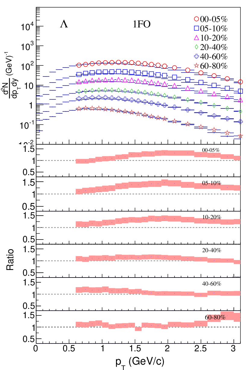
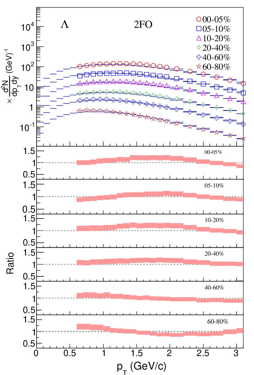


The model spectra in 1FO and 2FO and their comparison with data are shown for the cases of , , , , , , and in Figs. 3, 4, 5, 6, 7, 8 and 9. In 2FO, we find that the agreement between data and model for all the centralities with range upto 2 GeV/c is within for all the hadrons except the multi-strange baryons and resonance. In Figs. 3 and 5, we see that in 1FO, there is a strong tension between the model spectra of and for low and high : in low (high) the model underpredicts (overpredicts) in case of while for , the behaviour is just the reverse of . In 2FO, this tension is reduced considerably. This is the main source of improvement in the fits between 1FO and 2FO. However, the tension does not go away completely in 2FO. There is a clear hint that the model still underpredicts at low , particularly for the most central and peripheral collisions. A similar exercise within the NFO scheme gives a better description of the low pions [24]. It is interesting to note that the value of the light quark nonequilibrium phase space parameter obtained from fit to yield data results in pion chemical potential which is close to pion mass. This could suggest formation of pion condensation [24]. However, within the equilibrium chemical freezeout scenario, this could be interpreted as an indication for further substructure in freezeout and and freezeout separately. There could be also an alternate explanation. The decay of heavier resonances mainly contribute to low . Thus, a deficit in low could also mean that currently the model does not include all the heavier resonances, hinting at the presence of yet unobserved resonances [37]. The spectra of and which freezeout together in 2FO are shown in Figs. 4 and 6. The agreement between model and data is better compared to and . This is also clear from Fig. 1 (c) where we see that in 2FO, except for the centrality bin numbers 1 and 6, for all the other centralities, . The spectra of the multi-strange baryons is shown in Fig. 7. In case of the (), the agreement between data and model for upto 1.5 (2.0) GeV/c is within for all centralities except the most peripheral one. Moreover, 1FO seems to give a better description in the first two centrality bins over the entire range. Within the multiple freezeout scenario, better model description of the spectra plots of the multi-strange hadrons is possible by allowing them to undergo an earlier freezeout compared to and . Here we would like to note that the NFO scheme fails to describe the spectra of all strange baryons. It is only after invoking an early freezeout of the strange baryons that the NFO scheme manages to describe the spectra of the strange baryons [24]. However, it is important to note that within the NFO picture, even after the freezeout of the strange baryons and could still interact and produce . It would be interesting to check whether including the effects of yet unobserved strange hadrons which are predicted by quark models and indicated in lattice QCD simulations improve the agreement between data and model of the spectra of the multi-strange baryons [37].
In case of the resonances, both 1FO and 2FO provide good description of the spectra of which has zero net strangeness while for they fail. In the latter case the lifetime of which is about 4 fm is of the same order as that of the fireball lifetime and hence effects like rescattering and regeneration modify the yield and also the spectra considerably. Previous comparison of the yield between models based on thermal production and data showed that the above medium effects are stronger for central collisions as compared to peripheral ones [36]. Here also we find that the description of the spectra improves as we go to more peripheral cases. In this regard it is to be noted that the lifetime of is an order of magnitude greater than that of and hence we manage to describe its yield and spectra well without incorporating the medium effects of rescattering and regeneration.

We close this section with a short discussion on the minimum number of free parameters required for a good description of the spectra data within the 2FO scheme. So far we have presented results for the most general case treating the thermal () as well as the geometric parameters ( and ) for both the strange and non-strange freezeout surfaces as free parameters. Thus, we have used six free parameters. A closer look at the values of the extracted parameters as given in Table 1 reveals interesting trends. We find the ratio of the geometric parameters of the fireball to be invariant under expansion from the strange to the non-strange FO surface
| (10) |
Thus very good description of the spectra data with similar is obtained with just five parameters using Eq. 10 to fix . Further, we also note that except for the most peripheral centralities of and , the ratio of and is a constant across centralities. Thus the condition of along with Eq. 10 allows for a good 4 parameter (offcourse in order to determine the ratio , atleast one central bin needs to be fitted with five parameters) fit of the spectra data for the centralities data. In Fig. 10, we have compared the for different centralities in the 2FO framework with these different fitting schemes. The most general six parameter fit has been compared with the five parameter fit for all centralities and we find similar goodness of fit. Finally for the centralities, we have also shown the results from the four parameter fit which also yields a similar . The corresponding 1FO values are also shown for comparison.
IV Summary

We have obtained the spectra of , , , , , , and within two schemes of freezeout: 1FO and 2FO. Overall, the description of the spectra improves considerably in 2FO as compared to 1FO with a reduction in by around . The extracted values of the parameters for the strange and non-strange FHs show interesting correlations: for all centralities and for centralities. These conditions allow us to reduce the number of free parameters from six, in case of the most general 2FO scenario, to four with similar . The FHs as obtained in the 1FO and 2FO schemes for the most central bin is plotted in Fig. 11. A clear separation between the non-strange and strange FHs is visible with an earlier freezeout of the hadrons with non-zero strangeness content. As expected from the fitted values of , and , the 1FO hypersurface lies in between the non strange and strange FHs of 2FO. There are some indications of further substructures in the simple 2FO scheme that we have studied here. These are: (a) tension between the model spectra and data of and and (b) overprediction of the spectra in the case of multi-strange baryons. These could be hints of separate freezeout of and and early freezeout of the multi-strange baryons. However, before drawing any conclusion on the nature of freezeout based on these observations, it will be important to account for the contribution to the hadron spectra from the heavier resonances which are yet unobserved but predicted by quark models and hinted upon by LQCD results. Thus, while the current work based on 2FO with an early freezeout of the hadrons with non-zero strangeness content show considerable improvement over the conventional 1FO scheme in describing the data on transverse momentum spectra across all centralities, there are suggestions of possible further substructures in freezeout which are yet to be confirmed.
V Acknowledgement
SC acknowledges discussions and collaborations on freezeout with Rohini Godbole and Sourendu Gupta and thanks “Centre for Nuclear Theory” [PIC XII-RD-VEC-5.02.0500], Variable Energy Cyclotron Centre for support. BM and RS acknowledges financial support from DST SwarnaJayanti and DAE-SRC projects of BM.
References
- [1] S. Borsanyi, Z. Fodor, S. Katz, S. Krieg, C. Ratti, et al., Phys. Rev. Lett. 113, 052301 (2014).
- [2] P. Alba, W. Alberico, R. Bellwied, M. Bluhm, V. Mantovani Sarti, et al., Phys. Lett. B738, 305 (2014).
- [3] A. Bazavov, H. Ding, P. Hegde, O. Kaczmarek, F. Karsch, et al., Phys. Rev. Lett. 109, 192302 (2012).
- [4] P. Braun-Munzinger, J. Stachel, J. Wessels, and N. Xu, Phys. Lett. B365, 1 (1996).
- [5] G. D. Yen and M. I. Gorenstein, Phys. Rev. C59, 2788 (1999).
- [6] F. Becattini, J. Cleymans, A. Keranen, E. Suhonen, and K. Redlich, Phys. Rev. C64, 024901 (2001).
- [7] A. Andronic, P. Braun-Munzinger, and J. Stachel, Nucl. Phys. A772, 167 (2006).
- [8] J. Letessier, J. Rafelski, and A. Tounsi, Phys. Lett. B328, 499 (1994).
- [9] T. Csorgo and L. Csernai, Phys. Lett. B333, 494 (1994).
- [10] L. Csernai and I. Mishustin, Phys. Rev. Lett. 74, 5005 (1995).
- [11] E. Schnedermann, J. Sollfrank, and U. W. Heinz, Phys. Rev. C48, 2462 (1993).
- [12] S. Afanasiev, T. Anticic, B. Baatar, D. Barna, J. Bartke, et al., Nucl. Phys. A715, 161 (2003).
- [13] J. Burward-Hoy (PHENIX Collaboration), Nucl. Phys. A715, 498 (2003).
- [14] W. Broniowski and W. Florkowski, Phys. Rev. Lett. 87, 272302 (2001).
- [15] W. Broniowski and W. Florkowski, Phys. Rev. C65, 064905 (2002).
- [16] M. Rybczynski, W. Florkowski, and W. Broniowski, Phys. Rev. C85, 054907 (2012).
- [17] J. Stachel, A. Andronic, P. Braun-Munzinger, and K. Redlich, J. Phys. Conf. Ser. 509, 012019 (2014).
- [18] J. Steinheimer, J. Aichelin, and M. Bleicher, Phys. Rev. Lett. 110, 042501 (2013).
- [19] F. Becattini, M. Bleicher, T. Kollegger, T. Schuster, J. Steinheimer, et al., Phys. Rev. Lett. 111, 082302 (2013).
- [20] F. Becattini, M. Bleicher, T. Kollegger, M. Mitrovski, T. Schuster, et al., Phys. Rev. C85, 044921 (2012).
- [21] F. Becattini, E. Grossi, M. Bleicher, J. Steinheimer, and R. Stock, (2014), arXiv:1405.0710 [nucl-th] .
- [22] M. Petran, J. Letessier, V. Petracek, and J. Rafelski, Phys. Rev. C88, 034907 (2013).
- [23] V. Begun, W. Florkowski, and M. Rybczynski, Phys. Rev. C90, 014906 (2014a).
- [24] V. Begun, W. Florkowski, and M. Rybczynski, (2014b), arXiv:1405.7252 [hep-ph] .
- [25] S. Chatterjee, R. Godbole, and S. Gupta, Phys. Lett. B727, 554 (2013).
- [26] K. Bugaev, D. Oliinychenko, J. Cleymans, A. Ivanytskyi, I. Mishustin, et al., Europhys. Lett. 104, 22002 (2013).
- [27] S. Chatterjee and B. Mohanty, Phys. Rev. C90, 034908 (2014).
- [28] A. Andronic, P. Braun-Munzinger, J. Stachel, and H. Stocker, Phys. Lett. B697, 203 (2011).
- [29] J. Cleymans, S. Kabana, I. Kraus, H. Oeschler, K. Redlich, et al., Phys. Rev. C84, 054916 (2011).
- [30] A. Kisiel, T. Taluc, W. Broniowski, and W. Florkowski, Comput. Phys. Commun. 174, 669 (2006).
- [31] M. Chojnacki, A. Kisiel, W. Florkowski, and W. Broniowski, Comput. Phys. Commun. 183, 746 (2012).
- [32] W. Broniowski, A. Baran, and W. Florkowski, AIP Conf. Proc. 660, 185 (2003).
- [33] B. Abelev et al. (ALICE Collaboration), Phys. Rev. C88, 044910 (2013a).
- [34] B. B. Abelev et al. (ALICE Collaboration), Phys. Rev. Lett. 111, 222301 (2013b).
- [35] B. B. Abelev et al. (ALICE Collaboration), Phys. Lett. B728, 216 (2014a).
- [36] B. B. Abelev et al. (ALICE Collaboration), (2014b), arXiv:1404.0495 [nucl-ex] .
- [37] A. Bazavov, H. T. Ding, P. Hegde, O. Kaczmarek, F. Karsch, et al., (2014), arXiv:1404.6511 [hep-lat] .