The edit distance for Reeb graphs of surfaces

B. Di Fabio Address: Dipartimento di Matematica, Università di Bologna, P.zza di Porta S. Donato 5, I-

40126

Bologna, Italia
ARCES, Università di Bologna, via Toffano

2/2

, I-

40125

Bologna, Italia Email address: barbara.difabio@unibo.it and C. Landi Address: Dipartimento di Scienze e Metodi dell’Ingegneria, Università di Modena e Reggio Emilia, Via Amendola 2, Pad. Morselli, I-42100 Reggio Emilia, Italia
ARCES, Università di Bologna, via Toffano

2/2

, I-

40125

Bologna, Italia Email address: claudia.landi@unimore.it

Abstract.

Reeb graphs are structural descriptors that capture shape properties of a topological space from the perspective of a chosen function. In this work we define a combinatorial metric for Reeb graphs of orientable surfaces in terms of the cost necessary to transform one graph into another by edit operations. The main contributions of this paper are the stability property and the optimality of this edit distance. More precisely, the stability result states that changes in the functions, measured by the maximum norm, imply not greater changes in the corresponding Reeb graphs, measured by the edit distance. The optimality result states that our edit distance discriminates Reeb graphs better than any other metric for Reeb graphs of surfaces satisfying the stability property.

Key words and phrases:

shape similarity, graph edit distance, Morse function, natural stratification

2010 Mathematics Subject Classification

Primary 05C10, 68T10; Secondary 54C30

Introduction

In shape comparison, a widely used scheme is to measure the dissimilarity between descriptors associated with each shape rather than to match shapes directly. Reeb graphs describe shapes from topological and geometrical perspectives. In this framework, a shape is modeled as a topological space $X$ endowed with a scalar function $f:X\to\mathbb{R}$ . The role of $f$ is to explore geometrical properties of the space $X$ . The Reeb graph of $f$ is obtained by shrinking each connected component of a level set of $f$ to a single point [20]. Reeb graphs have been used as an effective tool for shape analysis and description tasks since [24, 23].

One of the most important questions is whether Reeb graphs are robust against perturbations that may occur because of noise and approximation errors in the data acquisition process. Whereas in the past researchers dealt with this problem developing heuristics so that Reeb graphs would be resistant to connectivity changes caused by simplification, subdivision and remesh, and robust against noise and certain changes due to deformation [11, 2], in the last years the question of Reeb graph stability has been investigated from the theoretical point of view. In [7] an edit distance between Reeb graphs of curves endowed with Morse functions is introduced and shown to yield stability. Importantly, despite the combinatorial nature of this distance, it coincides with the natural pseudo-distance between shapes [8], thus showing the maximal discriminative power for this sort of distances. Very recently a functional distortion distance between Reeb graphs has been proposed in [1], with proven stable and discriminative properties. The functional distortion distance is based on continuous maps between the topological spaces realizing the Reeb graphs, so that it is not combinatorial in its definition. Noticeably, it allows for comparison of non-homeomorphic spaces meaning that it can be used to deal also with artifacts that change the homotopy type of the space, although as a consequence it cannot fully discriminate shapes and stability is not proven in that case.

In this paper we deal with the comparison problem for Reeb graphs of surfaces. Indeed the case of surfaces seems to us the most interesting area of application of the Reeb graph as a shape descriptor. As a tradeoff between generality and simplicity, we confine ourselves to the case of smooth compact orientable surfaces without boundary endowed with simple Morse functions.

The basic properties we consider important for a metric between Reeb graphs are: the robustness to perturbations of the input functions; the ability to discriminate functions on the same manifold; the deployment of the combinatorial nature of graphs. For this reason, we apply to the case of surfaces the same underlying ideas as used in [7] for curves. Starting from Reeb graphs labeled on the vertices by the function values, the following steps are carried out: first, a set of admissible edit operations is detected to transform a labeled Reeb graph into another; then a suitable cost is associated to each edit operation; finally, a combinatorial dissimilarity measure between labeled Reeb graphs, called an edit distance, is defined in terms of the least cost necessary to transform one graph into another by edit operations. However, the passage from curves to surfaces is not automatic since Reeb graphs of surfaces are structurally different from those of curves. For example, the degree of vertices is different for Reeb graphs of curves and surfaces. Therefore, the set of edit operations as well as their costs cannot be directly imported from the case of curves but need to be suitably defined. In conclusion, our edit distance between Reeb graphs belongs to the family of Graph Edit Distances [10], widely used in pattern analysis.

Our first main result is that changes in the functions, measured by the maximum norm, imply not greater changes in this edit distance, yielding the stability property under function perturbations. To prove this result, we track the changes in the Reeb graphs as the function varies along a linear path avoiding degeneracies. From the stability property, we deduce that the edit distance between the Reeb graphs of two functions $f$ and $g$ defined on a surface is a lower bound for the natural pseudo-distance between $f$ and $g$ obtained by minimizing the change in the functions due to the application of a self-diffeomorphism of the manifold, with respect to the maximum norm. The natural pseudo-distance can be thought as a way to compare $f$ and $g$ directly, while the edit distance provides an indirect comparison between $f$ and $g$ through their Reeb graphs. Thus, by virtue of the stability result, the edit distance provides a combinatorial tool to estimate the natural pseudo-distance.

Our second contribution is the proof that the edit distance between Reeb graphs of surfaces actually coincides with the natural pseudo-distance. This is proved by showing that for every edit operation on a Reeb graph there is a self-homeomorphism of the surface whose cost is not greater than that of the considered edit operation. This result implies that the edit distance is actually a metric and not only a pseudo-metric. Morever it shows that the edit distance is an optimal distance for Reeb graphs of surfaces in that it has the maximum discriminative power among all the distances between Reeb graphs of surfaces with the stability property.

In conclusion, this paper shows that the results of [7] for curves also hold in the more interesting case of surfaces.

The paper is organized as follows. In Section 1 we recall the basic properties of labeled Reeb graphs of orientable surfaces. In Section 2 we define the edit deformations between labeled Reeb graphs, and show that through a finite sequence of these deformations we can always transform a Reeb graph into another. In Section 3 we define the cost associated with each type of edit deformation and the edit distance in terms of this cost. Section 4 illustrates the robustness of Reeb graphs with respect to the edit distance. Eventually, Section 5 provides relationships between our edit distance and other stable metrics: the natural pseudo-distance, the bottleneck distance and the functional distortion distance.

A number of questions remain open and are not treated in this paper. The most important one is how to compute the edit distance. Indeed, whereas in some particular cases we can deduce the value of the edit distance from the lower bounds provided by the bottleneck distance of persistence diagrams or the functional distortion distance of Reeb graphs, in general we do not know how to compute it. A second open problem is to which extent the theory developed in this paper for the smooth category can be transported into the piecewise linear category. A third question that would deserve investigation is how to generalize the edit distance to compare functions on non-homeomorphic surfaces as well, and the relationship with the functional distortion distance in that case.

1. Labeled Reeb graphs of orientable surfaces

Hereafter, ${\mathcal{M}}$ denotes a connected, closed (i.e. compact and without boundary), orientable, smooth surface of genus $\mathfrak{g}$ , and $\mathcal{F}({\mathcal{M}})$ the set of $C^{\infty}$ real functions on ${\mathcal{M}}$ .

For $f\in\mathcal{F}({\mathcal{M}})$ , we denote by $K_{f}$ the set of its critical points. If $p\in K_{f}$ , then the real number $f(p)$ is called a critical value of $f$ , and the set $\{q\in{\mathcal{M}}:q\in f^{-1}(f(p))\}$ is called a critical level of $f$ . Moreover, a critical point $p$ is called non-degenerate if the Hessian matrix of $f$ at $p$ is non-singular. The index of a non-degenerate critical point $p$ of $f$ is the dimension of the largest subspace of the tangent space to ${\mathcal{M}}$ at $p$ on which the Hessian matrix is negative definite. In particular, the index of a point $p\in K_{f}$ is equal to 0,1, or 2 depending on whether $p$ is a minimum, a saddle, or a maximum point of $f$ .

A function $f\in\mathcal{F}({\mathcal{M}})$ is called a Morse function if all its critical points are non-degenerate. Besides, a Morse function is said to be simple if each critical level contains exactly one critical point. The set of simple Morse functions will be denoted by $\mathcal{F}^{0}({\mathcal{M}})$ , as a reminder that it is a sub-manifold of $\mathcal{F}({\mathcal{M}})$ of co-dimension 0 (see also Section 4).

Definition 1.1.

Let $f\in\mathcal{F}^{0}({\mathcal{M}})$ , and define on ${\mathcal{M}}$ the following equivalence relation: for every $p,q\in{\mathcal{M}}$ , $p\sim_{f}q$ whenever $p,q$ belong to the same connected component of $f^{-1}(f(p))$ . The quotient space ${\mathcal{M}}/\sim_{f}$ is the Reeb graph associated with $f$ .

Our assumption that $f$ is a simple Morse function allows us to consider the space ${\mathcal{M}}/\sim_{f}$ as a graph whose vertices correspond bijectively to the critical points of $f$ . For this reason, in the following, we will often identify vertices with the corresponding critical points.

Proposition 1.2.

([20]) The Reeb graph $\Gamma_{f}$ associated with $f\in\mathcal{F}^{0}({\mathcal{M}})$ is a finite and connected simplicial complex of dimension 1. A vertex of $\Gamma_{f}$ has degree equal to 1 if it corresponds to a critical point of $f$ of index 0 or 2, while it has degree equal to 2,3, or 4 if it corresponds to a critical point of $f$ of index 1.

Throughout this paper, Reeb graphs are regarded as combinatorial graphs and not as topological spaces. The vertex set of $\Gamma_{f}$ will be denoted by $V(\Gamma_{f})$ , and its edge set by $E(\Gamma_{f})$ . Moreover, if $v_{1},v_{2}\in V(\Gamma_{f})$ are adjacent vertices, i.e., connected by an edge, we will write $e(v_{1},v_{2})\in E(\Gamma_{f})$ .

Our assumptions that ${\mathcal{M}}$ is orientable, compact and without boundary ensure that there are no vertices of degree 2 or 4. Moreover, if $p,q,r$ denote the number of minima, maxima, and saddle points of $f$ , from the relationships between the Euler characteristic of ${\mathcal{M}}$ , $\chi({\mathcal{M}})$ , and $p,q,r$ , i.e. $\chi({\mathcal{M}})=p+q-r$ , and between $\chi({\mathcal{M}})$ and the genus $\mathfrak{g}$ of ${\mathcal{M}}$ , i.e. $\chi({\mathcal{M}})=2-2\mathfrak{g}$ , it follows that the cardinality of $V(\Gamma_{f})$ , which is $p+q+r$ , is also equal to $2(p+q+\mathfrak{g}-1)$ , i.e. is even in number. The minimum number of vertices of a Reeb graph is achieved whenever $p=q=1$ , and consequently $r=2\mathfrak{g}$ . In this case the cardinality of $V(\Gamma_{f})$ is equal to $2\mathfrak{g}+2$ . In general, if ${\mathcal{M}}$ has genus $\mathfrak{g}$ then $\Gamma_{f}$ has exactly $\mathfrak{g}$ linearly independent cycles. We will call a cycle of length $m$ in the graph an $m$ -cycle. These observations motivate the following definition.

Definition 1.3.

We shall call minimal the Reeb graph $\Gamma_{f}$ of a function $f$ having $p=q=1$ . Moreover, we say that $\Gamma_{f}$ is canonical if it is minimal and all its cycles, if any, are 2-cycles.

We underline that our definition of canonical Reeb graph is slightly different from the one in [13]. This choice has been done to simplify the proof of Proposition 2.7.

Examples of minimal and canonical Reeb graphs are displayed in Figure 1.

Refer to caption — Figure 1. Examples of minimal Reeb graphs. The graph on the right is also canonical.

In what follows, we label the vertices of $\Gamma_{f}$ by equipping each of them with the value of $f$ at the corresponding critical point. We denote such a labeled graph by $(\Gamma_{f},\ell_{f})$ , where $\ell_{f}:V(\Gamma_{f})\to\mathbb{R}$ is the restriction of $f:{\mathcal{M}}\to\mathbb{R}$ to $K_{f}$ . In a labeled Reeb graph, each vertex $v$ of degree 3 has at least two of its adjacent vertices, say $v_{1},v_{2}$ , such that $\ell_{f}(v_{1})<\ell_{f}(v)<\ell_{f}(v_{2})$ . An example is displayed in Figure 2.

Let us consider the realization problem, i.e. the problem of constructing a smooth surface and a simple Morse function on it from a graph on an even number of vertices, all of which are of degree 1 or 3, appropriately labeled. We need the following definition.

Definition 1.4.

We shall say that two labeled Reeb graphs $(\Gamma_{f},\ell_{f}),(\Gamma_{g},\ell_{g})$ are isomorphic, and we write $(\Gamma_{f},\ell_{f})\cong(\Gamma_{g},\ell_{g})$ , if there exists a graph isomorphism $\Phi:V(\Gamma_{f})\rightarrow V(\Gamma_{g})$ such that, for every $v\in V(\Gamma_{f})$ , $\ell_{f}(v)=\ell_{g}(\Phi(v))$ (i.e. $\Phi$ preserves edges and vertex labels).

Proposition 1.5 (Realization Theorem).

Let $(\Gamma,\ell)$ be a labeled graph, where $\Gamma$ is a graph with $m$ linearly independent cycles, on an even number of vertices, all of which are of degree 1 or 3, and $\ell:V(\Gamma)\rightarrow\mathbb{R}$ is an injective function such that, for any vertex $v$ of degree 3, at least two among its adjacent vertices, say $w,w^{\prime}$ , are such that $\ell(w)<\ell(v)<\ell(w^{\prime})$ . Then an orientable closed surface ${\mathcal{M}}$ of genus $\mathfrak{g}=m$ , and a simple Morse function $f:{\mathcal{M}}\to\mathbb{R}$ exist such that $(\Gamma_{f},\ell_{f})\cong(\Gamma,\ell)$ .

Proof.

Under our assumption on the degree of vertices of $\Gamma$ , ${\mathcal{M}}$ and $f$ can be constructed as in the proof of Thm. 2.1 in [17]. ∎

We now deal with the uniqueness problem, up to isomorphism of labeled Reeb graphs. First of all we consider the following two equivalence relations on $\mathcal{F}^{0}({\mathcal{M}})$ .

Definition 1.6.

Let $\mathcal{D}({\mathcal{M}})$ be the set of self-diffeomorphisms of ${\mathcal{M}}$ . Two functions $f,g\in\mathcal{F}^{0}({\mathcal{M}})$ are called right-equivalent (briefly, $R$ -equivalent) if there exists $\xi\in\mathcal{D}({\mathcal{M}})$ such that $f=g\circ\xi$ . Moreover, $f,g$ are called right-left equivalent (briefly, RL-equivalent) if there exist $\xi\in\mathcal{D}({\mathcal{M}})$ and an orientation preserving self-diffeomorphism $\eta$ of $\mathbb{R}$ such that $f=\eta\circ g\circ\xi$ .

These equivalence relations on functions are mirrored by Reeb graphs isomorphisms.

Proposition 1.7 (Uniqueness Theorem).

If $f,g\in\mathcal{F}^{0}({\mathcal{M}})$ , then

(1)

$f$ and $g$ are RL-equivalent if and only if their Reeb graphs $\Gamma_{f}$ and $\Gamma_{g}$ are isomorphic by an isomorphism $\Phi:V(\Gamma_{f})\to V(\Gamma_{g})$ that preserves the vertex order, i.e., for every $v,w\in V(\Gamma_{f})$ , $\ell_{f}(v)<\ell_{f}(w)$ if and only if $\ell_{g}(\Phi(v))<\ell_{g}(\Phi(w))$ ;
(2)

$f$ and $g$ are $R$ -equivalent if and only if their labeled Reeb graphs $(\Gamma_{f},\ell_{f})$ and $(\Gamma_{g},\ell_{g})$ are isomorphic.

Proof.

For the proof of statement (1) see [15, 22]. As for statement (2), we note that two $R$ -equivalent functions are, in particular, $RL$ -equivalent. Hence, by statement (1), their Reeb graphs are isomorphic by an isomorphism that preserves the vertex order. Since $f$ and $g$ necessarily have the same critical values, this isomorphism also preserves labels. Vice-versa, if $(\Gamma_{f},\ell_{f})$ and $(\Gamma_{g},\ell_{g})$ are isomorphic, then $f$ and $g$ have the same critical values. Moreover, by statement (1), there exist $\xi\in\mathcal{D}({\mathcal{M}})$ and an orientation preserving self-diffeomorphism $\eta$ of $\mathbb{R}$ such that $f=\eta\circ g\circ\xi$ . Let us set $h=g\circ\xi$ . The function $h$ belongs to $\mathcal{F}^{0}({\mathcal{M}})$ and has the same critical points with the same indexes as $f$ , and the same critical values as $g$ and hence as $f$ . Thus, we can apply [14, Lemma 1] to $f$ and $h$ and deduce the existence of a self-diffeomorphism $\xi^{\prime}$ of ${\mathcal{M}}$ such that $f=h\circ\xi^{\prime}$ . Thus $f=g\circ\xi\circ\xi^{\prime}$ , yielding that $f$ and $g$ are $R$ -equivalent. A direct proof of the $R$ -equivalence of functions with isomorphic labeled Reeb graphs is also obtainable from Lemma 5.3. ∎

2. edit deformations between labeled Reeb graphs

In this section we list the edit deformations admissible to transform labeled Reeb graphs into one another when different simple Morse functions on the same surface are considered. We introduce at first elementary deformations, then, by virtue of the Realization Theorem (Proposition 1.5), the deformations obtained by their composition.

Elementary deformations allow us to insert or delete a vertex of degree 1 together with an adjacent vertex of degree 3 (deformations of birth type (B) and death type (D)), maintain the same vertices and edges while changing the vertex labels (deformations of relabeling type (R)), or change some vertices adjacencies and labels (deformations of type (K₁), (K₂), (K₃) introduced by Kudryavtseva in [13]). A sketch of these elementary deformations can be found in Table 1. The formal definition is as follows.

Definition 2.1.

With the convention of denoting the open interval with endpoints $a,b\in\mathbb{R}$ by $]a,b[$ , the elementary deformations of type (B), (D), (R), (K_i), $i=1,2,3$ , are defined as follows.

(B)
$T$ is an elementary deformation of $(\Gamma_{f},\ell_{f})$ of type (B) if, for a fixed edge $e(v_{1},v_{2})\in E(\Gamma_{f})$ , with $\ell_{f}(v_{1})<\ell_{f}(v_{2})$ , $T(\Gamma_{f},\ell_{f})$ is a labeled graph $(\Gamma,\ell)$ such that
- –
  
  $V(\Gamma)=V(\Gamma_{f})\cup\{u_{1},u_{2}\}$ ;
- –
  
  $E(\Gamma)=\left(E(\Gamma_{f})-\{e(v_{1},v_{2})\}\right)\cup\{e(v_{1},u_{1}),e(u_{1},u_{2}),e(u_{1},v_{2})\}$ ;
- –
  
  ${\ell}_{|V(\Gamma_{f})}=\ell_{f}$ and $\ell_{f}(v_{1})<\ell(u_{i})<\ell(u_{j})<\ell_{f}(v_{2})$ , with $\ell^{-1}(]\ell(u_{i}),\ell(u_{j})[)=\emptyset$ , $i,j\in\{1,2\},i\neq j$ .
(D)
$T$ is an elementary deformation of $(\Gamma_{f},\ell_{f})$ of type (D) if, for fixed edges $e(v_{1},u_{1})$ , $e(u_{1},u_{2})$ , $e(u_{1},v_{2})\in E(\Gamma_{f})$ , $u_{2}$ being of degree 1, such that $\ell_{f}(v_{1})<\ell_{f}(u_{i})<\ell_{f}(u_{j})<\ell_{f}(v_{2})$ , with $\ell_{f}^{-1}(]\ell_{f}(u_{i}),\ell_{f}(u_{j})[)=\emptyset$ , $i,j\in\{1,2\},i\neq j$ , $T(\Gamma_{f},\ell_{f})$ is a labeled graph $(\Gamma,\ell)$ such that
- –
  
  $V(\Gamma)=V(\Gamma_{f})-\{u_{1},u_{2}\}$ ;
- –
  
  $E(\Gamma)=\left(E(\Gamma_{f})-\{e(v_{1},u_{1}),e(u_{1},u_{2}),e(u_{1},v_{2})\}\right)\cup\{e(v_{1},v_{2})\}$ ;
- –
  
  $\ell={\ell_{f}}_{|V(\Gamma_{f})-\{u_{1},u_{2}\}}$ .
(R)
$T$ is an elementary deformation of $(\Gamma_{f},\ell_{f})$ of type (R) if $T(\Gamma_{f},\ell_{f})$ is a labeled graph $(\Gamma,\ell)$ such that
- –
  
  $\Gamma=\Gamma_{f}$ ;
- –
  
  $\ell:V(\Gamma)\to\mathbb{R}$ induces the same vertex-order as $\ell_{f}$ except for at most two non-adjacent vertices, say $u_{1},u_{2}$ , with $\ell_{f}(u_{1})<\ell_{f}(u_{2})$ and $\ell_{f}^{-1}(]\ell_{f}(u_{1}),\ell_{f}(u_{2})[)=\emptyset$ , for which $\ell(u_{1})>\ell(u_{2})$ and $\ell^{-1}(]\ell(u_{2}),\ell(u_{1})[)=\emptyset$ .
(K₁)
$T$ is an elementary deformation of $(\Gamma_{f},\ell_{f})$ of type (K₁) if, for fixed edges $e(v_{1},u_{1})$ , $e(u_{1},u_{2})$ , $e(u_{1},v_{4})$ , $e(u_{2},v_{2})$ , $e(u_{2},v_{3})\in E(\Gamma_{f})$ , with two among $v_{2},v_{3},v_{4}$ possibly coincident, $\ell_{f}(v_{1})<\ell_{f}(u_{1})<\ell_{f}(u_{2})<\ell_{f}(v_{2}),\ell_{f}(v_{3})$ , $\ell_{f}(v_{4})$ , and $\ell_{f}^{-1}(]\ell_{f}(u_{1}),\ell_{f}(u_{2})[)=\emptyset$ (resp. $\ell_{f}(v_{2})$ , $\ell_{f}(v_{3})$ , $\ell_{f}(v_{4})<\ell_{f}(u_{2})<\ell_{f}(u_{1})$ $<\ell_{f}(v_{1})$ , and $\ell_{f}^{-1}(]\ell_{f}(u_{2}),\ell_{f}(u_{1})[)=\emptyset$ ), $T(\Gamma_{f},\ell_{f})$ is a labeled graph $(\Gamma,\ell)$ such that:
- –
  
  $V(\Gamma)=V(\Gamma_{f})$ ;
- –
  
  $E(\Gamma)=\left(E(\Gamma_{f})-\{e(v_{1},u_{1}),e(u_{2},v_{2})\}\right)\cup\{e(v_{1},u_{2}),e(u_{1},v_{2})\}$ ;
- –
  
  ${\ell}_{|V(\Gamma)-\{u_{1},u_{2}\}}=\ell_{f}$ and $\ell_{f}(v_{1})<\ell(u_{2})<\ell(u_{1})<\ell_{f}(v_{2})$ , $\ell_{f}(v_{3})$ , $\ell_{f}(v_{4})$ , with $\ell^{-1}(]\ell(u_{2}),\ell(u_{1})[)$ $=\emptyset$ (resp. $\ell_{f}(v_{2})$ , $\ell_{f}(v_{3})$ , $\ell_{f}(v_{4})<\ell(u_{1})<\ell(u_{2})<\ell_{f}(v_{1})$ , with $\ell^{-1}(]\ell(u_{1}),\ell(u_{2})[)=\emptyset$ ).
(K₂)
$T$ is an elementary deformation of $(\Gamma_{f},\ell_{f})$ of type (K₂) if, for fixed edges $e(v_{1},u_{1})$ , $e(v_{2},u_{1})$ , $e(u_{1},u_{2})$ , $e(u_{2},v_{3})$ , $e(u_{2},v_{4})\in E(\Gamma_{f})$ , with $u_{1},u_{2}$ of degree 3, $v_{2},v_{3}$ possibly coincident with $v_{1},v_{4}$ , respectively, and $\ell_{f}(v_{1}),\ell_{f}(v_{2})$ $<\ell_{f}(u_{1})<\ell_{f}(u_{2})<\ell_{f}(v_{3}),\ell_{f}(v_{4})$ , with $\ell_{f}^{-1}(]\ell_{f}(u_{1}),\ell_{f}(u_{2})[)=\emptyset$ , $T(\Gamma_{f},\ell_{f})$ is a labeled graph $(\Gamma,\ell)$ such that:
- –
  
  $V(\Gamma)=V(\Gamma_{f})$ ;
- –
  
  $E(\Gamma)=\left(E(\Gamma_{f})-\{e(v_{1},u_{1}),e(u_{2},v_{3})\}\right)\cup\{e(v_{1},u_{2}),e(u_{1},v_{3})\}$ ;
- –
  
  ${\ell}_{|V(\Gamma)-\{u_{1},u_{2}\}}=\ell_{f}$ and $\ell_{f}(v_{1})$ , $\ell_{f}(v_{2})<\ell(u_{2})<\ell(u_{1})<\ell_{f}(v_{3})$ , $\ell_{f}(v_{4})$ , with $\ell^{-1}(]\ell(u_{2}),\ell(u_{1})[)=\emptyset$ .
(K₃)
$T$ is an elementary deformation of $(\Gamma_{f},\ell_{f})$ of type (K₃) if, for fixed edges $e(v_{1},u_{2})$ , $e(u_{1},u_{2})$ , $e(v_{2},u_{1})$ , $e(u_{1},v_{3})$ , $e(u_{2},v_{4})\in E(\Gamma_{f})$ , with $u_{1},u_{2}$ of degree 3, $v_{2},v_{3}$ possibly coincident with $v_{1},v_{4}$ , respectively, and $\ell_{f}(v_{1}),\ell_{f}(v_{2})<\ell_{f}(u_{2})<\ell_{f}(u_{1})<\ell_{f}(v_{3}),\ell_{f}(v_{4})$ , with $\ell_{f}^{-1}(]\ell_{f}(u_{2}),\ell_{f}(u_{1})[)=\emptyset$ , $T(\Gamma_{f},\ell_{f})$ is a labeled graph $(\Gamma,\ell)$ such that:
- –
  
  $V(\Gamma)=V(\Gamma_{f})$ ;
- –
  
  $E(\Gamma)=\left(E(\Gamma_{f})-\{e(v_{1},u_{2}),e(u_{1},v_{3})\}\right)\cup\{e(v_{1},u_{1}),e(u_{2},v_{3})\}$ ;
- –
  
  ${\ell}_{|V(\Gamma)-\{u_{1},u_{2}\}}=\ell_{f}$ and $\ell_{f}(v_{1})$ , $\ell_{f}(v_{2})<\ell(u_{1})<\ell(u_{2})<\ell_{f}(v_{3})$ , $\ell_{f}(v_{4})$ , with $\ell^{-1}(]\ell(u_{1}),\ell(u_{2})[)=\emptyset$ .

[Uncaptioned image] — Table 1. A schematization of the elementary deformations of a labeled Reeb graph provided by Definition 2.1.

We underline that the definition of the deformations of type (B), (D) and (R) is essentially different from the definition of analogous deformations in the case of Reeb graphs of curves as given in [7], even if the associated cost will be the same (see Section 3). This is because the degree of the involved vertices is 2 for Reeb graphs of closed curves, whereas it is 1 or 3 for Reeb graphs of surfaces.

Proposition 2.2.

Let $f\in\mathcal{F}^{0}({\mathcal{M}})$ and $(\Gamma,\ell)=T(\Gamma_{f},\ell_{f})$ for some elementary deformation $T$ . Then there exists $g\in\mathcal{F}^{0}({\mathcal{M}})$ such that $(\Gamma_{g},\ell_{g})\cong(\Gamma,\ell)$ .

Proof.

The claim follows from Proposition 1.5. ∎

As a consequence of Proposition 2.2, we can apply elementary deformations iteratively. This fact is used in the next Definition 2.3. Given an elementary deformation $T$ of $(\Gamma_{f},\ell_{f})$ and an elementary deformation $S$ of $T(\Gamma_{f},\ell_{f})$ , the juxtaposition $ST$ means applying first $T$ and then $S$ .

Definition 2.3.

We shall call deformation of $(\Gamma_{f},\ell_{f})$ any finite ordered sequence $T=(T_{1},T_{2},\ldots,T_{r})$ of elementary deformations such that $T_{1}$ is an elementary deformation of $(\Gamma_{f},\ell_{f})$ , $T_{2}$ is an elementary deformation of $T_{1}(\Gamma_{f},\ell_{f})$ , …, $T_{r}$ is an elementary deformation of $T_{r-1}T_{r-2}\cdots T_{1}(\Gamma_{f},\ell_{f})$ . We shall denote by $T(\Gamma_{f},\ell_{f})$ the result of the deformation $T_{r}T_{r-1}\cdots T_{1}$ applied to $(\Gamma_{f},\ell_{f})$ .

In the rest of the paper we write ${\mathcal{T}}((\Gamma_{f},\ell_{f}),(\Gamma_{g},\ell_{g}))$ to denote the set of deformations turning $(\Gamma_{f},\ell_{f})$ into $(\Gamma_{g},\ell_{g})$ up to isomorphism:

{\mathcal{T}}((\Gamma_{f},\ell_{f}),(\Gamma_{g},\ell_{g}))=\{T=(T_{1},\ldots,T_{n}),n\geq 1:T(\Gamma_{f},\ell_{f})\cong(\Gamma_{g},\ell_{g})\}.

We now introduce the concept of inverse deformation.

Definition 2.4.

Let $T\in{\mathcal{T}}((\Gamma_{f},\ell_{f}),(\Gamma_{g},\ell_{g}))$ and let $\Phi$ be the labeled graph isomorphism between $T(\Gamma_{f},\ell_{f})$ and $(\Gamma_{g},\ell_{g})$ . We denote by $T^{-1}$ , and call it the inverse of $T$ in ${\mathcal{T}}((\Gamma_{g},\ell_{g}),(\Gamma_{f},\ell_{f}))$ , the deformation that acts on the vertices, edges, and labels of $(\Gamma_{g},\ell_{g})$ as follows: identifying $T(\Gamma_{f},\ell_{f})$ with $(\Gamma_{g},\ell_{g})$ via $\Phi$ ,

•

if $T$ is an elementary deformation of type (D) deleting two vertices, then $T^{-1}$ is of type (B) inserting the same vertices, with the same labels, and viceversa;
•

if $T$ is an elementary deformation of type (R) relabeling vertices of $V(\Gamma_{f})$ , then $T^{-1}$ is again of type (R) relabeling these vertices in the inverse way;
•

if $T$ is an elementary deformation of type (K₁) relabeling two vertices, then $T^{-1}$ is again of type (K₁) relabeling the same vertices in the inverse way;
•

if $T$ is an elementary deformation of type (K₂) relabeling two vertices, then $T^{-1}$ is of type (K₃) relabeling the same vertices in the inverse way, and viceversa;
•

if $T=(T_{1},\ldots,T_{r})$ , then $T^{-1}=(T^{-1}_{r},\ldots,T^{-1}_{1})$ .

From the fact that $T^{-1}T(\Gamma_{f},\ell_{f})\cong(\Gamma_{f},\ell_{f})$ it follows that the set ${\mathcal{T}}((\Gamma_{f},\ell_{f}),(\Gamma_{g},\ell_{g}))$ , when non-empty, always contains infinitely many deformations. We end the section proving that for $f,g\in\mathcal{F}^{0}({\mathcal{M}})$ it is always non-empty. We first need two lemmas which are widely inspired by [13, Lemma 1 and Thm. 1], respectively.

Lemma 2.5.

Let $(\Gamma_{f},\ell_{f})$ be a labeled Reeb graph. The following statements hold:

$(i)$

For any $u,v\in V(\Gamma_{f})$ corresponding to two minima or two maxima of $f$ , there exists a deformation $T$ such that $u$ and $v$ are adjacent to the same vertex $w$ in $T(\Gamma_{f},\ell_{f})$ .
$(ii)$

For any $m$ -cycle $C$ in $\Gamma_{f}$ , $m\geq 2$ , there exists a deformation $T$ such that $C$ is a 2-cycle in $T(\Gamma_{f},\ell_{f})$ .

Proof.

Let us prove statement $(i)$ assuming that in $(\Gamma_{f},\ell_{f})$ there exist two vertices $u,v$ corresponding to two minima of $f$ . The case of maxima is analogous.

Let us consider a path $\gamma$ on $\Gamma_{f}$ having $u,v$ as endpoints, whose length is $m\geq 2$ , and the finite sequence of vertices through which it passes is $(w_{0},w_{1},\ldots,w_{m})$ , with $w_{0}=u,w_{m}=v$ , and $w_{i}\neq w_{j}$ for $i\neq j$ . We aim at showing that there exists a deformation $T$ such that in $T(\Gamma_{f},\ell_{f})$ the vertices $u,v$ are adjacent to the same vertex $w$ , with $w\in\{w_{1},\dots,w_{m-1}\}$ , and thus the path $\gamma$ is transformed by $T$ into a path $\gamma^{\prime}$ which is of length 2 and passes through the vertices $u,w,v$ .

If $m=2$ , then it is sufficient to take $T$ as the deformation of type (R) such that $T(\Gamma_{f},\ell_{f})=(\Gamma_{f},\ell_{f})$ since $\gamma$ already coincides with $\gamma^{\prime}$ . If $m>2$ , let $w_{i}=\mathrm{argmax}\{\ell_{f}(w_{j}):w_{j}\mbox{ with }0\leq j\leq m\}$ . It holds that $w_{i}\neq u,v$ because $u,v$ are minima of $f$ and is unique because $f$ is simple. It is easy to observe that, in a neighborhood of $w_{i}$ , possibly after a finite sequence of deformations of type (R), the graph gets one of the configurations shown in Figure 3 $(a)-(e)$ (left).

The same figure shows that a finite sequence of deformations of type (K₁), (K₃), and, possibly, (R) transforms the simple path $\gamma$ , which has length $m$ , into a simple path of length $m-1$ . Iterating this procedure, we deduce the desired claim.

The proof of statement $(ii)$ is analogous to that of statement $(i)$ , provided that $\gamma$ is taken to be an $m$ -cycle with $u\equiv v$ of degree 3, and $u=\mathrm{argmin}\{\ell_{f}(w_{j}):w_{j}\mbox{ with }0\leq j\leq m-1\}$ . ∎

Lemma 2.6.

Every labeled Reeb graph $(\Gamma_{f},\ell_{f})$ can be transformed into a canonical one through a finite sequence of elementary deformations.

Proof.

Our proof is in two steps: first we show how to transform an arbitrary Reeb graph into a minimal one; then how to reduce a minimal Reeb graph to the canonical form.

The first step is by induction on $s=p+q$ , with $p$ and $q$ denoting the number of minima and maxima of $f$ . If $s=2$ , then $\Gamma_{f}$ is already minimal (see Definition 1.3). Let us assume that any Reeb graph with $s\geq 2$ vertices of degree 1 can be transformed into a minimal one through a certain deformation. Let $\Gamma_{f}$ have $s+1$ vertices of degree 1. Thus, at least one between $p$ and $q$ is greater than one. Let $p>1$ (the case $q>1$ is analogous). By Lemma 2.5 $(i)$ , if $u,v$ correspond to two minima of $f$ , we can construct a deformation $T$ such that in $T(\Gamma_{f},\ell_{f})$ these vertices are both adjacent to a certain vertex $w$ of degree 3. Let $T(\Gamma_{f},\ell_{f})=(\Gamma,\ell)$ , with $\ell(u)<\ell(v)<\ell(w)$ . If there exists a vertex $w^{\prime}\in\ell^{-1}(]\ell(v),\ell(w)[)$ , since $v,w^{\prime}$ cannot be adjacent, we can apply a deformation of type (R) relabeling only $v$ , and get a new labeling $\ell^{\prime}$ such that $\ell^{\prime}(w^{\prime})$ is not contained in $]\ell^{\prime}(v),\ell^{\prime}(w)[$ . Possibly repeating this procedure finitely many times, we get a new labeling, that for simplicity we still denote by $\ell$ , such that $\ell^{-1}(]\ell(v),\ell(w)[)=\emptyset$ . Hence, through a deformation of type (D) deleting $v,w$ , the resulting labeled Reeb graph has $s$ vertices of degree 1. By the inductive hypothesis, it can be transformed into a minimal Reeb graph.

Now we prove the second step. Let $\Gamma_{f}$ be a minimal Reeb Graph, i.e. $p=q=1$ . The total number of splitting saddles (i.e. vertices of degree 3 for which there are two higher adjacent vertices) of $\Gamma_{f}$ is $\mathfrak{g}$ . If $\mathfrak{g}=0$ , then $\Gamma_{f}$ is already canonical. Let us consider the case $\mathfrak{g}\geq 1$ . Let $v\in V(\Gamma_{f})$ be a splitting saddle such that, for every cycle $C$ containing $v$ , $\ell_{f}(v)=\underset{w\in C}{\min}\{\ell_{f}(w)\}$ , and let $C$ be one of these cycles. By Lemma 2.5 $(ii)$ , there exists a deformation $T$ that transforms $C$ into a 2-cycle, still having $v$ as the lowest vertex. Let $v^{\prime}$ be the highest vertex in this $2$ -cycle. We observe that no other cycles of $T(\Gamma_{f},\ell_{f})$ contain $v$ and $v^{\prime}$ , otherwise the initial assumption on $\ell_{f}(v)$ would be contradicted. Hence $v$ , $v^{\prime}$ and the edges adjacent to them are not touched when applying again Lemma 2.5 $(ii)$ to reduce the length of another cycle. Therefore, iterating the same argument on a different splitting saddle, after at most $\mathfrak{g}$ iterations (actually at most $\mathfrak{g}-1$ would suffice) $\Gamma_{f}$ is transformed into a canonical Reeb graph. ∎

Proposition 2.7.

Let $f,g\in\mathcal{F}^{0}({\mathcal{M}})$ . The set ${\mathcal{T}}((\Gamma_{f},\ell_{f}),(\Gamma_{g},\ell_{g}))$ is non-empty.

Proof.

By Lemma 2.6 we can find two deformations $T_{f}$ and $T_{g}$ transforming $(\Gamma_{f},\ell_{f})$ and $(\Gamma_{g},\ell_{g})$ , respectively, into canonical Reeb graphs. Apart from the labels, $\Gamma_{f}$ and $\Gamma_{g}$ are isomorphic because associated with the same surface ${\mathcal{M}}$ . Hence, $T_{f}(\Gamma_{f},\ell_{f})$ can be transformed into a graph isomorphic to $T_{g}(\Gamma_{g},\ell_{g})$ through an elementary deformation of type (R), say $T_{\mbox{\tiny{R}}}$ . Thus $(\Gamma_{g},\ell_{g})\cong T_{g}^{-1}T_{\mbox{\tiny{R}}}T_{f}(\Gamma_{f},\ell_{f})$ , i.e. $T_{g}^{-1}T_{\mbox{\tiny{R}}}T_{f}\in{\mathcal{T}}((\Gamma_{f},\ell_{f}),(\Gamma_{g},\ell_{g}))$ . ∎

A simple example illustrating the above proof is given in Figure 4.

3. edit distance between labeled Reeb graphs

In this section we introduce an edit distance between labeled Reeb graphs, in terms of the cost necessary to transform one graph into another.

We begin by defining the cost of a deformation. For the sake of simplicity, in view of Proposition 2.2, whenever $(\Gamma_{g},\ell_{g})\cong(\Gamma,\ell)$ , we identify $V(\Gamma_{g})$ with $V(\Gamma)$ , and $\ell_{g}$ with $\ell$ . For all the notation referring to the elementary deformations, see Definition 2.1.

Definition 3.1.

Let $T\in{\mathcal{T}}((\Gamma_{f},\ell_{f}),(\Gamma_{g},\ell_{g}))$ be a deformation.

•

For $T$ elementary of type (B), inserting the vertices $u_{1},u_{2}\in V(\Gamma_{g})$ , the associated cost is

$c(T)=\frac{|\ell_{g}(u_{1})-\ell_{g}(u_{2})|}{2}.$
•

For $T$ elementary of type (D), deleting the vertices $u_{1},u_{2}\in V(\Gamma_{f})$ , the associated cost is

$c(T)=\frac{|\ell_{f}(u_{1})-\ell_{f}(u_{2})|}{2}.$
•

For $T$ elementary of type (R), relabeling the vertices $v\in V(\Gamma_{f})=V(\Gamma_{g})$ , the associated cost is

$c(T)=\underset{v\in V(\Gamma_{f})}{\max}|\ell_{f}(v)-\ell_{g}(v)|.$
•

For $T$ elementary of type (K_i), with $i=1,2,3$ , relabeling the vertices $u_{1},u_{2}\in V(\Gamma_{f})$ , the associated cost is

$c(T)=\max\{|\ell_{f}(u_{1})-\ell_{g}(u_{1})|,|\ell_{f}(u_{2})-\ell_{g}(u_{2})|\}.$
•

For $T\in{\mathcal{T}}((\Gamma_{f},\ell_{f}),(\Gamma_{g},\ell_{g}))$ , with $T=(T_{1},\ldots,T_{r})$ , the associated cost is

$c(T)=\underset{i=1}{\overset{r}{\sum}}c(T_{i}).$

Proposition 3.2.

For every deformation $T\in{\mathcal{T}}((\Gamma_{f},\ell_{f}),(\Gamma_{g},\ell_{g}))$ , $c(T^{-1})=c(T)$ .

Proof.

It is sufficient to observe that, for every deformation $T=(T_{1},\ldots,T_{r})$ such that $T(\Gamma_{f},\ell_{f})\cong(\Gamma_{g},\ell_{g})$ , Definitions 3.1 and 2.4 imply the following equalities:

c(T)=\underset{i=1}{\overset{r}{\sum}}c(T_{i})=\underset{i=1}{\overset{r}{\sum}}c(T_{i}^{-1})=c(T^{-1}).

∎

Theorem 3.3.

For every $f,g\in\mathcal{F}^{0}({\mathcal{M}})$ , we set

d_{E}((\Gamma_{f},\ell_{f}),(\Gamma_{g},\ell_{g}))=\inf_{T\in\mathcal{T}((\Gamma_{f},\ell_{f}),(\Gamma_{g},\ell_{g}))}c(T).

It holds that $d_{E}$ is a pseudo-metric on isomorphism classes of labeled Reeb graphs.

Proof.

By Proposition 2.7, $d_{E}$ is a real number. The coincidence property can be verified by observing that the deformation of type (R) such that $T(\Gamma_{f},\ell_{f})=(\Gamma_{f},\ell_{f})$ has a cost equal to 0; the symmetry property is a consequence of Proposition 3.2; the triangle inequality can be proved in the standard way. ∎

In order to say that $d_{E}$ is actually a metric, we need to prove that if $d_{E}((\Gamma_{f},\ell_{f}),(\Gamma_{g},\ell_{g}))$ vanishes then $(\Gamma_{f},\ell_{f})\cong(\Gamma_{g},\ell_{g})$ . This will be done in Section 5. Nevertheless, for simplicity, we already refer to $d_{E}$ as to the edit distance.

The following proposition shows that when a labeled Reeb graph can be transformed into another one through a finite sequence of deformations of type (D), the same transformation can be realized also through a cheaper deformation which involves a relabeling of vertices. Analogous propositions can be given for other types of deformations. These results yield, in some cases, sharper estimates of the edit distance between labeled Reeb graphs.

Proposition 3.4.

For $T\in{\mathcal{T}}((\Gamma_{f},\ell_{f}),(\Gamma_{g},\ell_{g}))$ , if $T=(T_{1},\ldots,T_{n})$ and $T_{i}$ is an elementary deformation of type (D) for each $i=1,\ldots,n$ , then there exists a deformation $S\in{\mathcal{T}}((\Gamma_{f},\ell_{f}),(\Gamma_{g},\ell_{g}))$ , with $S=(S_{0},S_{1}\ldots,S_{n})$ such that $S_{0}$ is an elementary deformation of type (R), $S_{1},\ldots,S_{n}$ are elementary deformations of type (D), and $c(S)=\underset{i=1,\dots,n}{\max}c(T_{i})$ . Hence $c(S)<c(T)$ when $n>1$ .

Proof.

Let $T=(T_{1},\ldots,T_{n})$ , with each $T_{i}$ of type (D), and let $v_{i},w_{i}$ be the vertices of $\Gamma_{f}$ deleted by $T_{i}$ . It is not restrictive to assume that $\ell_{f}(v_{i})<\ell_{f}(w_{i})$ . For $n=1$ , it is sufficient to take $S_{0}$ as the elementary deformation of type (R) such that $S_{0}(\Gamma_{f},\ell_{f})=(\Gamma_{f},\ell_{f})$ and $S_{1}=T_{1}$ . For $n>1$ , for every $i,j$ with $1\leq i,j\leq n$ , let us set $T_{i}\preceq T_{j}$ if and only if $[\ell_{f}(v_{i}),\ell_{f}(w_{i})]\subseteq[\ell_{f}(v_{j}),\ell_{f}(w_{j})]$ . Let us denote by $T_{r_{1}},\ldots,T_{r_{m}}$ the maximal elements of the poset $(\{T_{1},\ldots,T_{n}\},\preceq)$ .

We observe that, for $1\leq i\leq n$ , there exists exactly one value $k$ , with $1\leq k\leq m$ , for which $[\ell_{f}(v_{i}),\ell_{f}(w_{i})]\subseteq[\ell_{f}(v_{r_{k}}),\ell_{f}(w_{r_{k}})]$ . Moreover, $[\ell_{f}(v_{i}),\ell_{f}(w_{i})]\cap[\ell_{f}(v_{r_{h}}),\ell_{f}(w_{r_{h}})]=\emptyset$ for every $h\neq k$ because $T_{i}$ is an elementary deformation of type (D).

To define $S_{0}$ , we take $\ell:V(\Gamma_{f})\to\mathbb{R}$ as follows. Let $0<\varepsilon<\underset{k=1,\ldots,m}{\min}\dfrac{\ell_{f}(w_{r_{k}})-\ell_{f}(v_{r_{k}})}{2}$ . For $1\leq k\leq m$ , we set $\ell(v_{r_{k}})=\dfrac{\ell_{f}(w_{r_{k}})+\ell_{f}(v_{r_{k}})}{2}-\varepsilon$ and $\ell(w_{r_{k}})=\dfrac{\ell_{f}(w_{r_{k}})+\ell_{f}(v_{r_{k}})}{2}+\varepsilon$ . Next, for $1\leq i\leq n$ , assuming $[\ell_{f}(v_{i}),\ell_{f}(w_{i})]\subseteq[\ell_{f}(v_{r_{k}}),\ell_{f}(w_{r_{k}})]$ , we let $\lambda_{i},\mu_{i}\in[0,1]$ be the unique values for which $\ell_{f}(v_{i})=(1-\lambda_{i})\ell_{f}(v_{r_{k}})+\lambda_{i}\ell_{f}(w_{r_{k}})$ and $\ell_{f}(w_{i})=(1-\mu_{i})\ell_{f}(v_{r_{k}})+\mu_{i}\ell_{f}(w_{r_{k}})$ , and we set $\ell(v_{i})=(1-\lambda_{i})\ell(v_{r_{k}})+\lambda_{i}\ell(w_{r_{k}})$ and $\ell(w_{i})=(1-\mu_{i})\ell(v_{r_{k}})+\mu_{i}\ell(w_{r_{k}})$ . We observe that $\ell$ preserves the vertex order induced by $\ell_{f}$ and, therefore, $S_{0}$ defined by setting $S_{0}(\Gamma_{f},\ell_{f})=(\Gamma_{f},\ell)$ is an elementary deformation of type (R). By Definition 3.1, the cost of $S_{0}$ is

\displaystyle c(S_{0})

\displaystyle=

\displaystyle\underset{\tiny{i=1,\ldots,n}}{\max}\left\{\max\left\{\left|\ell_{f}(v_{i})-\ell(v_{i})\right|,\left|\ell_{f}(w_{i})-\ell(w_{i})\right|\right\}\right\}.

A direct computation shows that $\ell(v_{i})-\ell_{f}(v_{i})\leq\ell(v_{r_{k}})-\ell_{f}(v_{r_{k}})$ and $\ell_{f}(v_{i})-\ell(v_{i})\leq\ell_{f}(w_{r_{k}})-\ell(w_{r_{k}})$ . Analogously, $\ell(w_{i})-\ell_{f}(w_{i})\leq\ell(v_{r_{k}})-\ell_{f}(v_{r_{k}})$ and $\ell_{f}(w_{i})-\ell(w_{i})\leq\ell_{f}(w_{r_{k}})-\ell(w_{r_{k}})$ . Hence

(3.1)		$\displaystyle c(S_{0})$	$\displaystyle=$	$\displaystyle\underset{\tiny{k=1,\ldots,m}}{\max}\left\{\max\left\{\ell(v_{r_{k}})-\ell_{f}(v_{r_{k}}),\ell_{f}(w_{r_{k}})-\ell(w_{r_{k}})\right\}\right\}$
(3.1)			$\displaystyle=$	$\displaystyle\underset{k=1,\dots,m}{\max}\dfrac{\ell_{f}(w_{r_{k}})-\ell_{f}(v_{r_{k}})}{2}-\varepsilon=\underset{k=1,\dots,m}{\max}c(T_{r_{k}})-\varepsilon.$

Now we set $S_{i}$ , for $i=1,\ldots,n$ , to be the elementary deformation of type (D) that deletes the vertices $v_{i},w_{i}$ from $S_{0}(\Gamma_{f},\ell_{f})$ . If $[\ell_{f}(v_{i}),\ell_{f}(w_{i})]\subseteq[\ell_{f}(v_{r_{k}}),\ell_{f}(w_{r_{k}})]$ , then

(3.2)

\displaystyle c(S_{i})

\displaystyle=

\displaystyle\dfrac{\ell(w_{i})-\ell(v_{i})}{2}\leq\dfrac{\ell(w_{r_{k}})-\ell(v_{r_{k}})}{2}=\varepsilon.

Setting $S=(S_{0},S_{1},\ldots,S_{n})$ , we have $S\in\mathcal{T}((\Gamma_{f},\ell_{f}),(\Gamma_{g},\ell_{g}))$ , and by formulas (3.1) and (3.2):

\displaystyle c(S)

\displaystyle=

\displaystyle c(S_{0})+\underset{i=1}{\overset{n}{\sum}}c(S_{i})\leq\underset{k=1,\dots,m}{\max}c(T_{r_{k}})-\varepsilon+n\cdot\varepsilon.

Therefore, $\underset{k=1,\dots,m}{\max}c(T_{r_{k}})-\varepsilon\leq c(S)\leq\underset{k=1,\dots,m}{\max}c(T_{r_{k}})+(n-1)\varepsilon$ . By the arbitrariness of $\varepsilon$ , we get $c(S)=\underset{k=1,\dots,m}{\max}c(T_{r_{k}})$ , yielding the claim.

∎

4. Stability

This section is devoted to proving that Reeb graphs of orientable surfaces are stable under function perturbations. More precisely, it will be shown that arbitrary changes in simple Morse functions with respect to the $C^{0}$ -norm imply not greater changes in the edit distance between the associated labeled Reeb graphs. Formally:

Theorem 4.1.

For every $f,g\in\mathcal{F}^{0}({\mathcal{M}})$ , letting ${\|f-g\|}_{C^{0}}=\underset{p\in{\mathcal{M}}}{\max}|f(p)-g(p)|$ , we have

d_{E}((\Gamma_{f},\ell_{f}),(\Gamma_{g},\ell_{g}))\leq{\|f-g\|}_{C^{0}}.

We observe that such a result is strictly related the way the cost of an elementary deformation of type (R) was defined as the following Example 1 shows.

Example 1.

Let $f,g:{\mathcal{M}}\to\mathbb{R}$ with $f,g\in\mathcal{F}^{0}({\mathcal{M}})$ as illustrated in Figure 5.

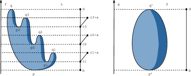
Let $f(q_{i})-f(p_{i})=a$ , $i=1,2,3$ . Up to re-parameterization of ${\mathcal{M}}$ , we have ${\|f-g\|}_{C^{0}}=\frac{a}{2}$ . The deformation $T$ that deletes the three edges $e(p_{i},q_{i})\in E(\Gamma_{f})$ has cost $c(T)=3\cdot\frac{a}{2}$ , implying $d_{E}((\Gamma_{f},\ell_{f}),(\Gamma_{g},\ell_{g}))\leq 3\cdot{\|f-g\|}_{C^{0}}$ . On the other hand, applying Proposition 3.4 we see that actually $d_{E}((\Gamma_{f},\ell_{f}),(\Gamma_{g},\ell_{g}))\leq{\|f-g\|}_{C^{0}}$ . Indeed, for every $0<\epsilon<\frac{a}{2}$ , we can apply to $(\Gamma_{f},\ell_{f})$ a deformation of type (R), that relabels the vertices $p_{i},q_{i}$ , $i=1,2,3$ , in such a way that $\ell_{f}(p_{i})$ is increased by $\frac{a}{2}-\epsilon$ , and $\ell_{f}(q_{i})$ is decreased by $\frac{a}{2}-\epsilon$ , composed with three deformations of type (D) that delete $p_{i}$ , $q_{i}$ and the edge $e(p_{i},q_{i})$ , for $i=1,2,3$ respectively.

In order to prove Theorem 4.1, we consider the set $\mathcal{F}({\mathcal{M}})$ of smooth real-valued functions on ${\mathcal{M}}$ endowed with the $C^{2}$ topology, which may be defined as follows. Let $\{U_{\alpha}\}$ be a coordinate covering of ${\mathcal{M}}$ with coordinate maps $\varphi_{\alpha}:U_{\alpha}\to\mathbb{R}^{2}$ , and let $\{C_{\alpha}\}$ be a compact refinement of $\{U_{\alpha}\}$ . For every positive constant $\delta>0$ and every $f\in\mathcal{F}({\mathcal{M}})$ , define $N(f,\delta)$ as the subset of $\mathcal{F}({\mathcal{M}})$ consisting of all maps $g$ such that, denoting $f_{\alpha}=f\circ\varphi_{\alpha}^{-1}$ and $g_{\alpha}=g\circ\varphi_{\alpha}^{-1}$ , it holds that $\underset{i+j\leq 2}{\max}\left|\frac{\partial^{i+j}}{\partial x^{i}\partial y^{j}}(f_{\alpha}-g_{\alpha})\right|<\delta$ at all points of $\varphi_{\alpha}(C_{\alpha})$ . The $C^{2}$ topology is the topology obtained by taking the sets $N(f,\delta)$ as a base of neighborhoods.

Next we consider the strata $\mathcal{F}^{0}({\mathcal{M}})$ and $\mathcal{F}^{1}({\mathcal{M}})$ of the natural stratification of $\mathcal{F}({\mathcal{M}})$ , as presented by Cerf in [4].

•

The stratum $\mathcal{F}^{0}({\mathcal{M}})$ is the set of simple Morse functions.
•
The stratum $\mathcal{F}^{1}({\mathcal{M}})$ is the disjoint union of two sets $\mathcal{F}^{1}_{\alpha}({\mathcal{M}})$ and $\mathcal{F}^{1}_{\beta}({\mathcal{M}})$ , where
- –
  
  $\mathcal{F}^{1}_{\alpha}({\mathcal{M}})$ is the set of functions whose critical levels contain exactly one critical point, and the critical points are all non-degenerate, except exactly one.
- –
  
  $\mathcal{F}^{1}_{\beta}({\mathcal{M}})$ is the set of Morse functions whose critical levels contain at most one critical point, except for one level containing exactly two critical points.

$\mathcal{F}^{1}({\mathcal{M}})$ is a sub-manifold of co-dimension 1 of $\mathcal{F}^{0}({\mathcal{M}})\cup\mathcal{F}^{1}({\mathcal{M}})$ , and the complement of $\mathcal{F}^{0}({\mathcal{M}})\cup\mathcal{F}^{1}({\mathcal{M}})$ in $\mathcal{F}({\mathcal{M}})$ is of co-dimension greater than 1. Hence, given two functions $f,g\in\mathcal{F}^{0}({\mathcal{M}})$ , we can always find $\widehat{f},\widehat{g}\in\mathcal{F}^{0}({\mathcal{M}})$ arbitrarily near to $f,g$ , respectively, for which

•

$\widehat{f}$ , $\widehat{g}$ are RL-equivalent to $f$ , $g$ , respectively,

and the path $h(\lambda)=(1-\lambda)\widehat{f}+\lambda\widehat{g}$ , with $\lambda\in[0,1]$ , is such that

•

$h(\lambda)$ belongs to $\mathcal{F}^{0}({\mathcal{M}})\cup\mathcal{F}^{1}({\mathcal{M}})$ for every $\lambda\in[0,1]$ ;
•

$h(\lambda)$ is transversal to $\mathcal{F}^{1}({\mathcal{M}})$ .

As a consequence, $h(\lambda)$ belongs to $\mathcal{F}^{1}({\mathcal{M}})$ for at most a finite collection of values $\lambda$ , and does not traverse strata of co-dimension greater than 1 (see, e.g., [9]).

With these preliminaries set, the stability theorem will be proven by considering a path that connects $f$ to $g$ via $\widehat{f}$ , $h(\lambda)$ , and $\widehat{g}$ as aforementioned. This path can be split into a finite number of linear sub-paths whose endpoints are such that the stability theorem holds on them, as will be shown in some preliminary lemmas. In conclusion, Theorem 4.1 will be proven by applying the triangle inequality of the edit distance.

In the following preliminary lemmas, $f$ and $g$ belong to $\mathcal{F}^{0}({\mathcal{M}})$ and $h:[0,1]\to\mathcal{F}({\mathcal{M}})$ denotes their convex linear combination: $h(\lambda)=(1-\lambda)f+\lambda g$ .

Lemma 4.2.

${\|h(\lambda^{\prime})-h(\lambda^{\prime\prime})\|}_{C^{0}}=|\lambda^{\prime}-\lambda^{\prime\prime}|\cdot{\|f-g\|}_{C^{0}}$ for every $\lambda^{\prime},\lambda^{\prime\prime}\in[0,1]$ .

Proof.

	$\displaystyle{\\|h(\lambda^{\prime})-h(\lambda^{\prime\prime})\\|}_{C^{0}}$	$\displaystyle=$	$\displaystyle{\\|(1-\lambda^{\prime})f+\lambda^{\prime}g-(1-\lambda^{\prime\prime})f-\lambda^{\prime\prime}g\\|}_{C^{0}}$
		$\displaystyle=$	$\displaystyle{\\|(\lambda^{\prime\prime}-\lambda^{\prime})f-(\lambda^{\prime\prime}-\lambda^{\prime})g\\|}_{C^{0}}=\|\lambda^{\prime}-\lambda^{\prime\prime}\|\cdot{\\|f-g\\|}_{C^{0}}.$

∎

Lemma 4.3.

If $h(\lambda)\in\mathcal{F}^{0}({\mathcal{M}})$ for every $\lambda\in[0,1]$ , then $d_{E}((\Gamma_{f},\ell_{f}),(\Gamma_{g},\ell_{g}))\leq{\|f-g\|}_{C^{0}}.$

Proof.

The statement can be proved in the same way as [7, Prop. 5.4]. ∎

Lemma 4.4.

Let $h(\lambda)$ intersect $\mathcal{F}^{1}({\mathcal{M}})$ transversely at $h(\overline{\lambda})$ , $0<\overline{\lambda}<1$ , and nowhere else. Then, for every constant value $\delta>0$ , there exist two real numbers $\lambda^{\prime},\lambda^{\prime\prime}$ with $0<\lambda^{\prime}<\overline{\lambda}<\lambda^{\prime\prime}<1$ , such that

d_{E}((\Gamma_{h(\lambda^{\prime})},\ell_{h(\lambda^{\prime})}),(\Gamma_{h(\lambda^{\prime\prime})},\ell_{h(\lambda^{\prime\prime})}))\leq\delta.

Proof.

In this proof we use the notion of universal deformation of a function. More details on universal deformations may be found in [16, 21]. In particular, we will consider two different universal deformations $F$ and $G$ of $\overline{h}=h(\overline{\lambda})$ . Firstly we show how $F$ and $G$ yield the claim, and then construct them.

We use the fact that, being two universal deformations of $\overline{h}\in\mathcal{F}^{1}({\mathcal{M}})$ , $F$ and $G$ are equivalent. This means that there exist a diffeomorphism $\eta(s)$ of $\mathbb{R}$ with $\eta(0)=0$ , and a local diffeomorphism $\phi(s,(x,y))$ , with $\phi(s,(x,y))=(\eta(s),\psi(\eta(s),(x,y)))$ and $\phi(0,(x,y))=(0,(x,y))$ , such that $F=(\eta^{*}G)\circ\phi$ . Hence, apart from the labels, the Reeb graphs of $F(s,\cdot)$ and $G(\eta(s),\cdot)$ are isomorphic. Moreover, the difference the labels at corresponding vertices in the Reeb graphs of $F(s,\cdot)$ and $G(\eta(s),\cdot)$ continuously depends on $s$ , and is $0$ for $s=0$ . Therefore, for every $\delta>0$ , taking $|s|$ sufficiently small, it is possible to transform the labeled Reeb graph of $F(s,\cdot)$ into that of $G(\eta(s),\cdot)$ , or viceversa, by a deformation of type (R) whose cost is not greater than $\delta/3$ . Moreover, as equality (4.3) will show, for every $\delta>0$ , $|s|$ can be taken sufficiently small that the distance between the labeled Reeb graphs of $G(\eta(s),\cdot)$ and $G(\eta(-s),\cdot)$ is not greater that $\delta/3$ . Thus, applying the triangle inequality, we deduce that, for every $\delta>0$ , there exists a sufficiently small $s>0$ such that the distance between the labeled Reeb graphs of $F(s,\cdot)$ and $F(-s,\cdot)$ is not greater than $\delta$ . The claim follows taking $\lambda^{\prime}=\overline{\lambda}-s$ and $\lambda^{\prime\prime}=\overline{\lambda}+s$ .

We now construct the universal deformations $F(s,p)$ and $G(s,p)$ , with $s\in\mathbb{R}$ and $p\in{\mathcal{M}}$ . We define $F$ by setting $F(s,p)=\overline{h}(p)+s\cdot(g-f)(p)$ . This deformation is universal because $h(\lambda)$ intersects $\mathcal{F}^{1}({\mathcal{M}})$ transversely at $h(\overline{\lambda})$ . In order to construct $G$ , let us consider separately the two cases $\mathcal{F}^{1}_{\alpha}({\mathcal{M}})$ and $\mathcal{F}^{1}_{\beta}({\mathcal{M}})$ .

Case $\overline{h}\in\mathcal{F}^{1}_{\alpha}({\mathcal{M}})$ : Let $\overline{p}$ be the sole degenerate critical point of $\overline{h}$ . Let $(x,y)$ be a suitable local coordinate system around $\overline{p}$ in which the canonical expression of $\overline{h}$ is $\overline{h}(x,y)=\overline{h}(\overline{p})\pm x^{2}+y^{3}$ .

Let $\omega:{\mathcal{M}}\to\mathbb{R}$ be a smooth function equal to $1$ in a neighborhood of $\overline{p}$ , which decreases moving from $\overline{p}$ , and whose support is contained in the chosen coordinate chart around $\overline{p}$ . Finally, let $G(\eta,(x,y))=\overline{h}(x,y)-\eta\cdot\omega(x,y)\cdot y$ , where $\eta\in\mathbb{R}$ . For $\eta<0$ , $G(\eta,\cdot)$ has no critical points in the support of $\omega$ and is equal to $\overline{h}$ everywhere else, while, for $\eta>0$ , $G(\eta,\cdot)$ has exactly two critical points in the support of $\omega$ , precisely $p_{1}=\left(0,-\sqrt{\frac{\eta}{3}}\right)$ and $p_{2}=\left(0,\sqrt{\frac{\eta}{3}}\right)$ , and is equal to $\overline{h}$ everywhere else (see Figure 6). Therefore, for every $\eta>0$ sufficiently small, the labeled Reeb graph of $G(-\eta,\cdot)$ can be transformed into that of $G(\eta,\cdot)$ by an elementary deformation $T$ of type (B). Obviously, in the case $\eta<0$ , the deformation we consider is of type (D).

By Definition 3.1 and Proposition 3.2, a direct computation shows that the cost of $T$ is

(4.1)

\displaystyle c(T)

\displaystyle=

\displaystyle 2\cdot\left(\frac{|\eta|}{3}\right)^{3/2}.

Case $\overline{h}\in\mathcal{F}^{1}_{\beta}({\mathcal{M}})$ : Let $\overline{p}$ and $\overline{q}$ be the critical points of $\overline{h}$ such that $\overline{h}(\overline{p})=\overline{h}(\overline{q})$ . Since $\overline{p}$ is non-degenerate, there exists a suitable local coordinate system $(x,y)$ around $\overline{p}$ in which the canonical expression of $\overline{h}$ is $\overline{h}(x,y)=\overline{h}(\overline{p})+x^{2}+y^{2}$ if $\overline{p}$ is a minimum, or $\overline{h}(x,y)=\overline{h}(\overline{p})-x^{2}-y^{2}$ if $\overline{p}$ is a maximum, or $\overline{h}(x,y)=\overline{h}(\overline{p})\pm x^{2}\mp y^{2}$ if $\overline{p}$ is a saddle point. Let $\omega:{\mathcal{M}}\to\mathbb{R}$ be a smooth function equal to $1$ in a neighborhood of $\overline{p}$ , which decreases moving from $\overline{p}$ , and whose support is contained in the coordinate chart around $\overline{p}$ in which $\overline{h}$ has one of the above expressions. Finally, let $G(\eta,(x,y))=\overline{h}(x,y)+\eta\cdot\omega(x,y)$ , where $\eta=\eta(s)$ , $s\in\mathbb{R}$ . For every $\eta\in\mathbb{R}$ , with $|\eta|$ sufficiently small, $G(\eta,\cdot)$ has the same critical points, with the same indices, as $\overline{h}$ . As for critical values, they are the same as well, apart from the value taken at $\overline{p}$ : $G(\eta,\overline{p})=\overline{h}(\overline{p})+\eta$ .

We distinguish the following two situations illustrated in Figures 7 and 8:

(1)

the points $\overline{p}$ and $\overline{q}$ belong to two different connected components of $\overline{h}^{-1}(\overline{h}(\overline{p}))$ ;

Figure 7. Two critical points in different connected components of the same critical level. The dark (resp. light) regions correspond to points below (resp. above) this critical level. Possibly inverting the colors of one or both the components, we have all the possible cases.
(2)

the points $\overline{p}$ and $\overline{q}$ belong to the same connected component of $\overline{h}^{-1}(\overline{h}(\overline{p}))$ .

Figure 8. Two critical points in the same connected component of the same critical level. The dark (resp. light) regions correspond to points below (resp. above) this critical level. Possibly inverting the colors of this component, we have all the possible cases.

In the situation (1), for every $\eta>0$ sufficiently small, the labeled Reeb graphs of $G(-\eta,\cdot)$ and $G(\eta,\cdot)$ can be obtained one from the other through an elementary deformation $T$ of type (R) (see, e.g., Figure 9).

In the situation (2), the following elementary deformations need to be considered:

•

If $\overline{p}$ and $\overline{q}$ are as in Figure 8 $(a)$ , then, for every $\eta>0$ sufficiently small, the labeled Reeb graphs of $G(-\eta,\cdot)$ and $G(\eta,\cdot)$ can be obtained one from the other through an elementary deformation $T$ of type (K₁) (see, e.g., Figure 11).
•

If $\overline{p}$ and $\overline{q}$ are as in Figure 8 $(b)$ , then, for every $\eta>0$ sufficiently small, the labeled Reeb graphs of $G(-\eta,\cdot)$ and $G(\eta,\cdot)$ can be obtained one from the other through an elementary deformation $T$ of type (K₃) or (K₂) (see, e.g., Figure 11).
•

If $\overline{p}$ and $\overline{q}$ are as in Figure 8 $(c)$ or $(d)$ , then, for every $\eta>0$ sufficiently small, the labeled Reeb graphs of $G(-\eta,\cdot)$ and $G(\eta,\cdot)$ can be obtained one from the other through an elementary deformation $T$ of type (R) (see, e.g., Figures 13-13).

In all the cases, for every $\eta>0$ sufficiently small, the cost of the considered deformation $T$ is:

(4.2)

\displaystyle c(T)

\displaystyle=

\displaystyle|\overline{h}(\overline{p})-\eta-(\overline{h}(\overline{p})+\eta)|=2\eta.

In conclusion, from equalities (4.1) and (4.2), for every $\eta>0$ sufficiently small, we get

d_{E}((\Gamma_{G(-\eta,\cdot)},\ell_{G(-\eta,\cdot)}),(\Gamma_{G(\eta,\cdot)},\ell_{G(\eta,\cdot)}))\leq\max\left\{2\cdot\left(\frac{\eta}{3}\right)^{3/2},2\eta\right\}.

Thus, for every $\delta>0$ , we can always take a value $|s|$ sufficiently small that $|\eta(s)|$ results small enough to imply the following inequality:

(4.3)

\displaystyle d_{E}((\Gamma_{G(-\eta(s),\cdot)},\ell_{G(-\eta(s),\cdot)}),(\Gamma_{G(\eta(s),\cdot)},\ell_{G(\eta(s),\cdot)}))\leq\delta/3.

∎

Lemma 4.5.

If $h(\lambda)$ belongs to $\mathcal{F}^{0}({\mathcal{M}})$ for every $\lambda\in[0,1]$ apart from one value $0<\overline{\lambda}<1$ at which $h$ transversely intersects $\mathcal{F}^{1}({\mathcal{M}})$ , then $d_{E}((\Gamma_{f},\ell_{f}),(\Gamma_{g},\ell_{g}))\leq{\|f-g\|}_{C^{0}}.$

Proof.

Let $\overline{h}=h(\overline{\lambda})$ . By Lemma 4.4, for every real number $\delta>0$ ,we can find two values $0<\lambda^{\prime}<\overline{\lambda}<\lambda^{\prime\prime}<1$ such that $d_{E}((\Gamma_{h(\lambda^{\prime})},\ell_{h(\lambda^{\prime})}),(\Gamma_{h(\lambda^{\prime\prime})},\ell_{h(\lambda^{\prime\prime})}))\leq\delta.$

Applying the triangle inequality, we have:

	$\displaystyle d_{E}((\Gamma_{f},\ell_{f}),(\Gamma_{g},\ell_{g}))$	$\displaystyle\leq$	$\displaystyle d_{E}((\Gamma_{f},\ell_{f}),(\Gamma_{h(\lambda^{\prime})},\ell_{h(\lambda^{\prime})}))+d_{E}((\Gamma_{h(\lambda^{\prime})},\ell_{h(\lambda^{\prime})}),(\Gamma_{h(\lambda^{\prime\prime})},\ell_{h(\lambda^{\prime\prime})}))$
			$\displaystyle+d_{E}((\Gamma_{h(\lambda^{\prime\prime})},\ell_{h(\lambda^{\prime\prime})}),(\Gamma_{g},\ell_{g})).$

Moreover, we get

d_{E}((\Gamma_{f},\ell_{f}),(\Gamma_{h(\lambda^{\prime})},\ell_{h(\lambda^{\prime})}))\leq\|f-h(\lambda^{\prime})\|_{C^{0}}=\lambda^{\prime}\cdot\|f-g\|_{C^{0}},

and

d_{E}((\Gamma_{h(\lambda^{\prime\prime})},\ell_{h(\lambda^{\prime\prime})}),(\Gamma_{g},\ell_{g}))\leq\|h(\lambda^{\prime\prime})-g\|_{C^{0}}=(1-\lambda^{\prime\prime})\cdot\|f-g\|_{C^{0}},

where the inequalities follow from Lemma 4.3, and equalities from Lemma 4.2 with $f=h(0),g=h(1)$ . Hence,

d_{E}((\Gamma_{f},\ell_{f}),(\Gamma_{g},\ell_{g}))\leq(1+\lambda^{\prime}-\lambda^{\prime\prime})\cdot\|f-g\|_{C^{0}}+\delta.

In conclusion, given that $0<\lambda^{\prime}<\lambda^{\prime\prime}$ , the inequality $d_{E}((\Gamma_{f},\ell_{f}),(\Gamma_{g},\ell_{g}))\leq\|f-g\|_{C^{0}}+\delta$ holds. This yields the claim by the arbitrariness of $\delta$ . ∎

We are now ready to prove the stability Theorem 4.1.

Proof of Theorem 4.1.

Recall from [12] that $\mathcal{F}^{0}({\mathcal{M}})$ is open in $\mathcal{F}({\mathcal{M}})$ endowed with the $C^{2}$ topology. Thus, for every sufficiently small real number $\delta>0$ , the neighborhoods $N(f,\delta)$ and $N(g,\delta)$ are contained in $\mathcal{F}^{0}({\mathcal{M}})$ . Take $\widehat{f}\in N(f,\delta)$ and $\widehat{g}\in N(g,\delta)$ such that the path $h:[0,1]\to\mathcal{F}({\mathcal{M}})$ , with $h(\lambda)=(1-\lambda)\widehat{f}+\lambda\widehat{g}$ , belongs to $\mathcal{F}^{0}({\mathcal{M}})$ for every $\lambda\in[0,1]$ , except for at most a finite number $n$ of values, $\mu_{1},\mu_{2},\dots,\mu_{n}$ , at which $h$ transversely intersects $\mathcal{F}^{1}({\mathcal{M}})$ . We begin by proving our statement for $\widehat{f}$ and $\widehat{g}$ , and then show its validity for $f$ and $g$ . We proceed by induction on $n$ . If $n=0$ or $n=1$ , the inequality $d_{E}((\Gamma_{\widehat{f}},\ell_{\widehat{f}}),(\Gamma_{\widehat{g}},\ell_{\widehat{g}}))\leq{\|\widehat{f}-\widehat{g}\|}_{C^{0}}$ holds because of Lemma 4.3 or 4.5, respectively. Let us assume the claim is true for $n\geq 1$ , and prove it for $n+1$ . Let $0<\mu_{1}<\lambda_{1}<\mu_{2}<\lambda_{2}<\ldots<\mu_{n}<\lambda_{n}<\mu_{n+1}<1$ , with $h(0)=\widehat{f}$ , $h(1)=\widehat{g}$ , $h(\mu_{i})\in\mathcal{F}^{1}({\mathcal{M}})$ , for every $i=1,\ldots,n+1$ , and $h(\lambda_{j})\in\mathcal{F}^{0}({\mathcal{M}})$ , for every $j=1,\ldots,n$ . We consider $h$ as the concatenation of the paths $h^{1},h^{2}:[0,1]\to\mathcal{F}({\mathcal{M}})$ , defined, respectively, as $h^{1}(\lambda)=(1-\lambda)\widehat{f}+\lambda h(\lambda_{n})$ , and $h^{2}(\lambda)=(1-\lambda)h(\lambda_{n})+\lambda\widehat{g}$ . The path $h^{1}$ transversally intersect $\mathcal{F}^{1}({\mathcal{M}})$ at $n$ values $\mu_{1},\ldots,\mu_{n}$ . Hence, by the inductive hypothesis, we have $d_{E}((\Gamma_{\widehat{f}},\ell_{\widehat{f}}),(\Gamma_{h(\lambda_{n})},\ell_{h(\lambda_{n})}))\leq{\|\widehat{f}-h(\lambda_{n})\|}_{C^{0}}$ . Moreover, the path $h^{2}$ transversally intersect $\mathcal{F}^{1}({\mathcal{M}})$ only at the value $\mu_{n+1}$ . Consequently, by Lemma 4.5, we have $d_{E}((\Gamma_{h(\lambda_{n})},\ell_{h(\lambda_{n})}),(\Gamma_{\widehat{g}},\ell_{\widehat{g}}))\leq{\|h(\lambda_{n})-\widehat{g}\|}_{C^{0}}$ . Using the triangle inequality and Lemma 4.2, we can conclude that:

(4.4)		$\displaystyle d_{E}((\Gamma_{\widehat{f}},\ell_{\widehat{f}}),(\Gamma_{\widehat{g}},\ell_{\widehat{g}}))$	$\displaystyle\leq$	$\displaystyle d_{E}((\Gamma_{\widehat{f}},\ell_{\widehat{f}}),(\Gamma_{h(\lambda_{n})},\ell_{h(\lambda_{n})}))+d_{E}((\Gamma_{h(\lambda_{n})},\ell_{h(\lambda_{n})}),(\Gamma_{\widehat{g}},\ell_{\widehat{g}}))$
(4.4)			$\displaystyle\leq$	$\displaystyle\lambda_{n}{\\|\widehat{f}-\widehat{g}\\|}_{C^{0}}+(1-\lambda_{n}){\\|\widehat{f}-\widehat{g}\\|}_{C^{0}}={\\|\widehat{f}-\widehat{g}\\|}_{C^{0}}.$

Let us now estimate $d_{E}((\Gamma_{f},\ell_{f}),(\Gamma_{g},\ell_{g}))$ . By the triangle inequality, we have:

d_{E}((\Gamma_{f},\ell_{f}),(\Gamma_{g},\ell_{g}))\leq d_{E}((\Gamma_{f},\ell_{f}),(\Gamma_{\widehat{f}},\ell_{\widehat{f}}))+d_{E}((\Gamma_{\widehat{f}},\ell_{\widehat{f}}),(\Gamma_{\widehat{g}},\ell_{\widehat{g}}))+d_{E}((\Gamma_{\widehat{g}},\ell_{\widehat{g}}),(\Gamma_{g},\ell_{g})).

Since $\widehat{f}\in N(f,\delta)\subset\mathcal{F}^{0}({\mathcal{M}})$ and $\widehat{g}\in N(g,\delta)\subset\mathcal{F}^{0}({\mathcal{M}})$ , the following facts hold: $(a)$ for every $\lambda\in[0,1]$ , $(1-\lambda)f+\lambda\widehat{f},(1-\lambda)g+\lambda\widehat{g}\in\mathcal{F}^{0}({\mathcal{M}})$ ; $(b)$ ${\|f-\widehat{f}\|}_{C^{0}}\leq\delta$ and ${\|\widehat{g}-g\|}_{C^{0}}\leq\delta$ . Hence, from $(a)$ and Lemma 4.3, we get $d_{E}((\Gamma_{f},\ell_{f}),(\Gamma_{\widehat{f}},\ell_{\widehat{f}}))\leq{\|f-\widehat{f}\|}_{C^{0}}$ , and $d_{E}((\Gamma_{g},\ell_{g}),(\Gamma_{\widehat{g}},\ell_{\widehat{g}}))\leq{\|\widehat{g}-g\|}_{C^{0}}$ . Using inequality (4.4) and the triangle inequality of $\|\cdot\|_{C^{0}}$ , we deduce that

	$\displaystyle d_{E}((\Gamma_{f},\ell_{f}),(\Gamma_{g},\ell_{g}))$	$\displaystyle\leq$	$\displaystyle{\\|f-\widehat{f}\\|}_{C^{0}}+\\|\widehat{f}-\widehat{g}\\|_{C^{0}}+{\\|\widehat{g}-g\\|}_{C^{0}}$
		$\displaystyle\leq$	$\displaystyle\\|f-g\\|_{C^{0}}+2({\\|f-\widehat{f}\\|}_{C^{0}}+{\\|\widehat{g}-g\\|}_{C^{0}}).$

Hence, from $(b)$ , we have $d_{E}((\Gamma_{f},\ell_{f}),(\Gamma_{g},\ell_{g}))\leq\|f-g\|_{C^{0}}+4\delta$ . This yields the conclusion by the arbitrariness of $\delta$ . ∎

5. Relationships with other stable metrics

In this section, we consider relationships between the edit distance and other metrics for shape comparison: the natural pseudo-distance between functions [8], the functional distortion distance between Reeb graphs [1], and the bottleneck distance between persistence diagrams [6]. More precisely, the main result we are going to show states that the natural pseudo-distance between two simple Morse functions $f$ and $g$ and the edit distance between the corresponding Reeb graphs actually coincide (Theorem 5.6). As a consequence, we deduce that the edit distance is a metric (Corollary 5.7), and that it is more discriminative than the bottleneck distance between persistence diagrams (Corollary 5.8) and the functional distortion distance between Reeb graphs (Corollary 5.9).

The natural pseudo-distance is a dissimilarity measure between any two functions defined on the same compact manifold obtained by minimizing the difference in the functions via a re-parameterization of the manifold [8]. In general, the natural pseudo-distance is only a pseudo-metric. However it turns out to be a metric in some particular cases such as the case of simple Morse functions on a smooth closed connected surface, considered up to $R$ -equivalence, as proved in [3]. We give the definition in this context.

Definition 5.1.

The natural pseudo-distance between $R$ -equivalence classes of simple Morse functions $f,g$ on the same surface ${\mathcal{M}}$ is defined as

d_{N}([f],[g])=\underset{\xi\in{\mathcal{D}}({\mathcal{M}})}{\inf}\|f-g\circ\xi\|_{C^{0}},

where ${\mathcal{D}}({\mathcal{M}})$ is the set of self-diffeomorphisms on ${\mathcal{M}}$ .

In order to study $d_{N}$ , it is often useful to consider the following fact.

Proposition 5.2.

Letting ${\mathcal{H}}({\mathcal{M}})$ be the set of self-homeomorphisms on ${\mathcal{M}}$ , it holds that $d_{N}([f],[g])=\underset{\xi\in{\mathcal{H}}({\mathcal{M}})}{\inf}\|f-g\circ\xi\|_{C^{0}}$ .

Proof.

Let $d=d_{N}([f],[g])$ . Clearly $\underset{\xi\in{\mathcal{H}}({\mathcal{M}})}{\inf}\|f-g\circ\xi\|_{C^{0}}\leq d$ . By contradiction, assuming that $\underset{\xi\in{\mathcal{H}}({\mathcal{M}})}{\inf}\|f-g\circ\xi\|_{C^{0}}<d$ , there exists a homeomorphism $\overline{\xi}$ such that $\|f-g\circ\overline{\xi}\|_{C^{0}}<d$ . On the other hand, by [25, Cor. 1.18], for every metric $\delta$ on ${\mathcal{M}}$ and for every $n\in\mathbb{N}$ , there exists a diffeomorphism $\xi_{n}:{\mathcal{M}}\to{\mathcal{M}}$ such that $\delta(\xi_{n}(p),\overline{\xi}(p))<1/n$ , for every $p\in{\mathcal{M}}$ . Hence, by the continuity of $g$ , and applying the reverse triangle inequality, we deduce that

\lim_{n\to\infty}\left|\|f-g\circ\overline{\xi}\|_{C^{0}}-\|f-g\circ\xi_{n}\|_{C^{0}}\right|\leq\lim_{n\to\infty}\|g\circ\xi_{n}-g\circ\overline{\xi}\|_{C^{0}}=0.

Therefore, for $n$ sufficiently large, there exists a diffeomorphism $\xi_{n}$ such that $\|f-g\circ\xi_{n}\|_{C^{0}}<d$ , yielding a contradiction. ∎

The following Lemmas 5.3-5.5 state that the cost of each elementary deformation upper-bounds the natural pseudo-distance. Their proofs deploy the concepts of elementary cobordism and rearrangement, whose detailed treatment can be found in [18].

Lemma 5.3.

For every elementary deformation $T\in{\mathcal{T}}((\Gamma_{f},\ell_{f}),(\Gamma_{g},\ell_{g}))$ of type (R), $c(T)\geq d_{N}([f],[g])$ .

Proof.

Since $T$ is of type (R), there exists an edge preserving bijection $\Phi:V(\Gamma_{f})\to V(\Gamma_{g})$ . Hence, $f$ and $g$ have the same number of critical points of the same type: $K_{f}=\{p_{1},\ldots,p_{n}\}$ , $K_{g}=\{p^{\prime}_{1},\ldots,p^{\prime}_{n}\}$ , with $\Phi(p_{i})=p^{\prime}_{i}$ , and $p_{i},p^{\prime}_{i}$ both being of index 0,1, or 2.

Let $c_{i}=f(p_{i})$ and $c^{\prime}_{i}=g(p_{i}^{\prime})$ for $i=1,\ldots,n$ . We shall construct a homeomorphism $\xi:{\mathcal{M}}\to{\mathcal{M}}$ such that $\xi_{|K_{f}}=\Phi$ and ${\|f-g\circ\xi\|}_{C^{0}}=\underset{i=1,\ldots,n}{\max}|c_{i}-c_{i}^{\prime}|=c(T)$ . By Proposition 5.2, this will yield the claim.

Let us endow ${\mathcal{M}}$ with a Riemannian metric, and consider the smooth vector field $X=-\frac{\nabla f}{\|\nabla f\|^{2}}$ on ${\mathcal{M}}\setminus K_{f}$ , and the smooth vector field $Y=\frac{\nabla g}{\|\nabla g\|^{2}}$ on ${\mathcal{M}}\setminus K_{g}$ . Let us denote by $\varphi_{t}(p)$ and $\psi_{t}(p)$ the flow lines defined by $X$ and $Y$ , on ${\mathcal{M}}\setminus K_{f}$ and ${\mathcal{M}}\setminus K_{g}$ , respectively. We observe that $f$ strictly decreases along $X$ -trajectories, while $g$ strictly increases along $Y$ -trajectories. Moreover, no two $X$ -trajectories (resp. $Y$ -trajectories) pass through the same $p$ . Hence, $\varphi_{t}(p)$ and $\psi_{t}(p)$ are injective functions of $t$ and $p$ , separately. By [19, Prop. 1.3], $\varphi$ and $\psi$ are continuous in $t$ and $p$ when restricted to compact submanifolds of ${\mathcal{M}}\setminus K_{f}$ and ${\mathcal{M}}\setminus K_{g}$ , respectively.

Let us fix a real number $\varepsilon>0$ sufficiently small so that, for $i=1,\ldots,n$ , $f^{-1}([c_{i}-\varepsilon,c_{i}+\varepsilon])\cap K_{f}=\{p_{i}\}$ and $g^{-1}([c^{\prime}_{i}-\varepsilon,c^{\prime}_{i}+\varepsilon])\cap K_{g}=\{p^{\prime}_{i}\}$ .

In order to construct the desired homeomorphism $\xi$ on ${\mathcal{M}}$ , the main idea is to cut ${\mathcal{M}}$ into cobordisms and define suitable homeomorphisms on each of these cobordisms that can be glued together to obtain $\xi$ . The fact that $\xi$ is not required to be differentiable but only continuous facilitates the gluing process.

Let us consider the cobordisms obtained cutting ${\mathcal{M}}$ along the level curves $f^{-1}(c_{i}\pm\varepsilon)$ and $g^{-1}(c^{\prime}_{i}\pm\varepsilon)$ for $i=1,\ldots,n$ . According to whether these cobordisms contain points of maximum, minimum, saddle points, or no critical points at all, we treat the cases differently.

Case 1: Let $p_{i},p_{i}^{\prime}$ be points of maximum or minimum of $f$ and $g$ , respectively. Let $D=D_{i}$ (resp. $D^{\prime}=D_{i}^{\prime}$ , ) be the connected component of $f^{-1}([c_{i}-\varepsilon,c_{i}+\varepsilon])$ (resp. $g^{-1}([c^{\prime}_{i}-\varepsilon,c^{\prime}_{i}+\varepsilon])$ ) that contains $p_{i}$ (resp. $p^{\prime}_{i}$ ). $D$ and $D^{\prime}$ are topolological disks. Let $\sigma^{D}:\partial D\to\partial D^{\prime}$ be a given homeomorphism between the boundaries of $D$ and $D^{\prime}$ .

Claim 1. There exists a homeomorphism $\xi^{D}:D\to D^{\prime}$ such that:

$(a_{1})$

$\xi^{D}|_{\partial D}=\sigma^{D}$ ;
$(b_{1})$

$\underset{p\in D}{\max}|f(p)-g\circ\xi^{D}(p)|=|c_{i}-c^{\prime}_{i}|.$

Proof of Claim 1. We first prove Claim 1 for maxima. We set $\xi^{D}(p_{i})=p^{\prime}_{i}$ , and, for every $p\in D\setminus\{p_{i}\}$ , $\xi^{D}(p)=p^{\prime}$ , where $p^{\prime}=\psi_{f(p)-c_{i}+\varepsilon}\circ\sigma^{D}\circ\varphi_{f(p)-c_{i}+\varepsilon}(p)$ . In plain words, for each $p\in D$ we follow the $X$ -flow downwards until the intersection with $f^{-1}(c_{i}-\varepsilon)$ ; then we apply the homeomorphism $\sigma^{D}$ to go from $f^{-1}(c_{i}-\varepsilon)$ to $g^{-1}(c_{i}^{\prime}-\varepsilon)$ ; finally, we follow the $Y$ -flow upwards.

The function $\xi^{D}$ is injective as can be seen using the aforementioned injectivity property of $\varphi$ and $\psi$ . Moreover, $\xi^{D}$ is surjective because, for every $p\in D\setminus\{p_{i}\}$ , there exists a flow line passing for $p$ . Furthermore, $\xi^{D}$ is continuous on $D\setminus\{p_{i}\}$ because composition of continuous functions. The continuity can be extended to the whole $D$ as can be seen taking a sequence $(q_{j})$ in $D\setminus\{p_{i}\}$ converging to $p_{i}$ . Since $\lim_{j}f(q_{j})=c_{i}$ , by construction of $\xi^{D}$ it holds that $\lim_{j}g(\xi^{D}(q_{j}))=c_{i}^{\prime}$ . We see that $\lim_{j}\xi^{D}(q_{j})=p_{i}^{\prime}$ because $p_{i}^{\prime}$ is the only point of $D^{\prime}$ where $g$ takes value equal to $c_{i}^{\prime}$ ,. Therefore $\xi^{D}$ is continuous on $D$ . Moreover, since $\xi^{D}$ is a continuous bijection from a compact space to a Hausdorff space, it is a homeomorphism. Finally, property $(a_{1})$ holds by construction and property $(b_{1})$ holds because, for every $p\in D$ , $g(\xi^{D}(p))=f(p)+c_{i}^{\prime}-c_{i}$ .

To prove Claim 1 when $p_{i},p^{\prime}_{i}$ are minimum points of $f$ and $g$ , it is sufficient to replace $\varphi_{f(p)-c_{i}+\varepsilon}(p)$ and $\psi_{f(p)-c_{i}+\varepsilon}(p)$ by $\varphi_{f(p)-c_{i}-\varepsilon}(p)$ and $\psi_{f(p)-c_{i}-\varepsilon}(p)$ , respectively.

Case 2: Let $p_{i},p^{\prime}_{i}$ be two splitting saddle points or two joining saddle points of $f$ and $g$ , respectively, and let $P$ and $P^{\prime}$ be the connected component of $f^{-1}([c_{i}-\varepsilon,c_{i}+\varepsilon])$ and $g^{-1}([c^{\prime}_{i}-\varepsilon,c^{\prime}_{i}+\varepsilon])$ , respectively, that contain $p_{i}$ and $p^{\prime}_{i}$ . Let $\sigma^{P}:\partial^{-}P\to\partial^{-}P^{\prime}$ be a given homeomorphism between the lower boundaries of $P$ and $P^{\prime}$ .

Claim 2. There exists a homeomorphism $\xi^{P}:P\to P^{\prime}$ such that:

$(a_{2})$

$\xi^{P}|_{\partial^{-}P}=\sigma^{P}$ ;
$(b_{2})$

$\underset{p\in P}{\max}|f(p)-g\circ\xi^{P}(p)|=|c_{i}-c^{\prime}_{i}|.$

Proof of Claim 2. Let us consider the case $p_{i},p^{\prime}_{i}$ are two splitting saddle points of $f$ and $g$ respectively, so that $P$ and $P^{\prime}$ are two upside-down pairs of pants. We let $p_{a}$ , $p_{b}$ be the only two points of intersection of $f^{-1}(c_{i}-\varepsilon/2)$ with the trajectories of the gradient vector field $X$ coming from $p_{i}$ . Analogously, we let $p_{a}^{\prime}$ , $p_{b}^{\prime}$ be the only two points of intersection of $g^{-1}(c^{\prime}_{i}-\varepsilon/2)$ with the trajectories of the gradient vector field $Y$ leading to $p_{i}^{\prime}$ .

The pair of pants $P$ can be decomposed into $P=M\cup N\cup O$ with $M=\{p\in P:f(p)\in[c_{i}-\varepsilon,c_{i}-\varepsilon/2]\}$ , $N=\{p\in P:f(p)\in[c_{i}-\varepsilon/2,c_{i}]\}$ and $O=\{p\in P:f(p)\in[c_{i},c_{i}+\varepsilon]\}$ . Analogously, the pair of pants $P^{\prime}$ can be decomposed into $P^{\prime}=M^{\prime}\cup N^{\prime}\cup O^{\prime}$ with $M^{\prime}=\{p^{\prime}\in P^{\prime}:g(p^{\prime})\in[c_{i}^{\prime}-\varepsilon,c_{i}^{\prime}-\varepsilon/2]\}$ , $N^{\prime}=\{p^{\prime}\in P^{\prime}:g(p^{\prime})\in[c^{\prime}_{i}-\varepsilon/2,c^{\prime}_{i}]\}$ , and $O^{\prime}=\{p^{\prime}\in P^{\prime}:g(p^{\prime})\in[c^{\prime}_{i},c^{\prime}_{i}+\varepsilon]\}$ .

The construction of $\xi^{P}$ is based on gluing three homeomorphisms $\xi^{M}:M\to M^{\prime}$ , $\xi^{N}:N\to N^{\prime}$ , $\xi^{O}:O\to O^{\prime}$ together.

First, we observe that, $M$ and $M^{\prime}$ being cylinders, it is possible to construct a homeomorphism $\xi^{M}$ that extends $\sigma^{P}$ to $M$ in such a way that $\xi^{M}(p_{a})=p_{a}^{\prime}$ and $\xi^{M}(p_{b})=p_{b}^{\prime}$ , also sending the level-sets of $f$ into those of $g$ . In this way $\underset{p\in M}{\max}|f(p)-g\circ\xi^{M}(p)|=|c_{i}-c^{\prime}_{i}|.$

Next, we define $\xi^{N}$ by setting $\xi^{N}(p_{i})=p^{\prime}_{i}$ , and, for every $p\neq p_{i}$ , $\xi^{N}(p)=p^{\prime}$ , where $p^{\prime}=\psi_{f(p)-c_{i}+\varepsilon/2}\circ\xi^{M}\circ\varphi_{f(p)-c_{i}+\varepsilon/2}(p)$ . It agrees with $\xi^{M}$ on $\partial M\cap\partial N$ and $\underset{p\in N}{\max}|f(p)-g\circ\xi^{N}(p)|=|c_{i}-c^{\prime}_{i}|$ . Moreover, $\xi^{N}$ is bijective and continuous on $N\setminus\{p_{i}\}$ by arguments similar to those used in the proof of Claim 1. To see that continuity extends to $p_{i}$ , let $(q_{j})$ be a sequence converging to $p_{i}$ . The sequence $(\varphi_{f(p)-c_{i}+\varepsilon/2}(q_{j}))$ has at most two accumulating points, precisely the points $p_{a}$ , and $p_{b}$ . By the construction of $\xi^{M}$ , $\xi^{M}(p_{a})=p_{a}^{\prime}$ and $\xi^{M}(p_{b})=p_{b}^{\prime}$ , hence the sequence $(\xi^{N}(q_{j}))$ converges to $p_{i}^{\prime}$ . In conclusion, $\xi^{N}$ is bijective and continuous, therefore it is a homeomorphism.

Finally, we construct $\xi^{O}$ by using again the trajectories of $X$ and $Y$ : for each $p\in O$ we follow the flow of $X$ downwards until the intersection with $f^{-1}(c_{i})$ . If the intersection point $q$ is different from $p_{i}$ , we set $\xi^{O}(p)$ equal to the point $p^{\prime}$ on the trajectory of $\xi^{N}(q)$ such that $p^{\prime}=\psi_{f(p)-c_{i}}(\xi^{N}(q))$ . Otherwise, if $q=p_{i}$ , we consider a sequence $(r_{j})$ of points in the same connected component of $O\setminus\{p_{i}\}$ as $p$ and converging to $p$ . The intersection of $f^{-1}(c_{i})$ with the downward flow through $r_{j}$ , $j\in\mathbb{N}$ , gives a sequence $(q_{j})$ converging to $p_{i}$ and belonging to one and the same component of $f^{-1}(c_{i})\setminus\{p_{i}\}$ as $p$ . By the continuity of $\xi^{N}$ the sequence $(\xi^{N}(q_{j}))$ converges to $p_{i}^{\prime}$ and its points belong to one and the same component of $g^{-1}(c_{i}^{\prime})\setminus\{p_{i}^{\prime}\}$ . Hence the sequence $(\psi_{f(r_{j})-c_{i}}(\xi^{N}(q_{j})))$ converges to a point $p^{\prime}$ . We set $\xi^{O}(p)=p^{\prime}$ . By the continuity of $\varphi$ and $\psi$ , this definition does not depend on the choice of the sequence $(r_{j})$ . By construction, $\xi^{O}$ is continuous and the proof that it is a homeomorphism can be handled by arguments similar to those used for $\xi^{N}$ . Moreover, it agrees with $\xi^{N}$ on $\partial N\cap\partial O$ and $\underset{p\in N}{\max}|f(p)-g\circ\xi^{N}(p)|=|c_{i}-c^{\prime}_{i}|.$

In conclusion, $\xi^{P}$ can be constructed by gluing the homeomorphisms $\xi^{M}$ , $\xi^{N}$ , $\xi^{O}$ together and the properties $(a_{2})$ and $(b_{2})$ hold by construction.

The case when $p_{i},p^{\prime}_{i}$ are two joining saddle points of $f$ and $g$ , respectively, can be treated analogously. We have only to take into account that $P$ is now a pairs of pants, and hence $M=\{p\in P:f(p)\in[c_{i}-\varepsilon,c_{i}-\varepsilon/2]\}$ is a pair of cylinders each containing one point of intersection between $f^{-1}(c_{i}-\varepsilon/2)$ and the trajectories of the gradient vector field $X$ coming from $p_{i}$ . Similarly for $P^{\prime}$ .

Case 3: Let $p_{i},p_{j}$ (resp. $p_{i}^{\prime},p_{j}^{\prime}$ ) be critical points connected by an edge in the Reeb graph of $f$ (resp. $g$ ), and assume $c_{i}<c_{j}$ (resp. $c^{\prime}_{i}<c^{\prime}_{j}$ ). Let $C=\{p\in{\mathcal{M}}:[p]\in e(p_{i},p_{j}),\ c_{i}+\varepsilon\leq f(p)\leq c_{j}-\varepsilon\}$ and $C^{\prime}=\{p\in{\mathcal{M}}:[p]\in e(p^{\prime}_{i},p^{\prime}_{j}),\ c^{\prime}_{i}+\varepsilon\leq g(p)\leq c^{\prime}_{j}-\varepsilon\}$ . $C$ and $C^{\prime}$ are two topological cylinders. Let $\sigma^{C}:\partial^{-}C\to\partial^{-}C^{\prime}$ be a given homeomorphism between the lower boundaries of $C$ and $C^{\prime}$ .

Claim 3. There exists a homeomorphism $\xi^{C}:C\to C^{\prime}$ such that:

$(a_{3})$

$\xi^{C}|_{\partial^{-}C}=\sigma^{C}$ ;
$(b_{3})$

$\underset{p\in C}{\max}|f(p)-g\circ\xi^{C}(p)|=\max\{|c_{i}-c^{\prime}_{i}|,|c_{j}-c^{\prime}_{j}|\}.$

Proof of Claim 3. To prove Claim 3, for every $p\in C$ , we set $\lambda_{p}$ equal to the only value in $[0,1]$ for which $f(p)=(1-\lambda_{p})(c_{i}+\varepsilon)+\lambda_{p}(c_{j}-\varepsilon)$ , and define $\xi^{C}(p)=p^{\prime}$ , with $p^{\prime}=\psi_{\lambda_{p}(c^{\prime}_{j}-c^{\prime}_{i}-2\varepsilon)}\circ\sigma^{C}\circ\varphi_{\lambda_{p}(c_{j}-c_{i}-2\varepsilon)}(p)$ .

By the same arguments as used to prove the previous Claims 1 and 2, $\xi^{C}$ is a homeomorphism. It satisfies property $(a_{3})$ by construction. To prove $(b_{3})$ , it is sufficient to observe that, for every $p\in C$ ,

	$\displaystyle\|f(p)-g(\xi^{C}(p))\|$	$\displaystyle=$	$\displaystyle\|(1-\lambda_{p})(c_{i}+\varepsilon)+\lambda_{p}(c_{j}-\varepsilon)-(c^{\prime}_{i}+\varepsilon+\lambda_{p}(c^{\prime}_{j}-c^{\prime}_{i}-2\varepsilon))\|$
		$\displaystyle=$	$\displaystyle\|(1-\lambda_{p})(c_{i}-c^{\prime}_{i})+\lambda_{p}(c_{j}-c^{\prime}_{j})\|.$

Let us now construct the desired homeomorphism $\xi:{\mathcal{M}}\to{\mathcal{M}}$ . Let $\{p_{1},\ldots,p_{s}\}\subseteq K_{f}$ , $s\leq n$ , be the set of critical points of $f$ of index 0 or 2, and, for $i=1,\ldots,s$ , let $D_{i},D_{i}^{\prime}$ be as in Claim 1.

The spaces $W=\overline{{\mathcal{M}}\setminus\bigcup_{i=1}^{s}D_{i}}$ and $W^{\prime}=\overline{{\mathcal{M}}\setminus\bigcup_{i=1}^{s}D_{i}^{\prime}}$ can be decomposed into the union of cobordisms containing either no critical points or exactly one critical point of index 1. By Claims 2 and 3, it is possible to extend a given homeomorphism $\sigma^{W}:\partial^{-}W\to\partial^{-}W^{\prime}$ defined between the lower boundaries of $W$ and $W^{\prime}$ to a homeomorphism $\xi^{W}:W\to W^{\prime}$ by gluing all the homeomorphisms on cobordisms along their boundary components in the direction of the increasing of the functions $f$ and $g$ . Next, by Claim 1, we can glue this homeomorphism $\xi^{W}$ along each boundary component of $W$ to a homeomorphism $\xi^{D_{i}}:D_{i}\to D_{i}^{\prime}$ , for $i=1,\ldots,s$ . As a result, we get the desired self-homeomorphism $\xi$ of ${\mathcal{M}}$ such that $\underset{p\in{\mathcal{M}}}{\max}|f(p)-g\circ\xi(p)|=\underset{i=1,\ldots,n}{\max}|c_{i}-c^{\prime}_{i}|$ . ∎

Lemma 5.4.

For every elementary deformation $T\in{\mathcal{T}}((\Gamma_{f},\ell_{f}),(\Gamma_{g},\ell_{g}))$ of type (B) or (D), $c(T)\geq d_{N}([f],[g])$ .

Proof.

We prove the assertion only for the case when $T$ is of type (D), because the other case will then follow from $c(T^{-1})=c(T)$ and the symmetry property of $d_{N}$ .

By definition of elementary deformation of type (D), $T$ transforms $(\Gamma_{f},\ell_{f})$ into a labeled Reeb graph that differs from $(\Gamma_{f},\ell_{f})$ in that two vertices, say $p_{1},p_{2}\in K_{f}$ , have been deleted together with their connecting edges. Otherwise vertices, adjacencies and labels are the same. Assuming $f(p_{1})=c_{1},f(p_{2})=c_{2}$ , with $c_{1}<c_{2}$ , we have $c(T)=\frac{c_{2}-c_{1}}{2}$ . We recall that $f^{-1}([c_{1},c_{2}])\cap K_{f}=\{p_{1},p_{2}\}$ . By Proposition 3.4, there exists a deformation $S=(S_{0},S_{1})\in{\mathcal{T}}((\Gamma_{f},\ell_{f}),(\Gamma_{g},\ell_{g}))$ , $S_{0}$ being of type (R), $S_{1}$ of type (D), such that $c(S)=c(T)$ . In particular, as shown in the proof of the same proposition (formulas (3.1) and (3.2)), for every $\varepsilon>0$ sufficiently small, $S_{0}$ and $S_{1}$ can be built so that $c(S_{0})=\frac{c_{2}-c_{1}}{2}-\varepsilon$ and $c(S_{1})=\varepsilon$ .

For any $h_{\varepsilon}$ for which $S_{0}(\Gamma_{f},\ell_{f})\cong(\Gamma_{h_{\varepsilon}},\ell_{h_{\varepsilon}})$ , by Lemma 5.3 we have $d_{N}([f],[h_{\varepsilon}])\leq c(S_{0})=\frac{c_{2}-c_{1}}{2}-\varepsilon$ . Thus,

d_{N}([f],[g])\leq d_{N}([f],[h_{\varepsilon}])+d_{N}([h_{\varepsilon}],[g])\leq\frac{c_{2}-c_{1}}{2}-\varepsilon+d_{N}([h_{\varepsilon}],[g]).

Therefore, proving that $d_{N}([h_{\varepsilon}],[g])\leq 4\varepsilon$ will yield the claim, by the arbitrariness of $\varepsilon>0$ .

Let $W_{\varepsilon}$ be the connected component of $h_{\varepsilon}^{-1}([\frac{c_{1}+c_{2}}{2}-2\varepsilon,\frac{c_{1}+c_{2}}{2}+2\varepsilon])$ containing $p_{1},p_{2}$ , and let us assume that $\varepsilon$ is so small that $h_{\varepsilon}^{-1}([\frac{c_{1}+c_{2}}{2}-2\varepsilon,\frac{c_{1}+c_{2}}{2}+2\varepsilon])$ does not contain other critical points of $h_{\varepsilon}$ . By the Cancellation Theorem in [18, Sect. 5], it is possible to define a new simple Morse function $h^{\prime}_{\varepsilon}:{\mathcal{M}}\to\mathbb{R}$ which coincides with $h_{\varepsilon}$ on ${\mathcal{M}}\setminus W_{\varepsilon}$ , and has no critical points in $W_{\varepsilon}$ . In particular, $(\Gamma_{h^{\prime}_{\varepsilon}},\ell_{h^{\prime}_{\varepsilon}})\cong(\Gamma_{g},\ell_{g})$ , implying that $h^{\prime}_{\varepsilon}$ and $g$ are $R$ -equivalent. It necessarily holds that

d_{N}([h_{\varepsilon}],[h^{\prime}_{\varepsilon}])\leq\max_{p\in{\mathcal{M}}}|h_{\varepsilon}(p)-h^{\prime}_{\varepsilon}(p)|=\max_{p\in W_{\varepsilon}}|h_{\varepsilon}(p)-h^{\prime}_{\varepsilon}(p)|\leq 4\varepsilon.

Moreover, by the $R$ -equivalence of $h^{\prime}_{\varepsilon}$ and $g$ , we have $d_{N}([h^{\prime}_{\varepsilon}],[g])=0$ , so that $d_{N}([h_{\varepsilon}],[g])\leq 4\varepsilon$ by the triangle inequality property of $d_{N}$ . ∎

Lemma 5.5.

For every elementary deformation $T\in{\mathcal{T}}((\Gamma_{f},\ell_{f}),(\Gamma_{g},\ell_{g}))$ of type (K_i), $i=1,2,3$ , $c(T)\geq d_{N}([f],[g])$ .

Proof.

For an elementary deformation $T$ of type (K_i), $i=1,2,3$ , the sets $K_{f}$ and $K_{g}$ have the same cardinality, and all but at most two of the critical values of $f$ and $g$ coincide. Let $K_{f}=\{p_{1},\ldots,p_{n}\}$ and $K_{g}=\{p^{\prime}_{1},\ldots,p^{\prime}_{n}\}$ , with $f(p_{k})=c_{k}$ , $g(p^{\prime}_{k})=c^{\prime}_{k}$ for every $k=1,\dots,n$ . Assuming that the points $p_{1},p_{2}$ correspond to the vertices $u_{1},u_{2}$ of $\Gamma_{f}$ shown in Table 1, rows 3-4, it holds that $c_{1}<c_{2}$ , $c^{\prime}_{1}>c^{\prime}_{2}$ , and $c_{k}=c^{\prime}_{k}$ for $k=3,\ldots,n$ . Moreover, $K_{f}\cap f^{-1}([c_{1},c_{2}])=\{p_{1},p_{2}\}$ and $K_{g}\cap g^{-1}([c^{\prime}_{2},c^{\prime}_{1}])=\{p^{\prime}_{1},p^{\prime}_{2}\}$ . Since $f,g\in\mathcal{F}^{0}({\mathcal{M}})$ , there exist $a,b\in\mathbb{R}$ , with $a<b$ , such that $c_{1},c_{2}$ and $c^{\prime}_{1},c^{\prime}_{2}$ are the sole critical values of $f$ and $g$ , respectively, that belong to the interval $[a,b]$ . Let us denote by $W$ the connected component of $f^{-1}([a,b])$ containing $p_{1},p_{2}$ . Under our assumptions, we can apply the Preliminary Rearrangement Theorem [18, Thm 4.1], and deduce that, for some choice of a gradient-like vector field $X$ for $f$ , there exists a Morse function $h:W\to\mathbb{R}$ that has the same gradient-like vector field as $f$ , coincides with $f_{|W}$ near $\partial W$ and is equal to $f$ plus a constant in some neighborhood of $p_{1}$ and in some neighborhood of $p_{2}$ . Moreover, $K_{h}=K_{f_{|W}}$ , $h(p_{1})=c^{\prime}_{1}$ , $h(p_{2})=c^{\prime}_{2}$ . We can extend $h$ to the whole surface by defining

\widehat{h}(p)=\left\{\begin{array}[]{ll}f(p),&\mbox{if}\,p\in{\mathcal{M}}\setminus W,\\ h&\mbox{if}\,p\in W.\end{array}\right.

Hence, $\widehat{h}\in\mathcal{F}^{0}({\mathcal{M}})$ and $(\Gamma_{\widehat{h}},\ell_{\widehat{h}})\cong T(\Gamma_{f},\ell_{f})$ , implying that $\widehat{h}$ is $R$ -equivalent to $g$ . Therefore, by Definition 1.6, $d_{N}([f],[g])=d_{N}([f],[\widehat{h}])$ .

Let us prove that $d_{N}([f],[\widehat{h}])\leq c(T)$ . We observe that, by the definitions of $d_{N}$ and $\widehat{h}$ , we get:

(5.1)

\displaystyle d_{N}([f],[\widehat{h}])

\displaystyle\leq

\displaystyle\|f-\widehat{h}\|_{C^{0}}=\underset{p\in{\mathcal{M}}}{\max}|f(p)-\widehat{h}(p)|=\underset{p\in W}{\max}|f(p)-h(p)|.

To estimate the value of $\underset{p\in W}{\max}|f(p)-h(p)|$ , we review the construction of the function $h$ , as given in [18]. Let $\mu:W\to[a,b]$ be a smooth function that is constant on each trajectory of $X$ , zero near the set of points on trajectories going to or from $p_{1}$ , and one near the set of points on trajectories going to or from $p_{2}$ . Then the function $h$ can be defined as $h(p)=G(f(p),\mu(p))$ , where $G:[a,b]\times[0,1]\to[a,b]$ is a smooth function defined as $G(x,t)=(1-t)\cdot G(x,0)+t\cdot G(x,1)$ , with the following properties (see also Figure 14):

•

$\frac{\partial G}{\partial x}(x,0)=1$ for $x$ in a neighborhood of $c_{1}$ (in particular $G(x,0)=x+c^{\prime}_{1}-c_{1}$ for $x$ in a neighborhood of $c_{1}$ ),
$\frac{\partial G}{\partial x}(x,1)=1$ for $x$ in a neighborhood of $c_{2}$ (in particular $G(x,1)=x+c^{\prime}_{2}-c_{2}$ for $x$ in a neighborhood of $c_{2}$ );
•

For all $x$ and $t$ , $G(x,t)$ monotonically increases from $a$ to $b$ as $x$ increases from $a$ to $b$ ;
•

$G(x,t)=x$ for $x$ near to $a$ or $b$ and for every $t\in[0,1]$ .

By the construction of $h$ and the inequality (5.1), we have:

	$\displaystyle d_{N}([f],[\widehat{h}])$	$\displaystyle\leq$	$\displaystyle\underset{p\in W}{\max}\|f(p)-G(f(p),\mu(p))\|=\max\{\|f(p)-G(f(p),0)\|,\|f(p)-G(f(p),1)\|\}$
		$\displaystyle=$	$\displaystyle\max\{\|c_{1}-c^{\prime}_{1}\|,\|c_{2}-c^{\prime}_{2}\|\}=c(T).$

∎

Theorem 5.6.

Let $f,g\in\mathcal{F}^{0}({\mathcal{M}})$ , and $(\Gamma_{f},\ell_{f})$ , $(\Gamma_{g},\ell_{g})$ be the associated labeled Reeb graphs. Then $d_{E}((\Gamma_{f},\ell_{f}),(\Gamma_{g},\ell_{g}))=d_{N}([f],[g]).$

Proof.

The inequality $d_{E}((\Gamma_{f},\ell_{f}),(\Gamma_{g},\ell_{g}))\geq d_{N}([f],[g])$ holds because, for every deformation $T\in\mathcal{T}((\Gamma_{f},\ell_{f}),(\Gamma_{g},\ell_{g}))$ , $c(T)\geq d_{N}([f],[g])$ . To see this, let $T=(T_{1},\ldots,T_{n})$ , and set $T_{i}\cdots T_{1}(\Gamma_{f},\ell_{f})\cong(\Gamma_{f^{(i)}},\ell_{f^{(i)}})$ , $f=f^{(0)}$ , $g=f^{(n)}$ . From Lemmas 5.3-5.5 and the triangle inequality property of $d_{N}$ , we get

\displaystyle c(T)

\displaystyle=

\displaystyle\underset{i=1}{\overset{n}{\sum}}c(T_{i})\geq\underset{i=1}{\overset{n}{\sum}}d_{N}([f^{(i-1)}],[f^{(i)}])\geq d_{N}([f],[g]).

Conversely, by Theorem 4.1, $d_{E}((\Gamma_{f},\ell_{f}),(\Gamma_{g\circ\xi},\ell_{g\circ\xi}))\leq{\|f-g\circ\xi\|}_{C^{0}}$ , for every $\xi\in{\mathcal{D}}({\mathcal{M}})$ . Therefore $d_{E}((\Gamma_{f},\ell_{f}),(\Gamma_{g},\ell_{g}))\leq\underset{\xi\in{\mathcal{D}}({\mathcal{M}})}{\inf}\|f-g\circ\xi\|_{C^{0}}=d_{N}([f],[g])$ because $d_{E}((\Gamma_{f},\ell_{f}),(\Gamma_{g},\ell_{g}))=d_{E}((\Gamma_{f},\ell_{f}),(\Gamma_{g\circ\xi},\ell_{g\circ\xi}))$ . ∎

Corollary 5.7.

For every $f,g\in\mathcal{F}^{0}({\mathcal{M}})$ , the edit distance between the associated labeled Reeb graphs is a metric on isomorphism classes of labeled Reeb graphs.

Proof.

The claim is an immediate consequence of Theorem 5.6 together with [3, Thm. 4.2], which states that the natural pseudo-distance is actually a metric on the space $\mathcal{F}^{0}({\mathcal{M}})$ . ∎

Corollary 5.8.

For every $f,g\in\mathcal{F}^{0}({\mathcal{M}})$ , $d_{E}((\Gamma_{f},\ell_{f}),(\Gamma_{g},\ell_{g}))\geq d_{B}(D_{f},D_{g})$ , where $d_{B}$ denotes the bottleneck distance between the persistence diagrams $D_{f}$ and $D_{g}$ of $f$ and $g$ . In some cases this inequality is strict.

Proof.

The inequality $d_{E}((\Gamma_{f},\ell_{f}),(\Gamma_{g},\ell_{g}))\geq d_{B}(D_{f},D_{g})$ holds because of Theorem 5.6 and the fact that the bottleneck distance is a lower bound for the natural pseudo-distance (cf. [5]).

As for the second statement, an example showing that the edit distance between the labeled Reeb graphs of two functions $f,g\in\mathcal{F}^{0}({\mathcal{M}})$ can be strictly greater than the bottleneck distance between the persistence diagrams of $f$ and $g$ is displayed in Figure 15.

Indeed, $f$ and $g$ have the same persistence diagrams for any homology degree implying that $d_{B}(D_{f},D_{g})=0$ , whereas the labeled Reeb graphs are not isomorphic, implying that $d_{E}((\Gamma_{f},\ell_{f}),(\Gamma_{g},\ell_{g}))>0$ . ∎

Corollary 5.9.

For every $f,g\in\mathcal{F}^{0}({\mathcal{M}})$ , $d_{E}((\Gamma_{f},\ell_{f}),(\Gamma_{g},\ell_{g}))\geq d_{FD}(R_{f},R_{g})$ , where $d_{FD}$ denotes the functional distortion distance between the spaces $R_{f}={\mathcal{M}}/\sim_{f}$ and $R_{g}={\mathcal{M}}/\sim_{g}$ . In some cases this inequality is strict.

Proof.

The inequality $d_{E}((\Gamma_{f},\ell_{f}),(\Gamma_{g},\ell_{g}))\geq d_{FD}(R_{f},R_{g})$ is a consequence of the stability of Reeb graphs with respect to $d_{FD}$ [1, Thm. 4.1], and can be seen in the same way as the second inequality shown in the proof of Theorem 5.6.

As for the second statement, an example showing that, for two functions $f,g\in\mathcal{F}^{0}({\mathcal{M}})$ , $d_{E}((\Gamma_{f},\ell_{f}),(\Gamma_{g},\ell_{g}))$ can be strictly greater than $d_{FD}(R_{f},R_{g})$ is displayed in Figure 16.

In this case, $d_{E}((\Gamma_{f},\ell_{f}),(\Gamma_{g},\ell_{g}))=a$ , because $a$ is both the cost of the deformation $T$ of type (R) that changes the vertex label $c_{i}$ into $c_{i}+a$ , $i=1,2$ , and the value of the bottleneck distance between the 1st homology degree (ordinary) persistence diagrams of $f$ and $g$ . On the other hand, $d_{FD}(R_{f},R_{g})\leq(c_{2}-c_{1})/4$ as can be seen by considering any continuous map $\Phi:R_{f}\to R_{g}$ that takes each point of $R_{f}$ to a point of $R_{g}$ with the same function value, together with any continuous map $\Psi:R_{g}\to R_{f}$ that takes each point of $R_{g}$ to a point of $R_{f}$ with the same function value. ∎

Acknowledgments

The authors wish to thank Professor V. V. Sharko for his clarifications on the uniqueness property of Reeb graphs of surfaces and for indicating the reference [15]. The research described in this article has been partially supported by GNSAGA-INdAM (Italy).

References

[1] U. Bauer, X. Ge, and Y. Wang, Measuring Distance between Reeb Graphs, Proceedings of the Thirtieth Annual Symposium on Computational Geometry (New York, NY, USA), SOCG’14, ACM, 2014, pp. 464–473.
[2] S. Biasotti, S. Marini, M. Spagnuolo, and B. Falcidieno, Sub-part correspondence by structural descriptors of 3d shapes, Computer-Aided Design 38 (2006), no. 9, 1002 – 1019.
[3] F. Cagliari, B. Di Fabio, and C. Landi, The natural pseudo-distance as a quotient pseudo-metric, and applications, Forum Mathematicum (in press), DOI 10.1515/forum-2012-0152.
[4] J. Cerf, La stratification naturelle des espaces de fonctions différentiables réelles et le théorème de la pseudo-isotopie., Inst. Hautes Études Sci. Publ. Math. (1970), no. 39, 5–173 (French).
[5] A. Cerri, B. Di Fabio, M. Ferri, P. Frosini, and C. Landi, Betti numbers in multidimensional persistent homology are stable functions, Mathematical Methods in the Applied Sciences 36 (2013), no. 12, 1543–1557.
[6] D. Cohen-Steiner, H. Edelsbrunner, and J. Harer, Stability of persistence diagrams, Discrete Comput. Geom. 37 (2007), no. 1, 103–120.
[7] B. Di Fabio and C. Landi, Reeb graphs of curves are stable under function perturbations, Mathematical Methods in the Applied Sciences 35 (2012), no. 12, 1456–1471.
[8] P. Donatini and P. Frosini, Natural pseudodistances between closed manifolds, Forum Mathematicum 16 (2004), no. 5, 695–715.
[9] H. Edelsbrunner and J. Harer, Jacobi sets of multiple Morse functions, Foundations of Computational Mathematics (2002), 37–57.
[10] X. Gao, B. Xiao, D. Tao, and X. Li, A survey of graph edit distance, Pattern Anal. Appl. 13 (2010), no. 1, 113–129.
[11] M. Hilaga, Y. Shinagawa, T. Kohmura, and T. L. Kunii, Topology matching for fully automatic similarity estimation of 3D shapes, ACM Computer Graphics, (Proc. SIGGRAPH 2001) (Los Angeles, CA), ACM Press, August 2001, pp. 203–212.
[12] M. Hirsch, Differential topology, Springer-Verlag, New York, 1976.
[13] E. A. Kudryavtseva, Reduction of Morse functions on surfaces to canonical form by smooth deformation, Regul. Chaotic Dyn. 4 (1999), no. 3, 53–60.
[14] by same author, Uniform Morse lemma and isotopy criterion for Morse functions on surfaces, Moscow University Mathematics Bulletin 64 (2009), 150–158.
[15] E. V. Kulinich, On topologically equivalent Morse functions on surfaces, Methods Funct. Anal. Topology 4 (1998), 59–64.
[16] J. Martinet, Singularities of smooth functions and maps, London Mathematical Society Lecture Note Series, 58: Cambridge University Press. XIV, 1982.
[17] Y. Masumoto and O. Saeki, A smooth function on a manifold with given Reeb graph, Kyushu J. Math. 65 (2011), no. 1, 75–84.
[18] J. Milnor, Lectures on the $h$ -cobordism theorem, Notes by L. Siebenmann and J. Sondow, Princeton University Press, Princeton, N.J., 1965.
[19] J. Palis and W. de Melo, Geometric theory of dynamical systems. An introduction., New York - Heidelberg - Berlin: Springer-Verlag, 1982.
[20] G. Reeb, Sur les points singuliers d’une forme de Pfaff complétement intégrable ou d’une fonction numérique, Comptes Rendus de L’Académie ses Sciences 222 (1946), 847–849 (French).
[21] F. Sergeraert, Un théorème de fonctions implicites sur certains espaces de Fréchet et quelques applications, Ann. Sci. École Norm. Sup. 5 (1972), 599–660 (French).
[22] V. V. Sharko, Smooth and topological equivalence of functions on surfaces, Ukrainian Mathematical Journal 55 (2003), no. 5, 832–846.
[23] Y. Shinagawa and T. L. Kunii, Constructing a Reeb Graph automatically from cross sections, IEEE Computer Graphics and Applications 11 (1991), no. 6, 44–51.
[24] Y. Shinagawa, T. L. Kunii, and Y. L. Kergosien, Surface coding based on Morse theory, IIEEE Computer Graphics and Applications 11 (1991), no. 5, 66–78.
[25] J. H. C. Whitehead, Manifolds with Transverse Fields in Euclidean Space, Annals of Mathematics 73 (1961), no. 1, pp. 154–212.

	$\displaystyle{\\|h(\lambda^{\prime})-h(\lambda^{\prime\prime})\\|}_{C^{0}}$	$\displaystyle=$	$\displaystyle{\\|(1-\lambda^{\prime})f+\lambda^{\prime}g-(1-\lambda^{\prime\prime})f-\lambda^{\prime\prime}g\\|}_{C^{0}}$
		$\displaystyle=$	$\displaystyle{\\|(\lambda^{\prime\prime}-\lambda^{\prime})f-(\lambda^{\prime\prime}-\lambda^{\prime})g\\|}_{C^{0}}=\|\lambda^{\prime}-\lambda^{\prime\prime}\|\cdot{\\|f-g\\|}_{C^{0}}.$

	$\displaystyle\|f(p)-g(\xi^{C}(p))\|$	$\displaystyle=$	$\displaystyle\|(1-\lambda_{p})(c_{i}+\varepsilon)+\lambda_{p}(c_{j}-\varepsilon)-(c^{\prime}_{i}+\varepsilon+\lambda_{p}(c^{\prime}_{j}-c^{\prime}_{i}-2\varepsilon))\|$
		$\displaystyle=$	$\displaystyle\|(1-\lambda_{p})(c_{i}-c^{\prime}_{i})+\lambda_{p}(c_{j}-c^{\prime}_{j})\|.$