Coxeter groups and random groups

We frequently need to discuss finite sets together with an action of a finite group. If a finite group $H$ acts on a set $A$ we say that $A$ is an $H$-module. The cases of interest in this paper are:

• •

  the symmetric group $S_{d}$ acting on a $d$-element set by the standard permutation action; and

• •

  the hyperoctahedral group $BC_{d}$ acting on a $2d$-element set of $d$ pairs by the standard action, which permutes the pairs and acts on each pair as $\mathbb{Z}/2\mathbb{Z}$.

By abuse of notation, we refer to a set together with such structure as an $S_{d}$-module or $BC_{d}$-module respectively. If $A$ is a $2d$ element set with a $BC_{d}$-module structure, and $a$ is an element of $A$, the other element of the pair containing $a$ is said to be antipodal to $a$.

Let $G$ be a random group with $k$ generators at density $D<1/2$ and length $n$. That means $G$ is the group defined by a presentation

where $\ell=(2k-1)^{nD}$, and where each $r_{i}$ is chosen randomly and independently from the set of all (cyclically) reduced words in the free group $F_{k}:=\langle x_{1},\cdots,x_{k}\rangle$ of length $n$, with the uniform distribution. For an introduction to random groups see [4] or [5].

We let $r=r_{1}$, and let $G_{r}$ denote the random 1-relator group with presentation

The group $G$ is the fundamental group of a 2-complex $K$, with one vertex, with one edge for each generator, and with one 2-cell for each relator. We denote the 1-skeleton of $K$ by $X$; thus $X$ is a $k$-fold rose. The group $G_{r}$ is the fundamental group of a subcomplex $K_{r}$, whose 1-skeleton is equal to $X$, and which is contains only one 2-cell, the cell attached by the relation $r=r_{1}$.

If $\Sigma$ is a graph over $X$, the oriented edges of $\Sigma$ can be labeled by the $x_{i}$ and their inverses, by pulling back the labels from the edges of $X$. Conversely, a graph with oriented edges labeled by the $x_{i}$ and their inverses, has the structure of a graph over $X$ providing no adjacent oriented edges have inverse labels.

Let $L$ be a finite union of simplicial circles (i.e. circles subdivided into edges) with oriented edges labeled by generators or their inverses, in such a way that the cyclic word on each component of $L$ is $r$. Then $L$ is a graph over $X$.

We will build a simplicial graph $\Sigma$ over $X$ together with a morphism $L\to\Sigma$ over $X$ satisfying certain conditions. These conditions are different for the Superideal Simplex Theorem and for the Superideal Cube Theorem, but they have common features, which we now describe.

Let $L\to\Sigma$ be a spine satisfying the first three conditions to be $(m,d)$-regular. The mapping cylinder $M$ is a 2-complex which admits a canonical local embedding into $\mathbb{R}^{d}$ in such a way that the (combinatorial) symmetries of the link of each vertex or edge are realized by isometries of the ambient embedding (taking module structure into account). Taking a tubular neighborhood of this canonical thickening gives rise to a $D^{d-2}$-bundle over $M$ with a flat connection with holonomy in the symmetric group $S_{d-1}$ in the simplicial case, or $BC_{d-2}$ in the cubical case, acting by the standard representation. The restriction of this bundle to each component of $L$ therefore determines a conjugacy class in $S_{d-1}$ or $BC_{d-2}$ respectively. The cocycle condition is the condition that this conjugacy class is trivial, for each component of $L$.

Let $L\to\Sigma$ be an $(m,d)$-regular spine. Form the mapping cylinder $M$ and then let $\overline{M}$ be the 2-complex obtained from $M$ by attaching a disk to each component of $L$. Since each component of $L$ has the label $r$, the tautological immersion $L\to X$ extends to a cellular immersion $\overline{M}\to K_{r}$.

The defining properties of an $(m,d)$-regular simplicial (resp. cubical) spine ensure that the 2-complex $\overline{M}$ is locally isomorphic to the 2-dimensional spine $\mathcal{S}$ which is dual to the tiling of $d$-dimensional hyperbolic space by regular superideal simplices (resp. cubes) with dihedral angles $\pi/m$. To see this, observe that the vertex stabilizers in the symmetry group of $\mathcal{S}$ are isomorphic to $S_{d}$ (resp. $BC_{d-1}$) and their action on vertex links of $\mathcal{S}$ agrees with the module structure on the vertex links of $\overline{M}$. There is therefore a developing map from the universal cover of $\overline{M}$ to $\mathcal{S}$ which is an immersion, and therefore an isomorphism. This realizes the fundamental group of $\overline{M}$ as a subgroup of $\Delta(m,d)$ (resp. $\mathchoice{\mathop{\vrule height=7.0pt,depth=0.2pt\hbox{\vrule height=0.5pt,depth=0.2pt,width=6.2pt}\vrule height=7.0pt,depth=0.2pt,width=0.8pt\kern-7.4pt\hbox{\vrule height=7.0pt,depth=-6.7pt,width=7.0pt}}}{\mathop{\vrule height=7.0pt,depth=0.2pt\hbox{\vrule height=0.5pt,depth=0.2pt,width=6.2pt}\vrule height=7.0pt,depth=0.2pt,width=0.8pt\kern-7.4pt\hbox{\vrule height=7.0pt,depth=-6.7pt,width=7.0pt}}}{\mathop{\kern 0.1pt\vrule height=4.9pt,depth=0.15pt\hbox{\vrule height=0.3pt,depth=0.15pt,width=4.6pt}\vrule height=4.9pt,depth=0.15pt,width=0.7pt\kern-5.7pt\hbox{\vrule height=4.9pt,depth=-4.7pt,width=5.3pt}}}{\mathop{\kern 0.1pt\vrule height=3.8pt,depth=0.1pt,width=0.2pt\hbox{\vrule height=0.3pt,depth=0.1pt,width=3.6pt}\vrule height=3.8pt,depth=0.1pt,width=0.5pt\kern-4.4pt\hbox{\vrule height=4.0pt,depth=-3.9pt,width=4.2pt}}}(m,d)$) which is of finite index, since $\overline{M}$ is compact.

We will show in the next section that for $r$ a sufficiently long random word, we can construct an $(m,d)$-regular spine (of either kind) in which all the maximal paths in $\Sigma$ containing only internal vertices in their interior (informally, the “topological edges” of $\Sigma$) are bigger than any specified constant $\lambda$. This is the main ingredient necessary to show that the immersion $\overline{M}\to K_{r}\to K$ is $\pi_{1}$-injective, and stays injective when a further $(2k-1)^{nD}-1$ random relators are added.

A block in $L$ is a sequence of $N$ consecutive segments. Since we assume that $\lambda\cdot N$ divides $n$, each component of $L$ can be subdivided into $n/(\lambda\cdot N)$ consecutive blocks. Each block is made up of alternating odd segments and even segments; by abuse of notation we refer to the segment immediately before the first segment in a block (which is contained in the previous block) as the “first even segment”. We say that a ${\mathfrak{d}}$-tuple of blocks is compatible if their odd segments can all be identified in groups of ${\mathfrak{d}}$ (in the order in which they appear in the blocks) in such a way that the resulting quotient is legal. This means that each ${\mathfrak{d}}$-tuple of even segments at the same location in the ${\mathfrak{d}}$ blocks must start and end with different letters, and the same must be true for the last ${\mathfrak{d}}$-tuple of even segments in the blocks immediately preceding the given collection of blocks. The existence of a compatible collection of blocks requires $2k-1\geq{\mathfrak{d}}$.

When ${\mathfrak{d}}$ blocks are glued together along their odd segments, each collection of even segments except for the first and last one is identified at their vertices, producing a beachball — a graph with two vertices and ${\mathfrak{d}}$ edges, each joining one vertex to the other. See Figure 3.

We say that a $({\mathfrak{d}}+1)$-tuple of blocks is supercompatible if each sub ${\mathfrak{d}}$-tuple is compatible. Evidently, the existence of supercompatible tuples requires $2k-1\geq{\mathfrak{d}}+1$, which is our second simplifying assumption.

Recall that ${\mathfrak{d}}=d$ in the simplicial case, and ${\mathfrak{d}}=2(d-1)$ in the cubical case. Suppose $r$ is a random reduced word of length $n$. Since $r$ is random, if $n$ is sufficiently long it is possible to partition a proportion $(1-\epsilon)$ of the blocks into compatible ${\mathfrak{d}}$-tuples, and glue their odd segments, for $\epsilon$ depending only on $n$, and therefore $1/\epsilon\gg N,\lambda$, with probability $1-O(e^{-n^{c}})$. This leaves a proportion $\epsilon$ of the blocks left unglued. For each of these unglued blocks, find a collection of ${\mathfrak{d}}$ glued blocks so that the ${\mathfrak{d}}+1$ tuple is supercompatible. If we unglue the collection of ${\mathfrak{d}}$ glued blocks, and then take ${\mathfrak{d}}+1$ copies of our graph, we can glue the resulting ${\mathfrak{d}}({\mathfrak{d}}+1)$ blocks in compatible groups of ${\mathfrak{d}}$.

In the cubical case, in order to give each collection of edges the natural structure of a $BC_{d-1}$-module, it is convenient to first take some finite number of disjoint copies of $L$ and partition them into $2(d-1)$ subsets of equal size. The group $BC_{d-1}$ acts on each set of $2(d-1)$ copies of $L$ as a standard representation, giving these components the structure of a $BC_{d-1}$-module. When we partition blocks into ${\mathfrak{d}}$-tuples (where ${\mathfrak{d}}=2(d-1)$ in the cubical case), each tuple should contain exactly one block from each subset, so that the elements of the block inherit a natural $BC_{d-1}$ action.

Thus at the end of this step, we have constructed $\Sigma_{1}$ which consists of collections of glued edges of length $\lambda$ (each the image of ${\mathfrak{d}}$ edges of $L$), a reservoir of beachballs with every edge of length $\lambda$ and all possible edge labels in almost uniform distribution of possible edge labels, and a remainder consisting of a ${\mathfrak{d}}$-valent graph in which every edge has length $\lambda$. Note that the remainder is obtained as the union of the first and last (even) segments from each block, so the mass of the remainder is of order $O(1/N)$, where by assumption we have chosen $N\gg\lambda$. Furthermore in the cubical case, for each component $X$ of the reservoir or remainder, the edges of $X$ incident to each vertex inherit a natural $BC_{d-1}$-module structure.

The next move is called the covering move, and its effect is to undo some of the gluing of some previous step, and then to reglue in such a way that the net effect is to transform some collection of beachballs into more complicated graphs, each of which is a finite cover of a beachball, with prescribed topology and edge labels. This move does not necessarily preserve the total mass of beachballs, and can be used to adjust the total mass of beachballs of any specific kind, at the cost of transforming some other (prescribed) set of beachballs into covers.

To describe this move, we first take some consecutive strings of beachballs and arrange them in a “matrix” form, where each string of beachballs is a column of the matrix, and the different strings make up the rows of the matrix. See Figure 4 for a matrix consisting of 7 columns of 3 consecutive beachballs.

The covering move takes as input a matrix of $s$ columns of $r$ consecutive beachballs with compatible labels on corresponding glued segments. This means the following. In each column there are $r+1$ consecutive glued segments interspersed with the $r$ beachballs. Thus between each pair of consecutive rows of beachballs there is a row of glued segments, each consisting of ${\mathfrak{d}}$ glued edges with some label. We require that all the labels on glued edges in the same row are equal.

In the cubical case, the edges in each column have a natural structure of a $BC_{d-1}$-module. Thus it is possible to “trivialize” the module structure on the union of edges in each row, giving them the structure of a product of a standard $BC_{d-1}$-module with an $s$-element set.

The covering move pulls apart each interior row of glued segments (i.e. the rows between a pair of consecutive row of beachballs) into ${\mathfrak{d}}s$ edges, all with the same label, then permutes them into $s$ new sets of ${\mathfrak{d}}$ elements and reglues them. More specifically, if we identify the set of ${\mathfrak{d}}s$ edges with the product $\{1,\cdots,s\}\times\{1,\cdots,{\mathfrak{d}}\}$ where $BC_{d-1}$ acts on the second factor, we permute each $\{1,\cdots,s\}\times i$ factor by some element of $S_{s}$. Thus the move is described on each of the rows by an element $p_{j}\in S_{s}^{\mathfrak{d}}$, the product of ${\mathfrak{d}}$ copies of the symmetric group $S_{s}$, for $0\leq j\leq r$ where $p_{0}$ and $p_{r}$ are the identity permutation.

For each $1\leq j\leq r$ the $s$ beachballs in the $j$th row are rearranged by this move into a graph which is a (possibly disconnected) covering space of a beachball of degree $s$; which covering space is determined by the permutations $p_{j-1}$ and $p_{j}$. If $p_{j-1}=p_{j}$ it is a trivial covering space, in the sense that it consists just of $s$ disjoint beachballs. However, even if it is trivial as a covering space, if $p_{j-1}$ and $p_{j}$ are not the identity, the edges making up each beachball might be different from the edges making up the beachballs before the move. We allow two possibilities for the labels on the new beachball covers in each row:

1. (1)

   the beachball cover in the given row can have arbitrary topology, and the labels on the edges are legal; or

2. (2)

   the beachball cover in the given row is trivial (i.e. $p_{j-1}=p_{j}$) and on each beachball the edges all have the same label.

In the former case we do nothing else to the row. In the latter case, since all the edge labels are equal (and the gluing is not legal as it stands), we collapse the beachball to the interior of a glued segment of length $3\lambda$. So the net effect of the covering move is to transform some set of beachballs into covering spaces of the same mass, while possibly eliminating some set of beachballs of comparable mass.

Two kinds of beachball covering spaces are especially important in what follows; these are

• •

  a 2-fold cover of a beachball called a barrel; and

• •

  a ${\mathfrak{d}}$-fold cover of a beachball called a bipart, whose underlying graph is the complete bipartite graph $K_{{\mathfrak{d}},{\mathfrak{d}}}$.

See Figure 5.

We now describe two especially useful examples of covering moves which will be used in the sequel.

We now describe a modification of the gluing which replaces the remainder with a new remainder of similar mass, but composed entirely of barrels. In the process, a set of beachballs of similar mass are transformed into biparts.

The tear move is applied to two vertices $v,v^{\prime}$ in a component $Y$ of the remainder. It uses up the two beachballs in the reservoir which are adjacent to $v$ and $v^{\prime}$, and a further $3({\mathfrak{d}}-1)$ beachballs drawn from the middle of the reservoir in consecutive groups of three. The result of the move “tears” $Y$ apart at $v$ and $v^{\prime}$, producing ${\mathfrak{d}}$ copies of each vertex $v_{i},v_{i}^{\prime}$ for $1\leq i\leq{\mathfrak{d}}$, each $v_{i}$ joined to $v_{i}^{\prime}$ by ${{\mathfrak{d}}-1}$ new edges (these new ${\mathfrak{d}}({\mathfrak{d}}-1)$ edges coming from $({\mathfrak{d}}-1)$ of the beachballs), and transforms the remaining $2{\mathfrak{d}}$ beachballs into two biparts. In the process, $2{\mathfrak{d}}$ glued edges are unglued, and then reglued in a different configuration; thus it is necessary for the labels on each set of ${\mathfrak{d}}$ edges to agree. The tear move is illustrated in Figure 8; as in § 4.2, the segments before and after the move have the same vertical coordinate, and the gluing respects $BC_{d-1}$-module structure on edges in the cubical case.

Applying a tear move at a pair of vertices $v,v^{\prime}$ in $Y$ creates a collection of half-barrels i.e. a beachball with one edge replaced by a pair of free edges joined to nearby free vertices; see Figure 9.

We refer to the non-free edges in a half-barrel as barrel edges, and observe that the number of non-barrel edges in $Y$ is unchanged by a tear move. Thus after applying the tear move once to create several half-barrels, we can apply the tear move again to the pair of free vertices at the end of one of the half-barrels, in the process creating an honest barrel which may be transferred to the reservoir, reducing the total number of non-barrel edges in $Y$. We can use total number of non-barrel edges of $Y$ as a measure of complexity, and observe that after applying $O(1/N)$ tear moves, we can tranform the entire remainder to a mass of $O(1/N)$ barrels and biparts, while the reservoir still contains almost exactly the same number of beachballs in almost exactly the uniform distribution.

At this stage of the construction we have a reservoir consisting of an almost equidistributed collection of beachballs, and a relatively small mass of pieces consisting of biparts and barrels. In this section and the next we explain how to glue up beachballs. There are two different (but related) constructions depending on whether we are in the simplicial or cubical case. In the simplicial case we use the hypercube gluing.

A finite cover of the hypercube gluing can be used to glue up all the barrels and biparts produced by the tear moves, together with some other complementary collection of pieces produced by the covering move. The existence of such a combinatorial cover in which the pieces from the remainder can be included follows by LERF for free groups, and it is straightforward to use the covering move to produce complementary pieces of the correct topology and labels. An explicit description of the combinatorics of the necessary covers in dimension 3 is given in [3], § 3.10, and the general case is very similar.

After dealing with the remainder, almost all the mass of the reservoir can be completely glued up using hypercube gluing, and the error can be transformed away using the elimination move, while simultaneously transforming some prescribed collection of beachballs into biparts of covering type, which can themselves be glued up by a covering of the hypercube gluing.

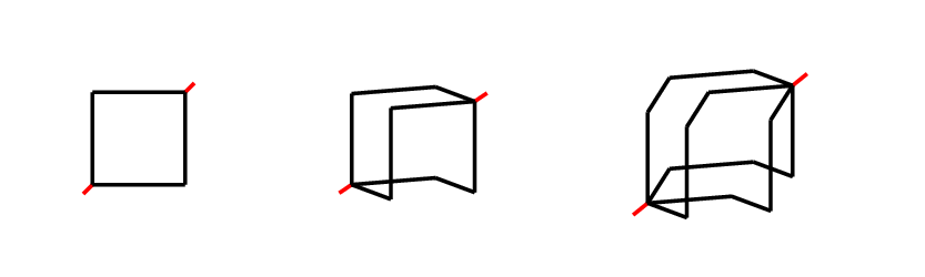
It remains to describe the hypercube gluing (recall that we are in the simplicial case). Let $C$ denote the $1$-skeleton of the $d$-dimensional cube, and with each edge of length $\lambda/d$. Let $e_{1},\cdots,e_{d}$ denote vectors of length $\lambda/d$ aligned positively along the $d$ coordinate axes in order. There is a path of length $\lambda$ from the vertex $(0,0,\cdots,0)$ to the vertex $(\lambda/d,\lambda/d,\cdots,\lambda/d)$ of $C$, obtained by concatenating straight segments of length $\lambda/d$ in the order $e_{1},e_{2},\cdots,e_{d}$. Taking $d$ cyclic permutations of this sequence of paths gives $d$ paths of length $\lambda$ between extremal vertices of $C$, whose union is a beachball. This is illustrated in Figure 10 in dimensions 2, 3 and 4.

There are $2^{d-1}$ pairs of extremal vertices of $C$, and the union of $2^{d-1}$ suitably labeled beachballs can be arranged along the $1$-skeleton of $C$ as above. Gluing the beachballs in this pattern is legal, and the resulting graph locally satisfies the first three conditions to be a $(m,d)$-regular simplicial spine.

The analog of the hypercube gluing for cubical spines is the lens gluing. This is the most complicated move in our construction, and we first describe this move in low dimensions before giving the definition in generality.

In dimension $2$ a beachball has degree 2 (i.e. it has 2 edges); $BC_{1}=\mathbb{Z}/2\mathbb{Z}$ acts as the full permutation group. Two beachballs with suitable labels can be identified along their boundaries, laid out along a circle; see Figure 11.

In dimension $3$ a beachball has degree 4; $BC_{2}=D_{4}$ acts by the dihedral group, preserving or reversing a circular order on the 4 edges. Eight beachballs with suitable labels can be glued up along a $K_{4,4}$ graph in $S^{3}$, where each edge of each beachball runs along a segment of length $2$ in the $K_{4,4}$ graph, as in Figure 12 (where one of the vertices is at “infinity” in the figure):

The lens gluing in dimension $d$ is closely related to the hypercube gluing in dimension $d-1$. Recall the definition of the hypercube gluing move from § 4.4. In this move, $2^{d-2}$ beachballs of degree $d-1$ are draped along the 1-skeleton of a $d-1$-dimensional cube; each edge of each beachball is subdivided into $d-1$ segments which run between antipodal vertices of the cube. We let $C$ denote the 1-skeleton of the cube, and denote the immersion of a beachball $b$ into $C$ by $b\to C$.

For any graph $L$, the spherical graph associated to $L$ is the graph with one $S^{0}$ (i.e. two vertices) for each vertex in $L$, and one $S^{0}*S^{0}$ for each edge in $L$. If $v$ is a vertex of $L$, we denote the corresponding pair of vertices in $S(L)$ by $v0$ and $v1$. Similarly, if $e$ is an edge of $L$, we denote the corresponding edges in $S(L)$ by $e00$, $e01$, $e10$ and $e11$ (in fact this construction generalizes in an obvious way to simplicial complexes of arbitrary dimension). There is a canonical simplicial map from $S(L)\to L$ which forgets the $01$ labels.

Now we apply this construction to $C$; the lens gluing will map $4\times 2^{d-2}$ beachballs of degree $2(d-1)$ into $S(C)$ in such a way that the projection to $C$ will map each 4 beachballs onto each degree $(d-1)$ beachball mapping into $C$ in the hypercube gluing, with each edge of the beachball downstairs in the image of two edges upstairs.

If $b\to C$ is a beachball, and $b^{\prime}\to S(C)$ is one of the four beachballs upstairs mapping to it, each edge of $b$ maps to a path in $C$ of length $d-1$, which is covered by two paths in $S(C)$ of length $d-1$. Each such path is determined (given its image in $C$) by a word of length $d$ in the alphabet $0,1$. Our beachballs upstairs have the property that the pair of lifts of each edge of $b$ are described by the same pair of $01$ words. Moreover, the collection of 4 pairs of $01$ words describing the lifts of $b$ are the same for all $b\to C$. So to describe the lens move we just need to give 4 sets of pairs of $01$ words of length $d$. We call these height pairs. An explicit formula for $d>2$ is given by

where $x$ is $0$ or $1$ depending on the parity of $d$, and where an expression like $w^{p/q}$ for $w$ a word of length $q$ means the initial string of length $p$ of the word $w^{\infty}:=www\cdots$. The meaning of this formula is best explained by a picture; see Figure 13.

The case $d=2$ is degenerate; the case $d=3$ gives rise to the height pairs

which reproduces four of the beachballs in the lens gluing for $d=3$ described above (the other four beachballs are in the preimage of the other beachball in the hypercube gluing).

Note that there is an ambiguity in our choice of labels of each pair of vertices of $S(C)$ over $v$ by $v0$ and $v1$; thus the group $\mathbb{Z}/2\mathbb{Z}^{\text{vert}(C)}$ acts by automorphisms of $S(C)$ over $C$. Thus although this is not evident in the formulae, under this symmetry group all four height pairs are in the same orbit.

The case $d=4$ is hard to draw without the diagram becoming cluttered; Figure 14 shows the 4 beachballs of degree 6 in the $d=4$ lens gluing which project to one beachball of degree 3 in the $d=3$ hypercube gluing.

The third condition for $(m,d)$-regularity is that each component of $L$ has exactly $m$ vertices which map to high-valent vertices of $\Sigma$. The only move which adjusts the number of such vertices on each component of $L$ is the elimination move. This move takes pieces which may be drawn from any component $L$; so we simply take enough disjoint copies of $L$, and symmetrize the components from which the moves are drawn, so that we apply this move the same number of times to every component. This will ensure the third condition for $(m,d)$-regularity.

The cocycle is sensitive to more combinatorial data than we have been using so far; it depends not only on the set of labels appearing as the edges in a beachball, but the way in which these labels come from consecutive even segments on each of ${\mathfrak{d}}$ blocks in a compatible ${\mathfrak{d}}$-tuple. Gluing different compatible ${\mathfrak{d}}$-tuples gives rise to the same beachball collections but with different cocycles (relative to a trivialization along the odd segments of the blocks). If the original gluing was done randomly, there are pairs of compatible segments whose gluings give rise to the same set of beachballs, but with cocycles differing by any element in the symmetric group $S_{d-1}$ in the simplicial case, or any element of $BC_{d-1}$ in the cubical case; adjusting the gluing by interchanging elements of these pairs gives the same collection of beachballs and the same remainder (and therefore the same gluing problem) but with the cocycle adjusted in the desired away. Boundedly many moves of this kind for each component produces an $(m,d)$-regular simplicial or cubical spine with all topological edges of length at least $\lambda$.

We now indicate how to modify our arguments and constructions so that they hold without our simplifying assumptions.

The first assumption — that the length $n$ of the relators is divisible by some big fixed constant $\lambda\cdot N$ (where also ${\mathfrak{d}}$ divides $\lambda$) — is easy to dispense with. We let $\rho$ be the remainder when dividing $n$ by $\lambda\cdot N$, then find ${\mathfrak{d}}$ copies of a subword of $r$ of length $\lambda\cdot N+\rho$ so that it is legal to glue these ${\mathfrak{d}}$ words in ${\mathfrak{d}}$ distinct copies of $r$; what is left after this step is a graph with edges whose lengths are divisible by $\lambda\cdot N$, and the rest of the construction can go through as before.

The second assumption — that the number $k$ of free generators satisfies $2k-1\geq 2d+1$ — can be finessed by looking more carefully at the construction. It can be verified that we do not really use the hypothesis that the word $r$ is random with respect to the uniform measure on reduced words of length $n$; instead we can make do with a much a weaker hypothesis, namely that we generate random words by any stationary ergodic Markov process, whose subword distribution of any fixed length has enough symmetry, and such that there are at least ${\mathfrak{d}}+1$ letters that may follow any legal substring.

The relevance of this is as follows: a random reduced word of length $n$ in a free group of rank $k$ can be thought of as a random reduced word of length $n/s$ in a free group of rank $k(2k-1)^{s-1}$ (whose symmetric generating set is the set of reduced words in $F_{k}$ of length $s$) generated by a certain stationary ergodic Markov process. We can perform matching of subwords and build spines in this new “alphabet”; the result will not immerse in $X$, since there might be folding of subtrees of diameter at most $2s$. But the spine will still have the crucial properties that the fundamental group of the 2-complex $\overline{M}$ is commensurable with $\Delta(m,d)$, and that the number of immersed paths of length $\nu$ grows like $(2k-1)^{s\nu/\lambda}$ where $\lambda$ is as big as we like. Taking $s$ big enough to “simulate” a group of rank at least $d+1$, we can then take $\lambda$ much bigger so that $s/\lambda$ is arbitrarily small. This small exponential growth rate of subpaths is the key to proving that $\pi_{1}(\overline{M})$ maps injectively with quasiconvex image.

The remainder of the argument is almost indentical to the arguments in [2] and [3], and makes use in the same way of the mesoscopic small cancellation theory for random groups developed by Ollivier [5]. It depends on two ingredients:

1. (1)

   a bead decomposition, exactly analogous to that in [2], § 5 or [3], § 4; and

2. (2)

   a mesoscopic small cancellation argument, which applies techniques of Ollivier as in [2], § 6 or [3], § 6.

We very briefly summarize the argument below just to indicate that no new ideas are needed, but refer the reader to the cited references for details.

A bead decomposition is an $(m,d)$-regular simplicial or cubical spine $\Sigma$ which is made up of $O(n^{\delta})$ pieces of size $O(n^{1-\delta})$ arranged in a circle, with each piece separated from the next by a neck (an unusually long glued segment) of length $C\log{n}$. We can construct a spine as in [3], § 4 as follows. Fix some small positive constant $\delta$ and write $r$ as a product

where each $r_{i}$ has length approximately $n^{1-\delta}$ and each $s_{i}$ has length approximately $n^{\delta}$, and we choose lengths so that $m$ is divisible by ${\mathfrak{d}}$. We then fix a small positive constant $C<\delta/\log(2k-1)$ and look for a common subword $x$ of length $C\log{n}$ in $s_{i},s_{i+m/{\mathfrak{d}}},\cdots,s_{i+({\mathfrak{d}}-1)m/{\mathfrak{d}}}$ with indices taken mod $m$, and then glue these distinct copies of $x$ into unusually long segments (called lips) of what will become the spine $\Sigma$.

The lips partition the remainder of $L$ into subsets $b_{i}$ each with mass $O(n^{1-\delta})$, and we can extend the partial gluing along the lips into an $(m,d)$-regular simplicial or cubical spine by gluing intervals in each $b_{i}$ independently. As in [2], § 5 and [3], § 4 the resulting spine $\Sigma$ has the property that for any positive $\beta$, any immersed segment $\gamma\to\Sigma$ with length $\beta n$ whose image in $X$ lifts to $r$ or $r^{-1}$, already lifts to $L$ (i.e. it appears in the boundary of a disk of $\overline{M}$). From this and the fact that a random 1-relator group is $C^{\prime}(\mu)$ for any positive $\mu$ it follows that $\overline{M}\to K_{r}$ is $\pi_{1}$-injective and its image is quasiconvex.

Finally, the fact that the valence of $\Sigma$ is uniformly bounded and the length of every segment is at least $\lambda$ where we may choose $\lambda$ as big as we like, implies that $\overline{M}\to K_{r}$ stays $\pi_{1}$-injective and quasiconvex when we attach the disks corresponding to the remaining $(2k-1)^{nD}-1$ random relations. This depends on Ollivier’s mesoscopic small cancellation theory [5]; the argument is exactly the same as that in [2], § 6 and [3], § 6.

This completes the proof of the Superideal Simplex Theorem and Superideal Cube Theorem.

References

- [1] I. Agol, The virtual Haken conjecture, With an appendix by Agol, Daniel Groves, and Jason Manning. Doc. Math. 18 (2013), 1045–1087
- [2] D. Calegari and A. Walker, Random groups contain surface subgroups, Jour. AMS 28 (2015), 383–419
- [3] D. Calegari and H. Wilton, 3-manifolds everywhere, preprint; arXiv:1404.7043
- [4] M. Gromov, Asymptotic invariants of infinite groups, Geometric group theory, vol. 2; LMS Lecture Notes 182 (Niblo and Roller eds.) Cambridge University Press, Cambridge, 1993
- [5] Y. Ollivier, Some small cancellation properties of random groups, Internat. J. Algebra Comput. 17 (2007), no. 1, 37–51
- [6] Y. Ollivier and D. Wise, Cubulating random groups at density less than , Trans. AMS 363 (2011), no. 9, 4701–4733
- [7] D. Wise, The structure of groups with a quasiconvex hierarchy, preprint.