Wave functions of pure gauge glueballs on the lattice
Abstract
The Bethe-Salpeter wave functions of pure gauge glueballs are revisited in this study. The ground and the first excited states of the scalar and tensor glueballs are identified unambiguously through the variational method. We calculate the wave functions in the Coulomb gauge and use two lattice spacings to check the discretization artifacts. For the ground states, the radial wave functions are approximately Gaussian and the size of the tensor glueball is roughly twice as large as that of the scalar glueball. For the first excited states, the radial nodes are clearly observed for both the scalar and the tensor glueballs, such that they can be interpreted as the first radial excitations. These observations may shed light on the theoretical understanding of the inner structure of glueballs.
pacs
11.15.Ha, 12.38.Gc, 12.39.MkI introduction
In quantum chromodynamics (QCD), gluons have strong interactions with each other and can form a new type of hadron, the glueball, which is distinct from the conventional mesons in the picture of the quark model. However, there is not yet a reliable theoretical description of the intrinsic degrees of freedom of glueballs. Phenomenologically, two-gluon glueballs are the simplest low-energy color singlet systems made up of gluons, whose quantum numbers are expected to be , , , etc. ( quantum number does not appear for two-gluon glueballs if the constituent gluons are massless). These arguments are in qualitative agreement with the pattern of the glueball spectrum obtained by lattice QCD calculations [1, 2, 3, 4], where the lowest-lying states are , , glueballs in the order of mass from low to high. As for the gluon dynamics inside glueballs, there are various effective approaches such as the bag model [5], QCD in Coulomb gauge [6, 7], and potential models [8, 9, 10]. The potential models depict a glueball as a bound state of two or more constituent gluons through a confining interacting potential. Even though still controversial, the potential models with proper theoretical assumptions can reproduce the glueball spectrum from lattice QCD.
Apart from the spectrum, some other static properties of glueballs, such as the Bethe-Salpeter (BS) wave functions, can also be investigated through lattice QCD studies, from which one can infer some qualitative information on the sizes and the spatial profiles of glueballs. For a glueball dominated by a two-gluon component, the BS wave function is defined through the matrix element of a two-gluon operator between the glueball state and the vacuum, which can be derived from the relevant two-point function calculated in lattice QCD. This kind of wave function may reflect the spatial structure of a hadron to some extent. Since the two-gluon operator is obviously gauge variant, the related calculation should be performed in a fixed gauge, for example, the Coulomb gauge. The pioneering study on this topic was carried out for the pure gauge glueballs [11]. A similar study on glueballs can be found in Ref. [12].
There are actually phenomenological studies [13, 14] on the gluon dynamics within glueballs by the use of the BS wave functions obtained from lattice QCD calculations, where the positive C-parity states are taken as mainly two-gluon states and the interacting potential between the constituent gluons is extracted. However, the previous lattice studies focus only on ground states and the results are not precise enough, thus a more scrutinized analysis is desired for the BS wave functions of both the ground and the excited states. This is exactly the major goal of this work. It is known that the key point in the calculation of the matrix elements mentioned above is to identify the glueball states unambiguously. In order for this, we adopt the sophisticated technique used in the glueball spectrum study [1, 2, 3]. This technique implements the variational method based on large operator sets for glueballs, through which the ground and the first excited states can be well determined. Finally, the BS wave functions of all the glueball states are derived to a high precision. We hope our results can provide more information to the understanding of the nature of glueballs.
This paper is organized as follows. Section II gives a detailed introduction to the definition of two-gluon operators on the lattice. Section III contains the numerical details in calculating the BS wave functions. In Section III we also discuss the parameterizations of the wave functions and the corresponding physical implications. A brief summary is given in Section IV.
II Two-gluon operators
It is known that the Bethe-Salpeter equation [15] provides a relativistic description of a two-body system where the relativistic Bethe-Salpeter (BS) wave function of a bound state can then be defined. For a two-gluon glueball state in its rest frame, the BS wave function can be expressed as [11]:
| (1) |
where stands for the spatial orientation of , the summations on and guarantee the right quantum number of the state , and the gauge field acts as the creation operator for a gluon. Since the fundamental gluonic variables on the lattice are the gauge links instead of , one has to build the lattice counterpart of the two-gluon operator through gauge links .
The gauge field can be directly defined as
| (2) |
by the use of the relations
| (3) |
and the classical small- expansion of . The two-gluon operator through this way is denoted as in this work. In Ref. [11] the authors propose an alternative definition of the two-gluon operators (denoted as )
and claim that this definition reduces the possible mixing with the flux states. Although flux states do not appear in this work (see below), we also carry out the relevant calculation using to check the possible lattice artifacts owing to the different definitions of the two-gluon operators.
However, the classical expansion of is not very justified due to the tadpole diagrams if the quantum effects are considered. In view of this fact, we propose an alternative way to define from through a non-linear derivation,
| (4) |
For any , which is an element of the group, there exists an unitary matrix satisfying
| (5) |
with , being the 3 eigenvalues of the matrix . Thus Eq. (4) can be solved exactly as
| (6) |
The subsequent two-gluon operators are called in this work.
The spatial symmetry group on a lattice is the discrete octahedral point group instead of the group in the continuum limit, whose irreducible representations are . Although the correspondences of these irreducible representations to the angular momenta are not unique, it is always conjectured that the lowest states in each symmetry channel correspond to the states with lowest ’s in the continuum. To be specific, the quantum number of the scalar glueball () is realized by the irreducible representation on the lattice, and that of the tensor glueball is given by both and . The two-gluon operators belong to the above irreducible representatives are expressed explicitly as
| (7) |
where the s with the same and different spatial orientations are summed up and the variable is omitted for convenience.
III Numerical details
We generate the gauge configurations on two anisotropic lattices using the tadpole-improved gauge action [1]. The lattice sizes are and , respectively. The temporal lattice spacing is made much smaller than the spatial one with the anisotropy . Thus we can obtain a higher resolution of hadron correlation functions in the temporal direction, which helps us to handle glueball states whose signal-to-noise ratios damp rapidly in time. The relevant input parameters are listed in Tab. 1, where the values are determined through the static potential with the scale parameter . There are 5000 gauge configurations generated for each lattice. The volumes of both lattices are roughly , which have been tested to be large enough for glueballs [3].
| (fm) | (fm) | |||||
|---|---|---|---|---|---|---|
| 2.4 | 5 | 0.461(4) | 0.222(2)(11) | 5000 | ||
| 2.8 | 5 | 0.288(2) | 0.138(1)(7) | 5000 |
The BS wave function in the rest frame of a glueball state can be derived by calculating the following two-point functions of the two-gluon operator defined above and an operator which creates glueball states with a specific quantum number,
| (8) | |||||
where is the mass of the -th state, and is its BS wave function by the definition of Eq. (1) (up to an irrelevant normalization factor). Since the two-gluon operators are gauge variant objects, we need to calculate the two-point functions in a fixed gauge. In the practical calculation, all the gauge configurations are fixed to the Coulomb gauge, in which the BS wave functions are usually assumed to have connection with the wave functions of potential models.
In this work we intend to obtain the wave functions of both the ground and the first excited glueball states, so the major task is to identify a specific state unambiguously. For this purpose, we adopt the techniques applied in the calculation of the glueball spectrum to construct the optimal glueball operators which couple to specific states. Subsequently, we use as the operator in Eq. (8) to calculate the required correlation functions. It should be noted that, with this prescription, the possible mixing of glueballs to the flux states [11] can be eliminated, or at least much suppressed by the use of the optimal operators. We outline the construction of as follows.
As is mentioned above, the quantum numbers of glueballs are realized through the irreducible representations , , , , and of the lattice point group . Therefore, we first build the same 10 prototypes of Wilson loops as those in Refs. [2, 3], based on which several smearing steps are applied to obtain more loop operators for glueballs. We perform the 24 spatial operations of the group to these operators and linearly combine them to realize the irreducible representations of , and . As such we obtain 24 different operators for each of the quantum numbers , or . Finally, we implement the variational method to get the optimal operators by solving the generalized eigenvalue problem. To be specific, for a given quantum number , we first calculate the correlation matrix through the operator set ,
| (9) |
and then solve the generalized eigenvalue problem
| (10) |
to obtain the eigenvector for the -th eigenvalue . In this work we choose . The eigenvector yields the combination coefficients for the optimal operator,
| (11) |
It has been verified in the calculation of the spectrum that is highly optimized and its correlation function is saturated by the -th state even at the beginning time slice. In other words, the correlation function of can be consequently expressed as
| (12) |
where is normalized as , and is the mass of the state.

| (GeV) | (GeV) | (GeV) | (GeV) | (GeV) | (GeV) | |
|---|---|---|---|---|---|---|
| 2.4 | 1.36(1)(7) | 2.58(4)(13) | 2.40(4)(12) | 3.29(13)(16) | 2.36(4)(12) | 3.34(13)(16) |
| 2.8 | 1.52(2)(8) | 2.92(20)(15) | 2.31(4)(11) | 3.42(15)(17) | 2.31(3)(11) | 3.49(21)(17) |
The effective mass plateaus of the ground and the first excited states of scalar and tensor glueballs are plotted in Fig. 1, where one can see that the effective mass plateau in each channel starts almost from the first time slice. The masses of the ground and the first excited glueball states in the , , and channels are given in Tab. 2 in physical units, which are converted through the scale parameter MeV. It is also seen that the masses of the glueballs have obvious lattice spacing dependence, while the masses of the and glueballs are insensitive to the lattice spacings. Our results are consistent with that of the previous studies [2, 3]. The coincidence of the masses of and glueballs at the same lattice spacing implies that the effects due to the rotational symmetry breaking are not important on the lattices we are using.
By using the optimal glueball operators, the two-point function can be simplified as
| (13) |
where is the mass of the glueball state in concern, is an irrelevant normalization factor, and is the desired wave function. Consequently, can be directly obtained through a single-exponential fit. For a definite state, since the mass is a common parameter of the two-point functions with different s as well as the relevant , we perform a joint data analysis on these correlation functions. We first divide the 5000 measurements of the two-point functions into 100 bins and take the average of the 50 measurements in each bin as an independent measurement. After that we construct a bootstrapped covariance matrix of these correlation and carry out a correlated minimal- data fitting, through which the wave functions at different s can be obtained simultaneously . For all the channels we are interested in, the fitting qualities are very good.
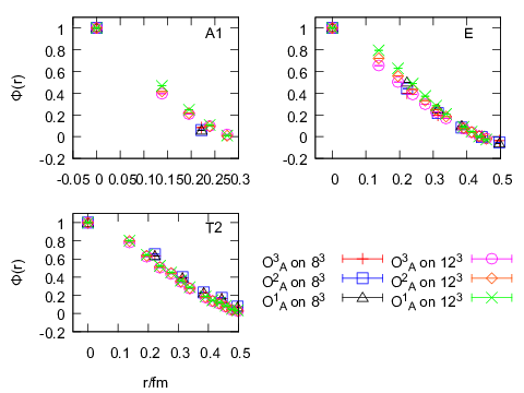
We first test the three definitions of the two-gluon operators on the two lattices we are using. The ground state wave functions in the , , and channels are plotted in Fig. 2 for comparison, where the spatial distances are expressed in physical units based on the lattice spacings listed in Tab. 1. In each channel, the wave functions from the three types of the two-gluon operators lie on the same curve within errors. This implies that the three definitions of the two-gluon operators are numerically equivalent. On the other hand, the wave functions from the two lattices do not show sizable difference and manifest that the finite artifacts are not important. This observation is understandable since we are using the improved action, which suppresses the discretization error substantially. Therefore, in the following data analysis and discussions in this paper, we focus only on the wave functions derived from the finer lattice with the third definition of the two-gluon operators.
| (fm) | |||
|---|---|---|---|
| (fm) |

In order to get some quantitative information, we parameterize the ground state wave functions as the following function form,
| (14) |
where the parameters and can be determined by fitting the lattice data. Since the measured values of the wave functions at different are correlated, in extracting and we perform the correlated data fitting with a bootstrapped covariance matrix. The best-fit results are listed in Tab. 3 for the three channels on the lattice. It is interesting that the parameter is close to 2 within errors for all the cases. This is very different from the previous work [11, 12] where is Coulomb type instead of the Gaussian type in this study. The fitted wave functions of the ground states for the three channels are plotted in Fig. 3 for illustration. It should be noted that the wave functions of and ground state glueballs are slightly different, which can be attributed to the rotational symmetry breaking on the lattice. Obviously, the effect of this kind of symmetry breaking is enlarged in the spatially extended quantities such as the wave functions, even though their masses are nearly degenerate.
We also calculate the root-of-mean-square (RMS) radii for the ground state glueballs with the definition
| (15) |
where is the wave function with the best-fit parameters. The results are also listed in Tab. 3. The ’s of the and glueballs are almost twice as large as that of the glueball.

| (fm) |
|---|
Benefiting from the variational method discussed above, we can also identify clearly the first excited states of glueballs in the three channels. This enables us to derive their wave functions as well, and the procedure is similar to that for the ground states. Fig. 4 (the points) shows the wave functions of the , and excited glueballs. We do observe the radial nodes for all these wave functions, which can be viewed as a strong evidence that the excited glueball is the first radial excited state of the ground glueball in each channel. Inspired by the function form of the two-body non-relativistic Schrödinger equation, we parameterize the wave functions of the first excited states as follows,
| (16) |
where the parameter depends on the type of the interacting potential (for example, for the Coulomb potential and for the harmonious oscillator potential). The parameters , , and are determined through a procedure similar to that for the ground states, and the best-fit results for the lattice are listed in Tab. 4. It is interesting that and in the tensor channel ( and ) are close to those of the ground state. Especially, is still close to 2, which resembles the case for the harmonious oscillator potential model. For the first excited state of the scalar glueball, the fitted parameter deviates from 2 a little. The reason for this is not clear yet. Recalling that the size of ground scalar glueball is as small as 0.127 fm, while the lattice spacings we are using are comparable to it or even larger, so a possibility is that the radial behavior of the first excited scalar glueball is not extracted accurately enough.
IV Summary and Discussions
The Bethe-Salpeter wave functions of the pure gauge scalar and tensor glueballs are revisited in this work. The feature of this study is the precise identification of the ground and the first excited glueball states in these two channels through the variational method based on large operator sets. We test the different definitions of two-gluon operators and find no sizable difference, which implies the finite lattice spacing artifacts are small due to the implementation of the improved gauge action. This is also reinforced by checking the results from two lattices with different lattice spacings.
With large statistics, the BS wave functions of both the ground and the first excited states in the scalar and tensor channels are extracted precisely. Instead of the exponential fall-off of the wave functions observed in previous works, we find that the wave functions of the ground states are Gaussian-like. The size of the ground state tensor glueball is roughly twice as large as that of the ground state scalar glueball. For the first time, we observe the radial nodes of wave functions of the first excited states, which support them as the first radial excitations. We use the function forms inspired by potential models to parameterize the wave functions, and the fitted parameters show that the wave functions of the ground and the first excited state in the tensor channel are compatible with the and wave functions of a harmonious oscillator. These observations are helpful for a qualitative understanding of the inner structure of glueballs. Furthermore, there have been quite a few phenomenological studies on glueballs in the picture of potential models [17, 14, 13, 16], which use the scalar glueball wave function as an input to derive the interacting potential between constituent gluons. The results in this work can provide much finer and more precise information on this sector.
ACKNOWLEDGEMENTS
This work is supported in part by the National Science Foundation of China (NSFC) under Grants No. 10835002, No. 11075167, No. 11105153, No. 11335001, and 11405053. Z.L. is partially supported by the Youth Innovation Promotion Association of CAS. Y.C. and Z.L. also acknowledge the support of NSFC under No. 11261130311 (CRC 110 by DFG and NSFC)
References
- [1] C. Morningstar and M. Peardon, Phys. Rev. D 56, 4043 (1997).
- [2] C. Morningstar and M. Peardon, Phys. Rev. D 60, 034509 (1999).
- [3] Y. Chen et al., Phys. Rev. D 73, 014516 (2006).
- [4] E. Gregory, A. Irving, B. Lucini, C. McNeile, A. Rago, C. Richards, and E. Rinaldi, J. High Energy Phys. 10 (2012) 170.
- [5] C.E. Carlson, T.H. Hansson, C. Peterson, Phys. Rev. D 27, 1556 (1983).
- [6] A. Szczepaniak, E.S. Swanson, C.-R. Ji, S.R. Cotanch, Phys. Rev. Lett. 76, 2011(1996) [arXiv:hep-ph/9511422].
- [7] A. Szczepaniak, E.S. Swanson, Phys. Lett. B 577, 61 (2003) [arXiv:hep-ph/0308268].
- [8] H. Fritzsch, P. Minkowski, Nuovo Cimento A 30, 393 (1975).
- [9] T. Barnes, Z.Phys. C 10, 275 (1981).
- [10] J.M. Cornwall, A. Soni, Phys. Lett. B 120, 431 (1983).
- [11] P. de Forcrand and K.-F. Liu, Phys. Rev. Lett. 69, 245 (1992).
- [12] M. Loan and Y. Ying, Prog. Theor. Phys. 116, 169 (2006).
- [13] F. Buisseret and C. Semay, Eur. Phys. J. A 33, 87 (2007).
- [14] F. Buisseret, Phys. Rev. D 79, 037503 (2009).
- [15] E.E. Salpeter, H.A. Bethe, Phys. Rev. 84, 1232 91951); J. Schwinger, Proc. Natl. Acad. Sci. U.S.A. 37, 455 (1951).
- [16] N. Boulanger, F. Buisseret, V. Mathieu, and C. Semay, Eur. Phys. J. A 38, 317 (2008).
- [17] V. Mathieu, F. Buisseret, and C. Semay, Phys. Rev. D 77, 114022 (2008).