A Structure Preserving Scheme for the Kolmogorov-Fokker-Planck Equation

Erich L Foster¹¹ 1 Basque Center for Applied Mathematics, 48009 Bilbao, Basque Country - Spain (efoster@bcamath.org, tbinh@bcamath.org). Jérôme Lohéac²² 2 LUNAM Université, IRCCyN UMR CNRS 6597 (Institut de Recherche en Communications et Cybernétique de Nantes), École des Mines de Nantes, 4 rue Alfred Kastler, 44307 Nantes - France (Jerome.Loheac@irccyn.ec-nantes.fr) and Minh-Binh Tran¹¹ 1 Basque Center for Applied Mathematics, 48009 Bilbao, Basque Country - Spain (efoster@bcamath.org, tbinh@bcamath.org).

August 24, 2026

Abstract

In this paper we introduce a numerical scheme which preserves the long time behavior of solutions to the Kolmogorov equation. The method presented is based on a self-similar change of variables technique to transform the Kolmogorov equation into a new form, such that the problem of designing structure preserving schemes, for the original equation, amounts to building a standard scheme for the transformed equation. We also present an analysis for the operator splitting technique for the self-similar method and numerical results for the described scheme.

keywords

Kolmogorov equation, long time asymptotic, structure preserving scheme, self-similarity

AMS

65M12, 65M22, 35K65

1 Introduction

In this paper, we are interested in the following Kolmogorov-Fokker-Planck equation

\partial_{t}f-\partial_{v}^{2}f-v\partial_{x}f=0.

(1)

As can see from its form, the solution of the equation does not only diffuse in the direction of $v$ , by the effect of the diffusion operator $\partial_{v}^{2}$ , but it is also diffuses in the direction of $x$ , due to the transport equation $\partial_{t}f-v\,\partial_{x}f$ . The hypoellipticity and the asymptotic behavior of this operator is well known, see for instance the original work of L. Hörmander [17] and the work of C. Villani [27] and F. Rossi [24]. The solution to the Kolmogorov equation is known to decay polynomially in time, and it is our goal to preserve this decay rate through numerical schemes.

To our knowledge, only a few papers investigate this large time asymptotic of numerical solutions of Fokker-Planck type equations. One of most popular schemes for Fokker-Planck equations of the type

\partial_{t}u(x)=\frac{1}{M(x)}\mbox{div}(N(x)\nabla u(x)+P(x)u(x)),

(2)

is the Chang and Cooper method [9], which is a finite difference scheme in both space and time directions. The Chang Cooper method has been developed later in [6] and [23]. In [3], [4] and [8], the authors studied nonlinear Fokker-Planck equations, where the nonlinearity enters into the diffusion. Systems of Fokker-Planck type equations have also been studied in [12] and [16] by a Voronoi finite volume discretization. However, most of the equations studied before posses full parabolic strutures, and thus the existing approaches could not be applied to the Kolmogorov equation, which has a different structure: there is an advection but no diffusion term in the $x$ variable.

It is our aim to introduce a new method based on a self-similar technique to obtain a satisfying long time behavior for numerical solutions of equations with hypocoercive structures. Since the Kolmogorov equation is highly convective, one might expect stability issues, thus a natural approach to solve the Kolmogorov equation numerically is to use an operator splitting technique, where the Kolmogorov equation is splitted into two equations: a transport and a heat equation. Like the heat equation the Kolmogorov equation contains a diffusion operator and so some behaviors from the heat equation can also be observed in the Kolmogorov equation. In order to solve the heat equation by some discretization method, one needs to restrict the domain $\mathbb{R}^{2}$ to a bounded domain and impose boundaries condition. However, it is known that the support of the solution to the heat equation spreads to the whole space as time evolves, therefore restricting the computational domain to a bounded domain is not an ideal strategy, if we want to observe the long time behavior of the solution (1).

Another approach is to perform the change of variables

f(t,v,x)=g(t,v,x+t\,v)=g(t,v,z),

(3)

then (1) becomes

\partial_{t}g=\partial_{v}^{2}g+2t\,\partial_{vz}g+t^{2}\partial_{z}^{2}g.

(4)

Since the frame of reference follows the transport we no longer have an issue with stability and thus one can apply a method such as the finite element method (FEM) without much problem. However, the problem, again, is we need to restrict the computational domain to a bounded domain, while the support of the solution of the equation spreads to the whole space as time evolves. In § 4.1, we prove that for a truncated domain, the solutions of (1) and (4) set in a bonded domain with homogeneous Dirichlet boundary conditions converge exponentially to $0$ , while for the original Cauchy problem the convergence is expected to be polynomial.

Inspired by the self-similarity technique in control theory (see, for instance, [10, 11]), we propose, in Section 3, a new strategy to design structure preserving schemes for the Kolmogorov equation by using the technique of self-similarity change of variables. Thus, we see simulations are more computationally efficient and less reliant on artificial boundary conditions. By the self-similarity technique, we transform Kolmogorov equation into the following equation:

\partial_{s}\widetilde{g}=2(1-e^{-s})\partial_{\widetilde{v}\widetilde{z}}\widetilde{g}+\partial_{\widetilde{v}}^{2}\widetilde{g}+(1-e^{-s})^{2}\partial_{\widetilde{z}\widetilde{z}}\widetilde{g}+\frac{1}{2}\widetilde{v}\partial_{\widetilde{v}}\widetilde{g}+\frac{3}{2}\widetilde{z}\partial_{\widetilde{z}}\widetilde{g}+2\widetilde{g}.

(5)

Therefore, problem of designing schemes preserving asymptotic behavior for the Kolmogorov equation becomes a problem of designing a standard scheme for the determining the solution, $\widetilde{g}$ , to (5). Then on this new problem the numerical study of the convergence rate will be more easy, since the convergence rate in the original variables will be preserved if the self-similar solution is converge to a steady state. Consequently, numerically speaking we have to check weather the self-similar solution converges to a steady state. This fact appears to be true for a classical finite element method as on can chek on figures 5 and 2b.

We prove in Proposition 4 and Theorem 5 that the behavior of the $L^{\infty}$ norm of $\widetilde{g}$ convergence to a steady state as time tends to infinity. We then introduce Algorithm 2 as a way to discretize (5) by an operator splitting technique combined with a finite element method where the domain is truncated into a bounded one. We prove the convergence of the truncated method and the analysis of the operator splitting technique in Proposition 7, Theorem 9 and Corollary 10. In (13), we represent a condition that the truncated domain should satisfy in order to guarantee the convergence to the steady state of the self-similar solution. We also provide numerical simulations to illustrate our self-similarity technique. Numerically, the self-similarity technique has a major benefit, in that, for long time simulation one need not choose a large domain, since the solution maintains compact support for a well chosen initial domain. Additionally, the time scaling allows for fast time marching and so simulations are more computationally efficient and less reliant on artificial boundary conditions. Thus, the main benefits of using a self-similar change of variables include: small space domain, and fast marching in time. In Section 5 we demonstrate these properties by comparing the numerical simulations of the Kolmogorov equation in its original form, in its Lagrangian variable form, and in its self-similarity form. We demonstrate that not only is the self-similarity change of variable more computationally efficient in the sense of computational resources used, but also in the size of the error resulting from the numerical scheme used.

We would also like to mention a similar technique: In [14, 13], F. Filbet et al. introduce a new technique based on the idea of rescaling the kinetic equation according to hydrodynamic quantities. The rescaling in velocity, is as follows

f(t,x,v)=\frac{1}{\omega(t,x)^{d_{v}}}g\left(t,x,\frac{v}{\omega(t,x)}\right),

where the function $\omega$ is an accurate measure of the support of the function $f$ . The rescaling can be defined based on the information provided by the hydrodynamic fields, computed from a macroscopic model corresponding to the original kinetic equation. However, the collisional kinetic equations considered by F. Filbet et al. are much more sophisticated than the Kolmogorov equation, since they are nonlinear. Therefore, the scaling in space $\omega(t,x)$ has to be computed through hydrodynamic quantities, while in our case, the space scale is quite simple to compute.

Our idea is quite similar to theirs, but goes further; we not only rescale the velocity variable, but also the time variable. Indeed, rescaling in time results in convergence to a steady state instead of either exponential or even polynomial decay. This has the benefit of maintaining compact support, rather than an expansion of the solution to the whole space. Numerically, one can see with the time rescaling, as time evolves, the support of the self-similarity solution is trapped in a bounded domain if the initial condition is compactly supported.

Remark 1.1.

Rescaling/self-similar algorithms are a well-known strategy in constructing numerical schemes, which can capture the profile of blow up solutions. Such algorithms were first introduced in [2] and have continued to be developed in [5, 22, 18, 25].

The structure of the paper is as follows: In Section 2, we recall some classical results on the kernel and asymptotic behavior of the solution of the Kolmogorov equation. In Section 3, we introduce the self similar formulation of the Kolmogorov equation. We also provide a theoretical study on the solution of the self similar equation: in Proposition 4 the solution is proven to be bounded and converges to a steady state in Theorem 5. In order to solve the Kolmogorov equation numerically, one needs to truncate the full space to a bounded domain, thus in Section 4 we introduce the methods for simulating the Kolmogorov equation in a bounded domain, including operator splitting methods for both the original form of the Kolmogorov equation and the Self-Similar form of the Kolmogorov equation. In § 4.1, we discuss truncating the domain for the Kolmogorov equation in three forms: the original form (1), the Lagrangian form (4) and the self-similar form (5). We prove that once the domain is truncated the solution to the the original form (1) and the Lagrangian form (4) converge exponentially to $0$ , which does not correspond to the polynomial convergence predicted for the original Cauchy problem. For the self-similar case (5), we will see numerically that the solution converges to a steady state. This coincides with the property of the original Cauchy problem. As a consequence, we choose to truncate and discretize the self-similar equation (5) by an operator splitting technique combined with a finite element method. The convergence of the truncated method and the analysis of the operator splitting technique is given in Proposition 7, Theorem 9 and Corollary 10. We also give a necessary condition, (13), wich should be satisfied for the troncated domain in order to obtain a time asymptotic convergence to a steady state. Furthermore, numerical results verifying the theory are presented in Section 5.

2 Kernel and Long Time Behavior

In this section we recall the kernel for the Kolmogorov equation on the whole space and describe the long term behavior. This will be useful in determining the correctness of the methods developed in later sections and for developing the self-similarity change of variables.

2.1 Kernel

In what follows, for the sake of completeness, we recall the kernel for the Kolmogorov equation. The kernel is obtained by a standard method using the Fourier transform. These results were originally obtained by A. Kolmogorov [20] in the sixties and a more general statement was developed by O. Calin, D.-C. Chang and H. Haitao [7] or in K. Beauchard and E. Zuazua [1].

Proposition 1.

The kernel of (4) is:

G_{t}(v,z)=\frac{\sqrt{3}}{2\pi t^{2}}e^{-\frac{1}{4\,t^{3}}(3z^{2}+(2t\,v-3z)^{2})}\qquad(t>0,\,x\in\mathbb{R},\,v\in\mathbb{R}),

(6)

Given an initial data, $f_{0}\in C^{\infty}(\mathbb{R}^{2})$ , the solution $f(t,v,x)$ to (1) is given by the convolution

f(t,v,x)=(f_{0}*G_{t})(v,x+v\,t)i\qquad(t>0,\,x\in\mathbb{R},\,v\in\mathbb{R}).

(7)

With the kernel for the Kolmogorov equation in hand we will be able to better understand the behavior of the Kolmogorov system, since the kernel allows one to compute the exact solution through a convolution. Additionally, knowing the behavior of the system will allow us to evaluate the validity of any numerical method applied to the Kolmogorov equation.

2.2 Long Time Behavior of the Kolmogorov Equation

In what follows, we will give some more precise decay rates, using the explicit form to the solution of (1) given in Proposition 1. Substituting $z=x+v\,t$ into (6) we see the kernel in $(v,x)$ variables is

G_{t}(v,x+v\,t)=\frac{\sqrt{3}}{2\pi t^{2}}e^{-\frac{1}{4\,t^{3}}(3\,(x+t\,v)^{2}+(3x+t\,v)^{2})}.

Thus, the kernel represents a series of ellipses given by the Gaussian

e^{-\frac{1}{4\,t^{3}}(3\,(x+t\,v)^{2}+(3x+t\,v)^{2})},

where the spread of the ellipse is described by the standard deviation $\frac{2t^{\frac{3}{2}}}{\sqrt{3}}$ in the direction $x+t\,v$ while the spread in the direction $3\,x+t\,v$ is described by the standard deviation $2\,t^{\frac{3}{2}}$ . Thus, we see not only that the shape changes over time, but the width of the solution changes over time, and it changes to a varying degree in different directions.

Now we want to know what the behavior of (1) is as $t\to\infty$ . It remains clear that $\lim_{t\to\infty}G_{t}(v,x)=0$ . But let us give a more precise asymptotic on $G$ .

Lemma 2.

For every $q\in[1,\infty]$ and every $t>0$ , we have $G_{t}\in L^{q}(\mathbb{R}^{2})$ and

\|G_{t}\|_{L^{q}(\mathbb{R}^{2})}=\begin{cases}q^{\frac{-1}{q}}\left(\dfrac{\sqrt{3}}{2\pi t^{2}}\right)^{\frac{q-1}{q}}&\text{if }q\in[1,\infty),\\[10.00002pt] \dfrac{\sqrt{3}}{2\pi t^{2}}&\text{if }q=\infty.\end{cases}\qquad(t>0).

Proof.

Let $G_{t}$ be the function defined in Proposition 1. Then for every $q>0$ , we have:

	$\displaystyle\\|G_{t}\\|_{L^{q}(\mathbb{R}^{2})}^{q}$	$\displaystyle=\left(\frac{\sqrt{3}}{2\pi t^{2}}\right)^{q}\int_{\mathbb{R}^{2}}\!\exp\left(\frac{-q}{4\,t^{3}}\left(3z^{2}+\left(2t,v-3z\right)^{2}\right)\right)\,dv\,dz$
		$\displaystyle=\frac{1}{2\sqrt{3}t}\left(\frac{\sqrt{3}}{2\pi t^{2}}\right)^{q}\int_{\mathbb{R}^{2}}\!\exp\left(\frac{-q}{4\,t^{3}}\left(w^{2}+u^{2}\right)\right)\,dw\,dz$
		$\displaystyle=\frac{1}{2\sqrt{3}t}\left(\frac{\sqrt{3}}{2\pi t^{2}}\right)^{q}\frac{4\pi t^{3}}{q}=\frac{3^{\frac{q-1}{2}}}{q(2\pi)^{q-1}}t^{-2(q-1)}.$

and the result in the $L^{\infty}$ is obvious. ∎

Corollary 3.

Let $p,q,r\in[1,\infty]$ such that $\frac{1}{p}+\frac{1}{q}=1+\frac{1}{r}$ .
If $f_{0}\in L^{p}(\mathbb{R}^{2})$ , then the solution $f$ of (1) satisfies for every $t>0$ , $f(t)\in L^{r}(\mathbb{R}^{2})$ , and

\|f(t)\|_{L^{r}(\mathbb{R}^{2})}\leqslant\begin{cases}\displaystyle{\frac{C(q)}{t^{2(1-\frac{1}{q})}}\|f_{0}\|_{L^{p}(\mathbb{R}^{2})}}&\text{if }q\in[1,\infty),\\[10.00002pt] \displaystyle{\frac{C(q)}{t^{2}}\|f_{0}\|_{L^{p}(\mathbb{R}^{2})}}&\text{if }q=\infty,\end{cases}

(8)

with $C(q)=q^{\frac{-1}{q}}\left(\frac{\sqrt{3}}{2\pi}\right)^{\frac{q-1}{q}}$ if $q\in[1,\infty)$ and $C(q)=\frac{\sqrt{3}}{2\pi}$ if $q=\infty$ .

Proof.

The proof of Corollary 3 follows directly from Young’s inequality and Lemma 2. ∎

3 Self-similar formulation of the Kolmogorov operator

In this section, we will present how we derive the self-similar form, (5), for the Kolmogoref equation, (1). In addition, we will prove the convergence of $\widetilde{g}$ , solution of (5), to a steady state as the time tends to infty. More other, we will also give quite surprizing remark establishing that the behavior of the norm of $\widetilde{g}$ is not motonous.

Let us introduce the function $g$ as in (3) to obtain (4). Now define the change of variables

\widetilde{g}(s,\widetilde{v},\widetilde{z})=e^{2s}g(e^{s}-1,e^{s/2}\widetilde{v},e^{3s/2}\widetilde{z})\qquad((s,\widetilde{v},\widetilde{z})\in\mathbb{R}_{+}\times\mathbb{R}\times\mathbb{R}),

then

	$\displaystyle\partial_{s}\widetilde{g}(s,\widetilde{v},\widetilde{z})$	$\displaystyle=e^{2s}\big[e^{s}\partial_{t}g(e^{s}-1,e^{s/2}\widetilde{v},e^{3s/2}\widetilde{z})+2g(e^{s}-1,e^{s/2}\widetilde{v},e^{3/2s})$
		$\displaystyle\quad+\frac{1}{2}e^{s/2}\widetilde{v}\,\partial_{v}g(e^{s}-1,e^{s/2}\widetilde{v},e^{3s/2}\widetilde{z})+\frac{3}{2}e^{3s/2}\widetilde{z}\,\partial_{z}g(e^{s}-1,e^{s/2}\widetilde{v},e^{3s/2}\widetilde{z})\big],$
	$\displaystyle\partial_{\widetilde{v}}\widetilde{g}(s,\widetilde{v},\widetilde{z})$	$\displaystyle=e^{5s/2}\partial_{v}g(e^{s}-1,e^{s/2}\widetilde{v},e^{3s/2}\widetilde{z}),~~~~~~~\partial_{\widetilde{z}}\widetilde{g}(s,\widetilde{v},\widetilde{z})=e^{7s/2}\partial_{z}g(e^{s}-1,e^{s/2}\widetilde{v},e^{3s/2}\widetilde{z}),$
	$\displaystyle\partial_{\widetilde{v}\widetilde{z}}\widetilde{g}(s,\widetilde{v},\widetilde{z})$	$\displaystyle=e^{4s}\partial_{vz}g(e^{s}-1,e^{s/2}\widetilde{v},e^{3s/2}\widetilde{z}),~~~~~~~~\partial_{\widetilde{v}}^{2}\widetilde{g}(s,\widetilde{v},\widetilde{z})=e^{3s}\partial_{vv}g(e^{s}-1,e^{s/2}\widetilde{v},e^{3s/2}\widetilde{z}),$
	$\displaystyle\partial_{\widetilde{z}}^{2}\widetilde{g}(s,\widetilde{v},\widetilde{z})$	$\displaystyle=e^{5s}\partial_{zz}g(e^{s}-1,e^{s/2}\widetilde{v},e^{3s/2}\widetilde{z}).$

After substituting the above into (4) and rearranging we get the following version of the Kolmogorov equation in self-similar variables


		$\displaystyle\partial_{s}\widetilde{g}=2(1-e^{-s})\partial_{\widetilde{v}\widetilde{z}}\widetilde{g}+\partial_{\widetilde{v}}^{2}\widetilde{g}+(1-e^{-s})^{2}\partial_{\widetilde{z}\widetilde{z}}\widetilde{g}+\frac{1}{2}\widetilde{v}\partial_{\widetilde{v}}\widetilde{g}+\frac{3}{2}\widetilde{z}\partial_{\widetilde{z}}\widetilde{g}+2\widetilde{g},$		(9a)
		$\displaystyle\widetilde{g}(0,\cdot,\cdot)=f_{0}.$		(9b)

Let us now give some qualitative behavior on $\widetilde{g}$ . More precisely, we will discuss the behavior of the norm of $\widetilde{g}$ . It is easy to see that:

\frac{1}{2}\frac{\partial\|\widetilde{g}(s)\|_{L^{2}(\mathbb{R}^{2})}^{2}}{\partial s}=-\left\|(1-e^{-s})\partial_{\widetilde{z}}\widetilde{g}(s)+\partial_{\widetilde{v}}\widetilde{g}(s)\right\|_{L^{2}(\mathbb{R}^{2})}^{2}+\left\|\widetilde{g}(s)\right\|_{L^{2}(\mathbb{R}^{2})}^{2}\qquad(s>0).

So we can see the evolution of the norm of $\widetilde{g}$ is the result of the competition between the norm of $\widetilde{g}$ and the norm of the ”divergence” of $\widetilde{g}$ . But since we are working on an unbounded domain, we cannot use a Poincaré inequality to give a precise result on the behavior of the norm of $\widetilde{g}$ .
However, using the integral representation of $g$ , we can give a more precise statement for the behavior of the $L^{\infty}$ norm of $g$ . This is the aim of the following proposition.

Proposition 4.

Let us assume that $f_{0}\in L^{1}(\mathbb{R}^{2})\cap L^{\infty}(\mathbb{R}^{2})$ , then the solustion $\widetilde{g}$ of (9) satisfies:

\|\widetilde{g}(s,\cdot,\cdot)\|_{L^{\infty}(\mathbb{R}^{2})}\leqslant\min\left\{\frac{\sqrt{3}}{2\pi}\frac{1}{(1-e^{-s})^{2}}\left\|f_{0}\right\|_{L^{1}(\mathbb{R}^{2})},\,e^{2s}\left\|f_{0}\right\|_{L^{\infty}(\mathbb{R}^{2})}\right\}\qquad(s>0).

Remark 3.1.

It is easy to see that we also have:

\|\widetilde{g}(s,\cdot,\cdot)\|_{L^{\infty}(\mathbb{R}^{2})}\leqslant C(s)\max\left\{\left\|f_{0}\right\|_{L^{1}(\mathbb{R}^{2})},\,\left\|f_{0}\right\|_{L^{\infty}(\mathbb{R}^{2})}\right\}\qquad(s>0).

with $\displaystyle C(s)=\min\left\{\frac{\sqrt{3}}{2\pi}\frac{1}{(1-e^{-s})^{2}},\,e^{2s}\right\}$ . The behavior of $C$ is ploted on Figure 1.

Fig. 1: Graphical representation of

s\mapsto\min\left\{\frac{\sqrt{3}}{2\pi}\frac{1}{(1-e^{-s})^{2}},\,e^{2s}\right\}

Proof.

Recall:

\widetilde{g}(s,\widetilde{v},\widetilde{z})=e^{2s}g(e^{s}-1,e^{s/2}\widetilde{v},e^{3s/2}\widetilde{z})\qquad((s,\widetilde{v},\widetilde{z})\in\mathbb{R}\times\mathbb{R}\times\mathbb{R})

and hence,

\begin{split}\widetilde{g}(s,\widetilde{v},\widetilde{z})&=e^{2s}\int_{\mathbb{R}^{2}}\!G_{e^{s}-1}(\nu,\zeta)\,f_{0}(e^{s/2}\widetilde{v}-\nu,e^{3/2s}\widetilde{z}-\zeta)\,d\nu\,d\zeta\\ &=e^{4s}\int_{\mathbb{R}^{2}}\!G_{e^{s}-1}(e^{s/2}\widetilde{\nu},e^{3s/2}\widetilde{\zeta})\,f_{0}(e^{s/2}(\widetilde{v}-\widetilde{\nu}),e^{3/2s}(\widetilde{z}-\widetilde{\zeta}))\,d\widetilde{\nu}\,d\widetilde{\zeta}\\ \end{split}\quad((s,\widetilde{v},\widetilde{z})\in\mathbb{R}\times\mathbb{R}\times\mathbb{R}).

Hence, using Young’s inequality, for every $s>0$ , we have

\|\widetilde{g}(s)\|_{L^{\infty}(\mathbb{R}^{2})}\leqslant e^{2s}\left\|G_{e^{s}-1}(e^{s/2}\cdot,e^{3s/2}\cdot)\right\|_{L^{\infty}(\mathbb{R}^{2})}\left\|e^{2s}f_{0}(e^{s/2}\cdot,e^{3/2s}\cdot)\right\|_{L^{1}(\mathbb{R}^{2})}.

Consequently, using Lemma 2,

\|\widetilde{g}(s)\|_{L^{\infty}(\mathbb{R}^{2})}\leqslant\frac{\sqrt{3}}{2\pi}\frac{1}{(1-e^{-s})^{2}}\left\|f_{0}\right\|_{L^{1}(\mathbb{R}^{2})}.

On the other hand, we can apply Young’s inequality in more than one way, for instance, we can also obtain, for every $s>0$ , follows that:

\|\widetilde{g}(s)\|_{L^{\infty}(\mathbb{R}^{2})}\leqslant e^{2s}\left\|G_{e^{s}-1}\right\|_{L^{1}(\mathbb{R}^{2})}\left\|f_{0}\right\|_{L^{\infty}(\mathbb{R}^{2})}

and Lemma 2, gives:

\|\widetilde{g}(s)\|_{L^{\infty}(\mathbb{R}^{2})}\leqslant e^{2s}\left\|f_{0}\right\|_{L^{\infty}(\mathbb{R}^{2})}.

∎

Let us now consider the asymptotic behavior of the norm of $\widetilde{g}$ ( $\widetilde{g}$ being solution of (9)) as $s$ goes to infinity.

Theorem 5 (The long time behavior of $\widetilde{g}$ ).

Let $p\in[1,\infty]$ and let $f_{0}:\mathbb{R}\times\mathbb{R}\to\mathbb{R}$ and assume:

•

$f_{0}\in L^{1}(\mathbb{R}^{2})\cap L^{p}(\mathbb{R}^{2})$ if $p\in[1,\infty)$ ;
•

$f_{0}\in L^{1}(\mathbb{R}^{2})\cap L^{\infty}(\mathbb{R}^{2})\cap C^{0}(\mathbb{R}^{2})$ if $p=\infty$ .

Then the solution $\widetilde{g}$ of (9) with initial Cauchy data $f_{0}$ satisfies:

\lim_{s\to\infty}\|\widetilde{g}(s,\cdot,\cdot)-M_{0}G_{1}\|_{L^{p}(\mathbb{R}^{2})}=0,

with $\displaystyle M_{0}=\int_{\mathbb{R}^{2}}\!f_{0}(v,x)\,dv\,dx$ .

Proof.

Let us first assume that for every $f_{0}\in C^{\infty}_{c}(\mathbb{R}^{2})$ , the solution of (4) with initial Cauchy data $f_{0}$ is given by:

g(t,v,z)=\left(G_{t}*f_{0}\right)(v,z)=\int_{\mathbb{R}^{2}}\!G_{t}(\nu,\zeta)f_{0}(v-\nu,z-\zeta)d\nu d\zeta\qquad((t,v,z)\in\mathbb{R}_{+}\times\mathbb{R}\times\mathbb{R}).

Hence in terms of self-similar variables, we have, for every $(s,\widetilde{v},\widetilde{z})\in\mathbb{R}_{+}\times\mathbb{R}\times\mathbb{R}$ ,

	$\displaystyle\widetilde{g}(s,\widetilde{v},\widetilde{z})$	$\displaystyle=e^{2s}g(e^{s}-1,e^{s/2}\widetilde{v},e^{3s/2}\widetilde{z})$
		$\displaystyle=e^{2s}\int_{\mathbb{R}^{2}}\!G_{e^{s}-1}(\nu,\zeta)\,f_{0}(e^{s/2}\widetilde{v}-\nu,e^{3/2s}\widetilde{z}-\zeta)\,d\nu\,d\zeta$
		$\displaystyle=e^{4s}\int_{\mathbb{R}^{2}}\!G_{e^{s}-1}(e^{s/2}\widetilde{\nu},e^{3s/2}\widetilde{\zeta})\,f_{0}(e^{s/2}(\widetilde{v}-\widetilde{\nu}),e^{3/2s}(\widetilde{z}-\widetilde{\zeta}))\,d\widetilde{\nu}\,d\widetilde{\zeta}$
		$\displaystyle=\frac{\sqrt{3}\,e^{2s}}{2\pi\,(1-e^{-s})^{2}}\int_{\mathbb{R}^{2}}\!e^{\frac{1}{4(1-e^{-s})^{3}}(3\widetilde{\zeta}^{2}+(2(1-e^{-s})\widetilde{\nu}+3\widetilde{\zeta})^{2})}\,f_{0}(e^{s/2}(\widetilde{v}-\widetilde{\nu}),e^{3/2s}(\widetilde{z}-\widetilde{\zeta}))\,d\widetilde{\nu}\,d\widetilde{\zeta}$
		$\displaystyle=e^{2s}\int_{\mathbb{R}^{2}}\!G_{1-e^{-s}}(\widetilde{\nu},\widetilde{\zeta})\,f_{0}(e^{s/2}(\widetilde{v}-\widetilde{\nu}),e^{3/2s}(\widetilde{z}-\widetilde{\zeta}))\,d\widetilde{\nu}\,d\widetilde{\zeta}$
		$\displaystyle=\left(G_{1-e^{-s}}*\gamma_{s}\right)(\widetilde{v},\widetilde{z})$
		$\displaystyle=\left(G_{1}\gamma_{s}\right)(\widetilde{v},\widetilde{z})+\left((G_{1-e^{-s}}-G_{1})\gamma_{s}\right)(\widetilde{v},\widetilde{z}),$

with, $\gamma_{s}(\widetilde{v},\widetilde{z})=e^{2s}f_{0}\left(e^{s/2}\widetilde{v},e^{3/2s}\widetilde{z}\right)$ .
One can see that $(\gamma_{s})_{s\geqslant 0}$ is an approximate identity sequence, and hence, we have for every $p\in[1,\infty]$ ,

\lim_{s\to\infty}\|G_{1}*\gamma_{s}-M_{0}G_{1}\|_{L^{p}(\mathbb{R}^{2})}=0.

with $\displaystyle M_{0}=\int_{\mathbb{R}^{2}}\!f_{0}(v,x)\,dv\,dx$ .

In addition, for every $(\sigma,\nu,\zeta)\in[0,1)\times\mathbb{R}\times\mathbb{R}$ , we have

	$\displaystyle G_{1-\sigma}(\nu,\zeta)$	$\displaystyle=\frac{\sqrt{3}}{2\pi(1-\sigma)^{2}}\,\exp\left(\frac{-1}{(1-\sigma)^{3}}\left(3\zeta^{2}-3(1-\sigma)\zeta\nu+(1-\sigma)^{2}\nu^{2}\right)\right)$
		$\displaystyle=\frac{\sqrt{3}}{2\pi}\left(\frac{1}{(1-\sigma)^{2}}-1\right)\,\exp\left(\frac{-1}{(1-\sigma)^{3}}\left(3\zeta^{2}-3(1-\sigma)\zeta\nu+(1-\sigma)^{2}\nu^{2}\right)\right)$
		$\displaystyle\hskip 14.22636pt+\frac{\sqrt{3}}{2\pi}\,\exp\left(\frac{-1}{(1-\sigma)^{3}}\left(3\zeta^{2}-3(1-\sigma)\zeta\nu+(1-\sigma)^{2}\nu^{2}\right)\right)$
		$\displaystyle=\sigma(2-\sigma)G_{1-\sigma}(\nu,\zeta)$
		$\displaystyle\hskip 14.22636pt+\exp\left(\frac{-1}{(1-\sigma)^{3}}\left(3\zeta^{2}-3(1-\sigma)\zeta\nu+(1-\sigma)^{2}\nu^{2}\right)+\left(3\zeta^{2}-3\zeta\nu+\nu^{2}\right)\right)\,G_{1}(\nu,\zeta)$
		$\displaystyle=\sigma(2-\sigma)G_{1-\sigma}(\nu,\zeta)$
		$\displaystyle\hskip 14.22636pt+\exp\left(\frac{-\sigma}{(1-\sigma)^{3}}\left(3\left(3-3\sigma+\sigma^{2}\right)\zeta^{2}-3(1-\sigma)\left(2-\sigma\right)\zeta\nu+(1-\sigma)^{2}\nu^{2}\right)\right)\,G_{1}(\nu,\zeta)$
		$\displaystyle=\sigma(2-\sigma)G_{1-\sigma}(\nu,\zeta)+\varphi_{\sigma}(\nu,\zeta)G_{1}(\nu,\zeta),$

with $\displaystyle\varphi_{\sigma}(\nu,\zeta)=\exp\left(-(\zeta\ \nu)A_{\sigma}(\zeta\ \nu)^{\top}\right)$ , where we have defined

A_{\sigma}=\frac{\sigma}{(1-\sigma)^{3}}\left(\begin{matrix}3\left(3-3\sigma+\sigma^{2}\right)&\frac{3}{2}(1-\sigma)(2-\sigma)\\ \frac{3}{2}(1-\sigma)(2-\sigma)&(1-\sigma)^{2}\end{matrix}\right).

One can easily compute that $\mathrm{det}\,A_{\sigma}>0$ and $\mathrm{Tr}\,A_{\sigma}>0$ for every $\sigma\in(0,1]$ . This ensures that for every $\sigma\in(0,1)$ , $\varphi_{\sigma}$ is bounded by $1$ on $\mathbb{R}^{2}$ and exponentially decayes to $0$ at infinity. In addition, the eigenvalues of $A_{\sigma}$ are of order $\sigma$ as $\sigma$ tends to $0$ .
Let us denote $\lambda_{\sigma}$ the biggest eigenvalue of $A_{\sigma}$ . Then for every $R\in\mathbb{R}_{+}^{*}$ , every $\sigma\in(0,1)$ and every $q\in[1,\infty]$ , we have:

\|\varphi_{\sigma}G_{1}-G_{1}\|_{L^{q}(\mathbb{R}^{2})}=\left\|\left(\varphi_{\sigma}-1\right)G_{1}\right\|_{L^{q}(B(R))}+\left\|\left(\varphi_{\sigma}-1\right)G_{1}\right\|_{L^{q}(\mathbb{R}^{2}\setminus B(R))}\\ \leqslant\left(1-e^{-\lambda_{\sigma}R}\right)\|G_{1}\|_{L^{q}(\mathbb{R}^{2})}+\left\|G_{1}\right\|_{L^{q}(\mathbb{R}^{2}\setminus B(R))},

where $B(R)\subset\mathbb{R}^{2}$ is the ball centered in $0$ of radius $R$ . Consequently, since $\displaystyle\lim_{\sigma\to 0}\lambda_{\sigma}=0$ and $G_{1}$ decays exponentially to $0$ at infinity, by taking $R=\frac{1}{\sqrt{\lambda_{\sigma}}}$ , it follows that $\displaystyle\lim_{\sigma\to 0}\|\varphi_{\sigma}G_{1}-G_{1}\|_{L^{q}(\mathbb{R}^{2})}=0$ .
Hence, using Young’s inequality, we end up with:

\lim_{s\to\infty}\|(G_{1-e^{-s}}-G_{1})*\gamma_{s}\|_{L^{p}(\mathbb{R}^{2})}=0\qquad(p\in[1,\infty]).

All in all,

\lim_{s\to\infty}\|\widetilde{g}(s,\cdot,\cdot)-M_{0}G_{1}\|_{L^{p}(\mathbb{R}^{2})}=0\qquad(p\in[1,\infty]),

with $\displaystyle M_{0}=\int_{\mathbb{R}^{2}}\!f_{0}(v,x)\,dv\,dx$ . Finally, the result follows from density arguments. ∎

4 Discretization Schemes

In this section we introduce the numerical discretizations used to simulate the various forms of the Kolmogorov equations, i.e. (1), (4), and (5). This is needed to compare the effectiveness of the self-similarity change of variables introduced in Section 3, which is discuss in Section 5.

Since the numerical simulations will be performed in a truncated domain, let us first start this section with some results on the behavior of the solution of (1), (4) and (5) in a bounded (rectangular) domain with homogeneous Dirichlet boundary conditions. In addition, in the self-similar formulation, we will also present a convergence result for the trucated solution to the full one as the size of the domain goes to infinity.
In a second paragraph, we will derive the weak forms and finally, in the last paragraph of this section, we will give splitting algorithm and the associated numerical schemes.

4.1 Restriction to a bounded domain

In this subsection we aim to study the impact of changing the space domain $\mathbb{R}^{2}$ to a bounded (rectangular) domain $\Omega=\Omega_{1}\times\Omega_{2}\subset\mathbb{R}^{2}$ with homogeneous Dirichlet boundary conditions.
Let us first remind that according to Corollary 3, the decay in $L^{2}$ -norm of the solution $f$ set in the whole space $\mathbb{R}^{2}$ is polynomial. However, we will see that the solutions of the equations in the original form (1) and the Lagrangian form (4) converge exponentially to $0$ , when we truncate the space domain to a bounded one.

4.1.1 The Original Form

Let us consider (1) in the bounded domain $\Omega$ , i.e.:

$\displaystyle\partial_{t}f$	$\displaystyle=v\partial_{x}f+\partial_{v}^{2}f$	$\displaystyle\text{in }\mathbb{R}_{+}^{*}\times\Omega,$
$\displaystyle f$	$\displaystyle=0$	$\displaystyle\text{on }\mathbb{R}_{+}^{*}\times\partial\Omega,$
$\displaystyle f$	$\displaystyle=f_{0}$	$\displaystyle\text{on }\{0\}\times\Omega.$

Then, it is easy to see that:

\tfrac{1}{2}\frac{\partial}{\partial t}\|f(t)\|_{L^{2}(\Omega)}^{2}=-\|\partial_{v}f(t)\|_{L^{2}(\Omega)}^{2}\qquad(t>0).

Now using a Poincaré inequality, it easily follow:

\frac{\partial}{\partial t}\|f(t)\|_{L^{2}(\Omega)}^{2}\leqslant\frac{-4}{|\Omega_{1}|^{2}}\|f(t)\|_{L^{2}(\Omega)}^{2},

with $|\Omega_{1}|$ the length of $\Omega_{1}$ (we remind that $\Omega=\Omega_{1}\times\Omega_{2}$ is a rectangular domain) and hence, we obtain:

\|f(t)\|_{L^{2}(\Omega)}\leqslant e^{\frac{-2t}{|\Omega_{1}|^{2}}}\|f_{0}\|_{L^{2}(\Omega)}.

Consequently, this direct simulation cannot be used in order to capturing the long time behavior of the solution, since the expected decay rate is polynomial.

4.1.2 The Lagrangian Form

Let us consider (4) in the bounded domain $\Omega$ , i.e.:

$\displaystyle\partial_{t}g$	$\displaystyle=\partial^{2}_{v}g+2t\partial_{v}\partial_{z}g+t^{2}\partial_{z}^{2}g$	$\displaystyle\text{in }\mathbb{R}_{+}^{*}\times\Omega,$
$\displaystyle g$	$\displaystyle=0$	$\displaystyle\text{on }\mathbb{R}_{+}^{*}\times\partial\Omega,$
$\displaystyle g$	$\displaystyle=f_{0}$	$\displaystyle\text{on }\{0\}\times\Omega.$

Then, it is easy to see that:

\tfrac{1}{2}\frac{\partial}{\partial t}\|g(t)\|_{L^{2}(\Omega)}^{2}=-\|\partial_{v}g+t\partial_{z}g\|_{L^{2}(\Omega)}^{2}\qquad(t>0).

Which can be estimated, using a Poincaré inequality (see Lemma 6) and gives:

\|g(t)\|_{L^{2}(\Omega)}\leqslant\exp\left(\frac{-2}{|\Omega_{1}|^{2}}\int_{0}^{t}\!C_{\Omega}^{2}(s)\,ds\right)\|f_{0}\|_{L^{2}(\Omega)},

where $C_{\Omega}(s)$ is given by Lemma 6. From the expression of $C_{\Omega}(s)$ , one can see that for $t$ large enough, $\int_{0}^{t}\!C_{\Omega}^{2}(s)\,ds$ is a polynomial of degree $3$ . Consequently, this simulation cannot be valid in order to capture the long time behavior of the solution, since we obtained an exponential decay rate of the solution.

In the above statement, we have used the following Poincaré inequality:

Lemma 6.

Let $\Omega=\Omega_{1}\times\Omega_{2}\subset\mathbb{R}^{2}$ be a rectangular bounded domain. Then for every $g\in H^{1}_{0}(\Omega)$ and every $t\geqslant 0$ , we have:

\|g\|_{L^{2}(\Omega)}\leqslant\frac{|\Omega_{1}|}{\sqrt{2}C_{\Omega}(t)}\|\partial_{v}g+t\partial_{z}g\|_{L^{2}(\Omega)},

with $C_{\Omega}(t)=\begin{cases}1&\text{if }0\leqslant\frac{|\Omega_{2}|}{|\Omega_{1}|}t\leqslant 1,\\ \frac{|\Omega_{2}|}{|\Omega_{1}|}t&\text{if }\frac{|\Omega_{2}|}{|\Omega_{1}|}t>1.\end{cases}$

Proof.

Let us prove the result for $g\in C^{\infty}_{0}(\Omega)$ , the global result will follow from density arguments. Let us also notice that with a simple change of variables, we can assume that $\Omega=(0,1)^{2}$ .
For every $(v_{0},z_{0})\in\partial\Omega$ and every $s\in\mathbb{R}$ , we have:

g(v_{0}+s,z_{0}+ts)=\int_{0}^{s}\!\frac{\partial}{\partial\sigma}g(v_{0}+\sigma,z_{0}+t\sigma)\,d\sigma\\ =\int_{0}^{s}\!\left(\partial_{v}g(v_{0}+\sigma,z_{0}+t\sigma)+t\partial_{z}g(v_{0}+\sigma,z_{0}+t\sigma)\right)\,d\sigma.

In the above relation, we have extend $g$ to a $C^{\infty}_{c}(\mathbb{R}^{2})$ function. Hence,

|g(v_{0}+s,z_{0}+ts)|^{2}\leqslant s\int_{0}^{s}\!|\partial_{v}g(v_{0}+\sigma,z_{0}+t\sigma)+t\partial_{z}g(v_{0}+\sigma,z_{0}+t\sigma)|^{2}\,d\sigma.

(10)

Let us now notice:

\|g\|_{L^{2}(\Omega)}^{2}=\int_{\Omega}\!|g(v,z)|^{2}\,dz\,dv=t\int_{D_{t}}\!|g(w+s,ts)|^{2}\,ds\,dw.

where we have used the change of variable $(v,z)\to(w+s,ts)$ , and $D_{t}$ is given by:

D_{t}=\begin{cases}\left\{(w,s),\ w\in\left(-\frac{1}{t},1-\frac{1}{t}\right),\ s\in\left(-w,\frac{1}{t}\right)\right\}\\ \hskip 28.45274pt\cup\left\{(w,s),\ v\in\left(1-\frac{1}{t},0\right),\ s\in\left(-w,1-w\right)\right\}\\ \hskip 28.45274pt\cup\left\{(w,s),\ v\in\left(0,1\right),\ s\in\left(0,1-w\right)\right\}&\qquad\text{if }0<t\leqslant 1,\\ \left\{(w,s),\ w\in\left(-\frac{1}{t},0\right),\ s\in\left(-w,\frac{1}{t}\right)\right\}\\ \hskip 28.45274pt\cup\left\{(w,s),\ v\in\left(0,1-\frac{1}{t}\right),\ s\in\left(0,\frac{1}{t}\right)\right\}\\ \hskip 28.45274pt\cup\left\{(w,s),\ v\in\left(1-\frac{1}{t},1\right),\ s\in\left(\frac{1}{t},1-w\right)\right\}&\qquad\text{if }t>1.\end{cases}

Consequently, we have:

\frac{1}{t}\|g\|_{L^{2}(\Omega)}^{2}=\begin{cases}\displaystyle{\int_{-\frac{1}{t}}^{1-\frac{1}{t}}\int_{-w}^{\frac{1}{t}}\!|g(w+s,ts)|^{2}\,ds\,dw}+\displaystyle{\int_{1-\frac{1}{t}}^{0}\int_{-w}^{1-w}\!|g(w+s,ts)|^{2}\,ds\,dw}\\ \hskip 28.45274pt+\displaystyle{\int_{0}^{1}\int_{0}^{1-w}\!|g(w+s,ts)|^{2}\,ds\,dw}&\qquad\text{if }0<t\leqslant 1,\\[10.00002pt] \displaystyle{\int_{-\frac{1}{t}}^{0}\int_{-w}^{\frac{1}{t}}\!|g(w+s,ts)|^{2}\,ds\,dw}+\displaystyle{\int_{0}^{1-\frac{1}{t}}\int_{0}^{\frac{1}{t}}\!|g(w+s,ts)|^{2}\,ds\,dw}\\ \hskip 28.45274pt+\displaystyle{\int_{1-\frac{1}{t}}^{1}\int_{\frac{1}{t}}^{1-w}\!|g(w+s,ts)|^{2}\,ds\,dw}&\qquad\text{if }t>1.\end{cases}

All the integrals in the above expression are of the form:

\int_{a}^{b}\int_{\alpha(w)}^{\beta(w)}\!|g(w+s,ts)|^{2}\,ds\,dw,

where for every $w\in[a,b]$ , we have $(w+\alpha(w),t\alpha(w))\in\partial\Omega$ .
We have

		$\displaystyle\int_{a}^{b}\int_{\alpha(w)}^{\beta(w)}\!\|g(w+s,ts)\|^{2}\,ds\,dw$
		$\displaystyle\hskip 28.45274pt=\int_{a}^{b}\int_{0}^{\beta(w)-\alpha(w)}\!\|g(w+\alpha(w)+s,ts+t\alpha(w))\|^{2}\,ds\,dw$
		$\displaystyle\hskip 28.45274pt\leqslant\int_{a}^{b}\int_{0}^{\beta(w)-\alpha(w)}s\int_{0}^{s}\!\|\partial_{w}g(w+\alpha(w)+\sigma,t\sigma+t\alpha(w))+t\partial_{z}g(w+\alpha(w)+\sigma,t\sigma+t\alpha(w))\|^{2}\,d\sigma\,ds\,dw$
		$\displaystyle\hskip 28.45274pt\leqslant\int_{a}^{b}\int_{0}^{\beta(w)-\alpha(w)}s\int_{\alpha(w)}^{\beta(w)}\,\|\partial_{w}g(w+\sigma,t\sigma)+t\partial_{z}g(w+\sigma,t\sigma)\|^{2}\,d\sigma\,ds\,dw$
		$\displaystyle\hskip 28.45274pt\leqslant\int_{a}^{b}\frac{(\beta(w)-\alpha(w))^{2}}{2}\int_{\alpha(w)}^{\beta(w)}\,\|\partial_{w}g(w+\sigma,t\sigma)+t\partial_{z}g(w+\sigma,t\sigma)\|^{2}\,d\sigma\,dw$
		$\displaystyle\hskip 28.45274pt\leqslant\frac{1}{2}\sup_{w\in[a,b]}\left((\beta(w)-\alpha(w))^{2}\right)\int_{a}^{b}\int_{\alpha(w)}^{\beta(w)}\!\|\partial_{w}g(w+\sigma,t\sigma)+t\partial_{z}g(w+\sigma,t\sigma)\|^{2}\,d\sigma\,ds\,dw.$

Consequently, using the estimate on $|g(w_{0}+s,z_{0}+ts)|^{2}$ , inequality (10), we obatin:

\|g\|_{L^{2}(\Omega)}^{2}\leqslant\begin{cases}\displaystyle{\frac{t}{2}\int_{D_{t}}\!|\partial_{w}g(w+s,ts)+t\partial_{z}g(w+s,ts)|^{2}\,ds\,dw}&\text{if }0<t\leqslant 1,\\[10.00002pt] \displaystyle{\frac{1}{2t}\int_{D_{t}}\!|\partial_{w}g(w+s,ts)+t\partial_{z}g(w+s,ts)|^{2}\,ds\,dw}&\text{if }t>1,\end{cases}

and hence, going back to $[0,1]^{2}$ , leads to:

\|g\|_{L^{2}(\Omega)}^{2}\leqslant\begin{cases}\dfrac{1}{2}\|\partial_{w}g+t\partial_{z}g\|_{L^{2}(\Omega)}^{2}&\text{if }0<t\leqslant 1,\\[10.00002pt] \dfrac{1}{2t^{2}}\|\partial_{w}g+t\partial_{z}g\|_{L^{2}(\Omega)}^{2}&\text{if }t>1.\end{cases}

This can be simplified to:

\|g\|_{L^{2}(\Omega)}^{2}\leqslant\frac{1}{\sqrt{2}C(t)}\|\partial_{w}g+t\partial_{z}g\|_{L^{2}(\Omega)}^{2}\qquad(t>0),

with $C(t)=\begin{cases}1&\text{if }0<t\leqslant 1,\\ t&\text{if }t>1.\end{cases}$
Going back to the original domain $\Omega=\Omega_{1}\times\Omega_{2}$ leads to the result. ∎

4.1.3 The Self-Similar Form

Let us finally consider (5) in the bounded domain $\Omega$ , i.e.

$\displaystyle\partial_{s}\widetilde{g}$	$\displaystyle=\partial_{\widetilde{v}}^{2}\widetilde{g}+2(1-e^{-s})\partial_{\widetilde{v}}\partial_{\widetilde{z}}\widetilde{g}+(1-e^{-s})^{2}\partial_{\widetilde{z}}^{2}\widetilde{g}+\tfrac{1}{2}\widetilde{v}\partial_{\widetilde{v}}\widetilde{g}+\tfrac{3}{2}\widetilde{z}\partial_{\widetilde{z}}\widetilde{g}+2\widetilde{g}$	$\displaystyle\text{in }\mathbb{R}^{*}_{+}\times\Omega,$
$\displaystyle\widetilde{g}$	$\displaystyle=0$	$\displaystyle\text{on }\mathbb{R}_{+}^{*}\times\partial\Omega,$
$\displaystyle\widetilde{g}$	$\displaystyle=f_{0}$	$\displaystyle\text{on }\{0\}\times\Omega.$	(11)

Then, it is easy to see that:

\tfrac{1}{2}\frac{\partial}{\partial s}\|\widetilde{g}(s)\|_{L^{2}(\Omega)}^{2}=-\|\partial_{\widetilde{v}}\widetilde{g}+(1-e^{-s})\partial_{\widetilde{z}}\widetilde{g}\|_{L^{2}(\Omega)}^{2}+\|\widetilde{g}(s)\|_{L^{2}(\Omega)}^{2}\qquad(s>0).

Consequently, using a Poincaré inequality (see Lemma 6), we obtain:

\frac{\partial}{\partial s}\|\widetilde{g}(s)\|_{L^{2}(\Omega)}^{2}\leqslant 2\left(1-\tfrac{2C_{\Omega}^{2}(1-e^{-s})}{|\Omega_{1}|^{2}}\right)\|\widetilde{g}(s)\|_{L^{2}(\Omega)}^{2},

where $C_{\Omega}(t)$ is given by Lemma 6, and hence,

\|\widetilde{g}(s)\|_{L^{2}(\Omega)}\leqslant\exp\left(s-\tfrac{2}{|\Omega_{1}|^{2}}\int_{0}^{s}\!C_{\Omega}^{2}(1-e^{-\sigma})\,d\sigma\right)\|f_{0}\|_{L^{2}(\Omega)}.

(12)

From the expression of $C_{\Omega}$ , it follows that:

1.

if $|\Omega_{2}|\leqslant|\Omega_{1}|$ , then $C_{\Omega}=1$ , and

$\int_{0}^{s}\!C_{\Omega}^{2}(1-e^{-\sigma})\,d\sigma=s+1-e^{-s}\qquad(s\geqslant 0)\,;$

if $|\Omega_{2}|>|\Omega_{1}|$ , then,
let us define $s_{0}=\log\left(\frac{|\Omega_{2}|}{|\Omega_{2}|-|\Omega_{1}|}\right)$ , i.e. $\frac{|\Omega_{2}|}{|\Omega_{1}|}(1-e^{-s_{0}})$ , so that, if $s\leqslant s_{0}$ , then $C_{\Omega}=1$ , and

\int_{0}^{s}\!C_{\Omega}^{2}(1-e^{-\sigma})\,d\sigma=s+1-e^{-s}\qquad(0\leqslant s\leqslant s_{0})

and if $s>s_{0}$ , we have:

	$\displaystyle\int_{0}^{s}\!C_{\Omega}^{2}(1-e^{-\sigma})\,d\sigma$	$\displaystyle=s_{0}+\frac{\|\Omega_{2}\|^{2}}{\|\Omega_{1}\|^{2}}\int_{s_{0}}^{s}\!(1-e^{-\sigma})^{2}\,d\sigma$
		$\displaystyle=s_{0}+\frac{\|\Omega_{2}\|^{2}}{\|\Omega_{1}\|^{2}}\left(s-s_{0}+2e^{-s}-2e^{-s_{0}}-\frac{1}{2}e^{-2s}+\frac{1}{2}e^{-2s_{0}}\right)$		$\displaystyle(s_{0}<s).$

According to Theorem 5 we expect that the solution is not decaying to 0. In order to avoid the exponential convergence to $0$ as time tends to infinity, we have to chose $\Omega=\Omega_{1}\times\Omega_{2}$ the solution $\widetilde{g}$ is not decaying to $0$ . Form the above expressions, it easily follows that in order to ensure this condition, we must have:

|\Omega_{1}|>\sqrt{2}\text{ if }|\Omega_{2}|\leqslant|\Omega_{1}|\quad\text{and}\quad|\Omega_{2}|>\frac{1}{\sqrt{2}}|\Omega_{1}|^{2}\text{ if }|\Omega_{2}|>|\Omega_{1}|\,.

(13)

Ley us conclude this paragraph, with a result stating that if the truncated domain is converging to the full space, then the truncated solution is also going to the full one.

Proposition 7.

Suppose that $f_{0}\in C_{c}(\mathbb{R}^{2})$ . Suppose that $\{\Omega_{N}\}$ satisfies

\bigcup_{N\in\mathbb{N}}\Omega_{N}=\mathbb{R}^{2}\quad\text{and}\quad\Omega_{1}\subset\Omega_{2}\subset\dots\subset\Omega_{N}\subset\dots\subset\mathbb{R}^{2}.

The equation


$\displaystyle\partial_{s}g_{N}$	$\displaystyle=\partial_{\widetilde{v}}^{2}g_{N}+2\,(1-e^{-s})\,\partial_{\widetilde{v}}\partial_{\widetilde{z}}g_{N}+(1-e^{-s})^{2}\partial_{\widetilde{z}}^{2}g_{N}$
	$\displaystyle\hskip 99.58464pt+\tfrac{1}{2}\widetilde{v}\,\partial_{\widetilde{v}}g_{N}+\tfrac{3}{2}\widetilde{z}\,\partial_{\widetilde{z}}g_{N}+2g_{N}$	$\displaystyle\text{in }\mathbb{R}^{*}_{+}\times\Omega_{N},$	(14a)
$\displaystyle g_{N}$	$\displaystyle=0$	$\displaystyle\text{on }\mathbb{R}_{+}^{*}\times\partial\Omega_{N},$	(14b)
$\displaystyle g_{N}$	$\displaystyle=f_{0}$	$\displaystyle\text{on }\{0\}\times\Omega_{N},$

has a unique solution $g_{N}$ in $C^{1}([0,\infty),H_{0}^{1}(\Omega_{N})\cap H^{2}(\Omega_{N}))$ . Moreover, $\{g_{N}\}$ converges weakly to the solution $\widetilde{g}$ of (11) in $L^{2}((0,T)\times\mathbb{R}^{2})$ , $\forall T>0$ .

Proof.

The existence and uniqueness of $g_{N}$ is classical, see for example [19]. We now prove the weak convergence of $\{g_{N}\}$ to $\widetilde{g}$ . We suppose that there exists $T_{0}>0$ , such that there is a subsequence, still denoted by $\{g_{N}\}$ , not converging to $\widetilde{g}$ in $L^{2}((0,T_{0})\times\mathbb{R}^{2})$ . According to (12),

\|g_{N}(s)\|_{L^{2}(\Omega)}\leq e^{-1+e^{-s}}\|f_{0}\|_{L^{2}(\Omega)},

thus, there is a subsequence of $\{g_{N}\}$ , denoted $\{g_{N}\}$ which converges to $g_{*}$ in $L^{2}((0,T_{0})\times\mathbb{R}^{2})$ . Let $M$ be a positive integer, and choose $\varphi_{M}$ in $C_{c}^{\infty}((0,T_{0})\times\Omega_{M})$ , then taking $\varphi_{M}$ to be a test function in (14), with $N>M$ , taking $\Gamma_{M}:=(0,T_{0})\times\Omega_{M}$ , and integrating by parts, we get

			$\displaystyle-\int_{\Gamma_{M}}\!g_{N}\partial_{s}\varphi_{M}\,d\widetilde{v}\,d\widetilde{z}=\int_{\Gamma_{M}}\!\partial_{s}g_{N}\varphi_{M}\,ds\,d\widetilde{v}\,d\widetilde{z}$
		$\displaystyle=$	$\displaystyle\int_{\Gamma_{M}}\!\partial_{\widetilde{v}}^{2}g_{N}\varphi_{M}\,ds\,d\widetilde{v}\,d\widetilde{z}+2\int_{\Gamma_{M}}\!(1-e^{-s})\partial_{\widetilde{v}}\partial_{\widetilde{z}}g_{N}\varphi_{M}\,ds\,d\widetilde{v}\,d\widetilde{z}+\int_{\Omega_{M}}\!(1-e^{-s})^{2}\partial_{\widetilde{z}}^{2}g_{N}\varphi_{M},ds\,d\widetilde{v}\,d\widetilde{z}$
			$\displaystyle+\int_{\Gamma_{M}}\!\tfrac{1}{2}\widetilde{v}\partial_{\widetilde{v}}g_{N}\varphi_{M},ds\,d\widetilde{v}\,d\widetilde{z}+\tfrac{3}{2}\int_{\Gamma_{M}}\!\widetilde{z}\partial_{\widetilde{z}}g_{N}\varphi_{M},ds\,d\widetilde{v}\,d\widetilde{z}+2\int_{\Gamma_{M}}\!g_{N}\varphi_{M},ds\,d\widetilde{v}\,d\widetilde{z}$
		$\displaystyle=$	$\displaystyle\int_{\Gamma_{M}}\!g_{N}\partial_{\widetilde{v}}^{2}\varphi_{M},ds\,d\widetilde{v}\,d\widetilde{z}+2\int_{\Gamma_{M}}(1-e^{-s})g_{N}\partial_{\widetilde{v}}\partial_{\widetilde{z}}\varphi_{M},ds\,d\widetilde{v}\,d\widetilde{z}+(1-e^{-s})^{2}\int_{\Gamma_{M}}\!g_{N}\partial_{\widetilde{z}}^{2}\varphi_{M},ds\,d\widetilde{v}\,d\widetilde{z}$
			$\displaystyle-\tfrac{1}{2}\int_{\Gamma_{M}}\!g_{N}\partial_{\widetilde{v}}(\widetilde{v}\varphi_{M})ds\,d\widetilde{v}\,d\widetilde{z}-\tfrac{3}{2}\int_{\Gamma_{M}}\!g_{N}\partial_{\widetilde{z}}(\widetilde{z}\varphi_{M})ds\,d\widetilde{v}\,d\widetilde{z}+2\int_{\Gamma_{M}}\!g_{N}\varphi_{M},ds\,d\widetilde{v}\,d\widetilde{z}.$

Let $N$ tend to $\infty$ , we get

			$\displaystyle-\int_{\Gamma_{M}}\!g_{*}\partial_{s}\varphi_{M},ds\,d\widetilde{v}\,d\widetilde{z}$
		$\displaystyle=$	$\displaystyle\int_{\Gamma_{M}}\!g_{}\partial_{\widetilde{v}}^{2}\varphi_{M},ds\,d\widetilde{v}\,d\widetilde{z}+2\int_{\Gamma_{M}}\!(1-e^{-s})g_{N}\partial_{\widetilde{v}}\partial_{\widetilde{z}}\varphi_{M},ds\,d\widetilde{v}\,d\widetilde{z}+\int_{\Gamma_{M}}\!(1-e^{-s})^{2}g_{}\partial_{\widetilde{z}}^{2}\varphi_{M},ds\,d\widetilde{v}\,d\widetilde{z}$
			$\displaystyle-\tfrac{1}{2}\int_{\Gamma_{M}}\!g_{}\partial_{\widetilde{v}}(\widetilde{v}\varphi_{M})ds\,d\widetilde{v}\,d\widetilde{z}-\tfrac{3}{2}\int_{\Gamma_{M}}\!g_{}\partial_{\widetilde{z}}(\widetilde{z}\varphi_{M})ds\,d\widetilde{v}\,d\widetilde{z}+2\int_{\Gamma_{M}}\!g_{*}\varphi_{M},ds\,d\widetilde{v}\,d\widetilde{z},$

which leads to

	$\displaystyle\int_{\Gamma_{M}}\!\partial_{s}g_{*}\varphi ds\,d\widetilde{v}\,d\widetilde{z}$	(15)
$\displaystyle=$	$\displaystyle\int_{\Gamma_{M}}\!\partial_{\widetilde{v}}^{2}g_{}\varphi ds\,d\widetilde{v}\,d\widetilde{z}+2\int_{\Gamma_{M}}\!(1-e^{-s})\partial_{\widetilde{v}}\partial_{\widetilde{z}}g_{}\varphi_{M},ds\,d\widetilde{v}\,d\widetilde{z}+\int_{\Gamma_{M}}\!(1-e^{-s})^{2}\partial_{\widetilde{z}}^{2}g_{*}\varphi ds\,d\widetilde{v}\,d\widetilde{z}$
	$\displaystyle+\int_{\Gamma_{M}}\!\tfrac{1}{2}\widetilde{v}\partial_{\widetilde{v}}g_{}\varphi ds\,d\widetilde{v}\,d\widetilde{z}+\tfrac{3}{2}\int_{\Gamma_{M}}\!\widetilde{z}\partial_{\widetilde{z}}g_{}\varphi ds\,d\widetilde{v}\,d\widetilde{z}+2\int_{\Gamma_{M}}\!g_{*}\varphi ds\,d\widetilde{v}\,d\widetilde{z},\forall\varphi\in C_{c}^{\infty}(\Omega_{M}).$

Notice that (15) is satisfied for all $\varphi$ in $C_{c}^{\infty}(\Omega_{M})$ and for all $M\in\mathbb{N}$ . Thus it is satisfied for all $\varphi$ in $C_{c}^{\infty}(\mathbb{R}^{2})$ , which means $g_{*}$ is a weak solution of (5). Hence $g_{*}=\widetilde{g}$ , and this is a contradiction. ∎

Notice that the argument used in Proposition 7 is also valid on the other forms (1) and (4) of Kolmogorov equations.

4.2 Weak forms and finite element discretization

Let us first notice that for (1) and (5), it is natural to use a splitting method between the coercive term and the parabolic term. Consequently, in this paragraph, we only present the finite element discretization for (4).
To be able to specify the weak forms and the FE discretization to Equations (4), we must first specify a problem domain, time interval, and boundary conditions. For all versions of the Kolmogorov equation we take the time interval, problem domain, and boundary conditions to be $I=[0,T]\subset\mathbb{R}_{+},\Omega\subsetneq\mathbb{R}^{2}$ (a rectangular domain satisfying Condition (13)), and

f(v,x)=g(v,z)=\widetilde{g}(\widetilde{v},\widetilde{z})=0\text{ on }\partial\Omega,

(16)

respectively.

Given the above domain, $\Omega$ , and boundary conditions we can write the weak form for (4) as

(\partial_{t}g,\chi)+a_{t}(g,\chi)=0\qquad(t\in(0,T)\,,\ \chi\in H^{1}_{0}(\Omega))\,,

(17)

where we have defined the positive bilinear form:

a_{t}(g,\chi)=(\partial_{v}g,\partial_{v}\chi)+t^{2}(\partial_{z}g,\partial_{z}\chi)+t\left((\partial_{v}g,\partial_{z}\chi)+(\partial_{z}g,\partial_{v}\chi)\right)\,.

Let us now consider the finite element discretization used for (4). This discretization is quite standard. That is, given $V^{h}$ the space of piecewise linear functions $\chi_{h}$ , where $V^{h}\subset H^{1}_{0}(\Omega)$ , and a triangulation $\mathcal{T}_{h}$ of the space $\Omega$ with average triangle diameter, $h$ , the FE discretization of (4) reads

Find $g_{h}\in V^{h}$ such that

(\partial_{t}g_{h},\chi_{h})+a_{t}(g_{h},\chi_{h})=0\qquad(t\in(0,T)\,,\ \chi_{h}\in V^{h}\subset H^{1}_{0}(\Omega))\,.

(18)

The following error estimates with this finite error discretization could be obtained by classical arguments from the theory of finite element methods [26].

Lemma 8.

Let $g\in H^{1}_{0}(\Omega)$ (resp. $g_{h}\in V_{h}$ ) be the solution of (17) (resp. (18)). Then for every $T>0$ , there exists $C(T)>0$ such that:

\|g(t)-g_{h}(t)\|_{L^{2}(\Omega)}\leqslant C(T)h^{2}\,.

4.3 Operator Splitting Methods

Since (1) and (5) are not numerically stable it is quite natural to use an operator splitting method. Thus in this subsection we will introduce two operator splitting methods for the simulation of (1) and (5). The operator splitting method for (1) will be a second order scheme, while the method used for the (5) will be an exact method.

4.3.1 Operator Splitting for Kolmogorov Equation

As stated above the Kolmogorov equation, 1, is not stable and thus an operator method will be used in simulations. The operator splitting method Algorithm 1 instroduced in this subsection is second order accurate and thus some care must be taken when simulating over long times. Thus, we see that not only is there a problem with artificial boundary conditions, but the accuracy of the method tends to cause problem.

Algorithm 1 Operator splitting method for Kolmogorov equation (1)

Given

\Delta t

the time step,

\chi_{h}\in V^{h}\subset H^{1}_{0}(\Omega)

and

\mathcal{T}^{h}

a triangulation of

\Omega

with given average triangle size,

h

and given

f_{0}\in H^{1}_{0}(\Omega)

repeat

Solve the coercive term: find $\varphi^{1}_{h}\in V_{h}$ such that:

	$(\partial_{t}\varphi^{1}_{h},\chi_{h})+a_{0}(\varphi^{1}_{h},\partial_{v}\chi_{h})=0\qquad(t\in(0,\Delta t)\,,\ \chi_{h}\in V_{h})\,,$		(19a)
	$\varphi^{1}_{h}(0)=f^{n}_{h}\,.$		(19b)

Solve (analytically) the convective term,

	$\partial_{t}\varphi^{2}_{h}=v\partial_{x}\varphi^{2}_{h}\qquad(t\in(0,\Delta t))\,,$		(20a)
	$\varphi^{2}_{h}(0)=\varphi^{1}_{h}(\Delta t)\,.$		(20b)

3.

Update solution,

$f^{n+1}_{h}=\varphi^{2}_{h}(\Delta t)\,.$

until

n\cdot\Delta t=T

The proof of the convergence of Algorithm 1 can be seen in [15]

4.3.2 An Exact Splitting Scheme

The self-similar version of the Kolmogorov, (5), is not coercive and so a unique solution to the finite element discretization is not guaranteed. To address this issue we can split the (5) along two operators. We will select these operators in such a way that both are coercive and commute, since operators which commute result in a no error from the operator splitting scheme. The following theorem states that there exists an operator splitting for (5) which is exact.

Theorem 9.

There exists operators $K_{1,s}$ and $K_{2,s}$ such that (5) can be written as

\widetilde{g}_{s}=K_{1,s}\,\widetilde{g}+K_{2,s}\,\widetilde{g}

with $K_{1}$ and $K_{2}$ coercive and the Lie bracket $[K_{1,s},K_{2,s}]$ is zero, i.e. there exists an operator splitting scheme which is exact.

Proof.

First, we recast (5) such that it resembles the advection-reaction-diffusion equation, i.e.

\partial_{s}\widetilde{g}=\nabla_{A(s)}\cdot\left(\Lambda\nabla_{A(s)}\widetilde{g}\right)+\mathbf{b}\cdot\nabla_{A(s)}\widetilde{g}+\sigma\,\widetilde{g},

(21)

where

\displaystyle\sigma:=2

\displaystyle,~~~\mathbf{b}:=\left[\begin{matrix}\dfrac{1}{2}\widetilde{v}\\[10.00002pt] \dfrac{3}{2\,A(s)}\widetilde{z}\end{matrix}\right],~~~\nabla_{A(s)}:=\left[\begin{matrix}\partial_{\widetilde{v}}\\ A(s)\,\partial_{\widetilde{z}}\end{matrix}\right],~~~\Lambda:=\left[\begin{matrix}1&1\\ 1&1\end{matrix}\right],~~~A(s):=1-e^{-s}.

With this notation in place we then define the Sobolev space with the associated norm

{\mathop{H}\limits^{\vbox to-0.3014pt{\kern-1.20552pt\hbox{$\scriptstyle\circ$}\vss}}}^{1}_{A(s)}(\Omega):=\left\{u:\nabla_{A(s)}u\in L^{2}(\Omega)\right\}\cap H_{0}^{1}(\Omega);~~~\|u\|_{H^{1}_{A(s)}}^{2}=\|u\|_{L^{2}(\Omega)}^{2}+\|\nabla_{A(s)}u\|^{2}_{L^{2}(\Omega)};

and the weak form is then given by

(g_{s},u)+(\Lambda\nabla_{A(s)}\widetilde{g},\nabla_{A(s)}u)-(\mathbf{b}\cdot\nabla_{A(s)}\widetilde{g},u)-(\sigma\widetilde{g},u)\quad\forall u\in{\mathop{H}\limits^{\vbox to-0.3014pt{\kern-1.20552pt\hbox{$\scriptstyle\circ$}\vss}}}^{1}_{A(s)}(\Omega).

(22)

Now we define the bilinear form

a(\widetilde{g},u):=(\Lambda\nabla_{A(s)}\widetilde{g},\nabla_{A(s)}u)-(\mathbf{b}\cdot\nabla_{A(s)}\widetilde{g},u)-(\sigma\widetilde{g},u)=0\quad\forall u\in{\mathop{H}\limits^{\vbox to-0.3014pt{\kern-1.20552pt\hbox{$\scriptstyle\circ$}\vss}}}^{1}_{A(s)}(\Omega).

(23)

We take $u=\widetilde{g}$

a(\widetilde{g},\widetilde{g}):=(\Lambda\nabla_{A(s)}\widetilde{g},\nabla_{A(s)}\widetilde{g})-(\mathbf{b}\cdot\nabla_{A(s)}\widetilde{g},\widetilde{g})-(\sigma\widetilde{g},\widetilde{g})

and by the Poincaré inequality $\|\widetilde{g}\|\leq C_{\Omega}\|\nabla_{A(s)}\widetilde{g}\|$ and so

\|\widetilde{g}\|_{H^{1}_{A(s)}}^{2}=\|\widetilde{g}\|_{L^{2}(\Omega)}^{2}+\|\nabla_{A(s)}\widetilde{g}\|^{2}\leq(1+C_{\Omega}^{2})\|\nabla_{A(s)}\widetilde{g}\|^{2}.

Thus we see that

(\Lambda\nabla_{A(s)}\widetilde{g},\nabla_{A(s)}\widetilde{g})\geq\frac{1}{1+C_{\Omega}^{2}}\|v\|_{H^{1}_{A(s)}}^{2}.

For the other two terms we first use Green’s formula

(\mathbf{b}\cdot\nabla_{A(s)}\widetilde{g},\widetilde{g})=\frac{1}{2}\int_{\Omega}\!\mathbf{b}\nabla_{A(s)}\left(\widetilde{g}^{2}\right)\,d\Omega=-\frac{1}{2}\int_{\Omega}\!\widetilde{g}^{2}\nabla_{A(s)}\cdot\mathbf{b}\,d\Omega+\frac{1}{2}\cancelto{0}{\int_{\partial\Omega}\!\mathbf{b}\cdot\mathbf{n}\,\widetilde{g}^{2}dS}

Thus,

(\mathbf{b}\cdot\nabla_{A(s)}\widetilde{g},u)+(\sigma\widetilde{g},u)=\int_{\Omega}\!\widetilde{g}^{2}\left(-\frac{1}{2}\nabla_{A(s)}\cdot\mathbf{b}+\sigma\right)\,d\Omega,

which is only non-positive when $-\frac{1}{2}\nabla_{A(s)}\cdot\mathbf{b}+\sigma\leq 0$ a.e. in $\Omega$ . Noting that $\nabla_{A(s)}\cdot\mathbf{b}=2$ then we would require $\sigma\leq 1,$ but $\sigma=2$ and thus we do not have coercivity. Therefore if we choose the operators

	$\displaystyle K_{1,s}$	$\displaystyle=\Delta_{A(s)}+\mathbf{b}\cdot\nabla_{A(s)}+\sigma_{1}\,\mathbf{I},$		(24)
	$\displaystyle K_{2,s}$	$\displaystyle=\sigma_{2}\,\mathbf{I},$		(25)

where $\sigma_{1}\leq 1$ and $\sigma_{2}=2-\sigma_{1}$ , then the operator in (24) is coercive and it is easy to see that $[K_{1,s},K_{2,s}]=0$ . ∎

Since (5) is not coercive we cannot guarantee the Finite Element solution to (5) is unique. However, the analysis above allows use to create an operator splitting method where our operators are coercive, i.e. choose the operators (24), (25) with $\sigma_{1}\leq 1$ and $\sigma_{2}=2-\sigma_{1}$ .

With these operators we can define the following operator splitting method:

Algorithm 2 Operator splitting method for the self-similar Kolmogorov equation (5)

Given

\Delta t

the time step,

u_{h}\in V^{h}\subset{\mathop{H}\limits^{\vbox to-0.3014pt{\kern-1.20552pt\hbox{$\scriptstyle\circ$}\vss}}}^{1}_{A(s)}(\Omega)

and

\mathcal{T}^{h}

a triangulation of

\Omega

with given average triangle size,

h

repeat

Solve

(\widetilde{g}^{n+1/2}_{h},u_{h})-\Delta t\theta(K_{1,n\Delta t}\widetilde{g}^{n+1/2}_{h},u_{h})=\Delta t(1-\theta)(K_{1,n\Delta t}\widetilde{g}^{n}_{h},u_{h}),~~~\forall u_{h}\in V^{h},

(26)

\widetilde{g}^{n+1/2}_{h}(0,.)=\widetilde{g}^{n}_{h},

2.

Update solution

$\widetilde{g}^{n+1}_{h}=e^{\sigma_{2}\,\Delta t}\widetilde{g}_{h}^{n+1/2}$ (27)

until

n\cdot\Delta t=T

In the following corollary we introduce the error associated with the operator splitting described in Algorithm 2. If we are to preserve the asymptotics of (1) we would require the error associate with the operator splitting to be zero, since eventually we would see a divergence of the solution by operator splitting from the true solution. Luckily with the choice of operators (24) and (25) we see that the error of the operator splitting is, in fact, zero.

Corollary 10.

The operator splitting described in Algorithm 2 with operators Equation 24 and Equation 25 is exact.

Proof.

It suffices to show that the operators $K_{1,s}$ and $K_{2,s}$ commute [21], i.e. the Lie bracket $[K_{1,s},K_{2,s}]=0$ which is obvious. ∎

5 Numerical Results

In this section we compare the results of the finite element method applied to the various forms of the Kolmogorov equation, (1), (4), and (5). In this way, we demonstrate the benefits of using the self-similarity change of variables, which include

•

Small space domain,
•

Fast marching in time,
•

Convergence to steady state.

In what follows we determine the effectiveness of each FE discretization introduced in Section 4 through comparison of $L^{2}$ -errors and a percent difference defined as

\%\text{diff}(f)=\frac{\|f_{numerical}-f_{\text{exact}}\|}{\|f_{\text{exact}}\|}\cdot 100\%.

(28)

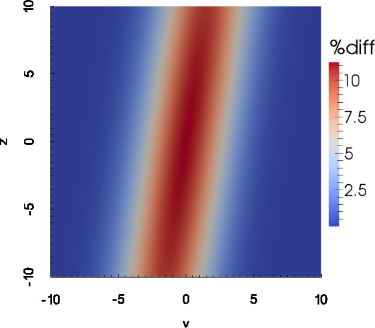
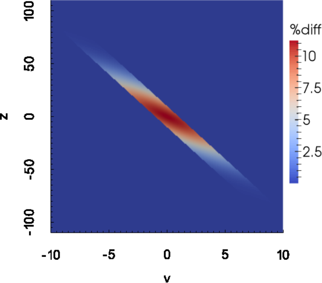
The use of %diff will show the distribution of error and thus show where the largest errors occur. For (1) and (4) the major contribution of errors is expected to be occur on the boundary, due to the interaction with the artificial boundary conditions. However, it is expected that for the self-similarity solution, Equation 5, the major contribution of error should be directly from discretization error rather than from imposed boundary conditions.

For purposes of comparing solutions and the contribution of errors from the FE discretization we first need exact solutions to each of the different forms of the Kolmogorov equation. To this end, we define the initial condition

f_{0}(v,x)=e^{-v^{2}-x^{2}}

(29)

and therefore the solution to (1), (4), and (5) are given by

$\displaystyle f_{\text{exact}}(t,v,x)$	$\displaystyle=\frac{\exp\left(-\frac{\left(3+3t^{2}+4t^{3}\right)v^{2}+6t(1+2t)vx+3(1+4t)x^{2}}{3+12t+4t^{3}+4t^{4}}\right)}{\sqrt{1+4t+\frac{4}{3}t^{2}+\frac{4}{3}t^{4}}},$	(30)
$\displaystyle g_{\text{exact}}(t,v,z)$	$\displaystyle=\frac{\exp\left(-\frac{(3+4t^{3})v^{2}+12t^{2}vz+3(1+4t)z^{2}}{3+12t+4t^{3}+4t^{4}}\right)}{\sqrt{1+4t+\frac{4}{3}t^{2}+\frac{4}{3}t^{4}}},$	(31)
$\displaystyle\widetilde{g}_{\text{exact}}(s,\widetilde{v},\widetilde{z})$	$\displaystyle=\frac{\exp\left(\frac{\left(1-4e^{s}\left(3+e^{s}\left(-3+e^{s}\right)\right)\right)v^{2}+12e^{s}\left(-1+e^{s}\right)^{2}vz-3e^{2s}\left(-3+4e^{s}\right)z^{2}}{-9+8e^{s}+12e^{2s}-12e^{3s}+4e^{4s}}\right)}{\sqrt{-3+\frac{8}{3}e^{s}+4e^{2s}-4e^{3s}+\frac{4}{3}e^{4s}}},$	(32)

respectively. Additionally, from Theorem 5 we see that the solution to (5) converges to

\widetilde{g}_{\infty}(\widetilde{v},\widetilde{z})=\frac{\sqrt{3}}{2}e^{-\widetilde{v}^{2}+3\widetilde{v}\,\widetilde{z}-3\widetilde{z}^{2}}

(33)

which is an elliptic Gaussian having magnitude $\frac{\sqrt{3}}{2}$ .

For the various forms of the Kolmogorov equations ((1), (4), (5)) we take the time interval, and problem domain to be respectively $I=[0,10],\quad\Omega=[-10,10]\times[-10,10]$ , which obviously satisfies Condition (13). For each equation we take the time step to be $\Delta t=\Delta s=0.01$ and the number of triangles along each side of the domain, $\Omega$ , to be $N=128$ .

Remark 5.1.

We note that while the starting domain for both (4) and (5) is given by $\Omega$ the respective change of variables results in the domain growing over time. Additionally, since $s$ is a scaling of the time, $t$ , we take the time interval for (5) to be $I_{s}=[0,2.4]$ which corresponds to $t\in I$ , since $t=e^{s}-1\Rightarrow s\in[0,\log(t-1)].$

For Equations (1) and (4) the support for the function grows beyond the problem domain in the given time interval, $I$ , and therefore the boundary conditions become more and more important as time increases until the solution, given by the FEM, no longer approximates the true solution of the original Cauchy problem. This can be seen in Figure 3 and Figure 4. Thus, as time increases the error becomes larger and larger, due to the diveregence from the exact solution caused by the interaction of the boundary conditions. While Equation (5) tends to a steady state with compact support in the domain $\Omega$ for the given time interval, therefore the approximation given by the FEM remains valid throughout the simulated time and should provide a better approximation to the exact solution for the Cauchy problem as can be seen in Figure 5. Additionally, we see in Table 1 that the $L^{2}$ -error at time $t=10$ is smaller for the self-similarity version of Kolmogorov, (5), as expected. In fact, the $L^{2}$ -error at $t=e^{10}-1$ is still smaller than the $L^{2}$ -errors associated with Equations (1) and (4) at $t=10$ and is

\|\widetilde{g}_{\text{exact}}(10,\widetilde{v},\widetilde{z})-\widetilde{g}(10,\widetilde{v},\widetilde{z})\|=0.0107995.

Algorithm 1	FEM applied to Equation 4	Algorithm 2
$0.0490644$	$0.0733016$	$0.019473$

Table 1:

L^{2}

-error for the FE discretizations at

t=10

While we have no theory predicting the exact convergence of the FEM applied to (5) we present observed convergence rates, so as to demonstrate that our solution is indeed a good approximation to the true solution. To this extent we see in Table 2 that the rate of convergence appears to follow the classical quadratic convergence rate expected for linear finite elements and the convergence rate is given by the least squares fit

E(h)=0.49796\,h^{2.0401}.

This convergence rate can also be observed in 2a.

$h$	$L^{2}$ -error	order
$1.00000$	$6.27854\times 10^{-1}$	$-$
$0.50000$	$9.90501\times 10^{-2}$	$2.6642$
$0.25000$	$2.70934\times 10^{-2}$	$1.8702$
$0.12500$	$6.94450\times 10^{-3}$	$1.9640$
$0.06250$	$1.74641\times 10^{-3}$	$1.9915$
$0.03125$	$4.36256\times 10^{-4}$	$2.0011$
$0.01562$	$1.08071\times 10^{-4}$	$2.0132$

Table 2:

L^{2}

-errors for FEM applied to the self-similar Kolmogorov equation, (5), at

s=10

with

dt=0.01

In addition to the phenomenon of decreasing $L^{2}$ -error for the FE approximation to (5) we would like to bring attention back to the phenomenon mentioned in Proposition 4 relating to the $L^{\infty}$ -norm of (5) not being monotonic. Indeed, the numerical simulation of (5) by FEM follows the same behavior as predicted by Proposition 4 and can be seen in 2b. In this simulation we observe that the initial solution behavior was for the $L^{\infty}$ -norm to increase and then eventually decrease to a steady state as expected.

(a) Observed rate of convergence in

L^{2}

-norm. The least squares fit is given by

E(h)=0.49796\,h^{2.0401}

(b) Observed

L^{\infty}

-norm and

L^{2}

-norm over time,

s

Fig. 2: Rate of convergence, 2a, and the observed

L^{\infty}

-norm and

L^{2}

-norm over time, 2b, for FEM and Algorithm 2 applied to (5)

Refer to caption — (a) Simulated solution

Remark 5.2.

We note that the change of variable $z=x+t\,v$ results in the rotation of the initial condition in the opposite direction to the direction seen in the original variables. This is apparent in the both the exact solution given in (6) and the simulations presented in Section 5, especially in Figure 4 and in Figure 5.

6 Conclusions

In this paper we introduce a discretization of the self-similar equation (5) based on an operator splitting technique combined with a finite element method and provide theoretical results for the method. Then in Section 5 we verified our theoretical results. The effectiveness of the self-similar change of variables was demonstrated in Section 5, by comparing finite element solutions for (1) using the method of splitting in Algorithm 1, the change of variables form of Kolmogorov (4), and the self-similar version of Kolmogorov (5). The self-similar change of variables had the lowest $L^{2}$ -error as compared to the solutions for (1) and (4). The main reason for this was due to the interaction of the artificially imposed boundary conditions with the solution on the inside of the domain. This is exactly as expected. We note that the self-similar change of variables solution can also suffer from the same draw back of artificial boundary conditions if a domain which is too small is chosen. However, the key point here is that the domain required is much smaller than that of (1) and (4), allowing for efficient long time simulation. In addition to the ability to use much smaller domains for long time simulation, the self-similar change of variables allows for fast marching in time due to the change in time from $t$ to $s$ where $t=e^{s}-1$ . Thus, time marching is exponential which adds to the efficiency of computing solutions to the self-similar change of variables version of the Kolmogorov equation. In summary we see that for long time integration the self-similar change of variables has the following benefits, as compared to the original formulation of the Kolmogorov equation: small space domain, and fast marching in time.

Acknowledgements

The authors would like to thank Professor Enrique Zuazua for suggesting this research topic and his great guidance while supervising this work. This work is supported by the Advanced Grants NUMERIWAVES/FP7-246775 of the European Research Council Executive Agency, FA9550-14-1-0214 of the EOARD-AFOSR, PI2010-04 and the BERC 2014-2017 program of the Basque Government, the MTM2011-29306-C02-00, and SEV-2013-0323 Grants of the MINECO.

During this research, the second author was member of the Basque Center for Applied Mathematics and he thanks the BCAM for its hospitality and support.

References

[1] K. Beauchard and E. Zuazua. Some controllability results for the 2D Kolmogorov equation. Ann. Inst. H. Poincaré Anal. Non Linéaire, 26(5):1793–1815, 2009.
[2] M. Berger and R. V. Kohn. A rescaling algorithm for the numerical calculation of blowing-up solutions. Comm. Pure Appl. Math., 41(6):841–863, 1988.
[3] M. Bessemoulin-Chatard. A finite volume scheme for convection-diffusion equations with nonlinear diffusion derived from the Scharfetter-Gummel scheme. Numer. Math., 121(4):637–670, 2012.
[4] M. Bessemoulin-Chatard and F. Filbet. A finite volume scheme for nonlinear degenerate parabolic equations. SIAM J. Sci. Comput., 34(5):B559–B583, 2012.
[5] C. J. Budd, G. J. Collins, and V. A. Galaktionov. An asymptotic and numerical description of self-similar blow-up in quasilinear parabolic equations. J. Comput. Appl. Math., 97(1-2):51–80, 1998.
[6] C. Buet and K.-C. Le Thanh. About positive, energy conservative and equilibrium state preserving schemes for the isotropic fokker-planck-landau equation. Preprint.
[7] O. Calin, D.-C. Chang, and H. Fan. The heat kernel for Kolmogorov type operators and its applications. J. Fourier Anal. Appl., 15(6):816–838, 2009.
[8] C. Chainais-Hillairet and F. Filbet. Asymptotic behaviour of a finite-volume scheme for the transient drift-diffusion model. IMA J. Numer. Anal., 27(4):689–716, 2007.
[9] J. Chang and G. Cooper. A practical difference scheme for fokker-planck equations. Journal of Computational Physics, 6(1):1–16, 1970.
[10] M. Escobedo and E. Zuazua. Self-similar solutions for a convection-diffusion equation with absorption in ${\bf R}^{N}$ . Israel J. Math., 74(1):47–64, 1991.
[11] M. Escobedo and E. Zuazua. Long-time behavior for a convection-diffusion equation in higher dimensions. SIAM J. Math. Anal., 28(3):570–594, 1997.
[12] A. Fiebach, A. Glitzky, and A. Linke. Uniform global bounds for solutions of an implicit Voronoi finite volume method for reaction–diffusion problems. Numer. Math., 128(1):31–72, 2014.
[13] F. Filbet and T. Rey. A rescaling velocity method for dissipative kinetic equations. applications to granular media. Journal of Computational Physics, 248(0):177 – 199, 2013.
[14] F. Filbet and G. Russo. A rescaling velocity method for kinetic equations: the homogeneous case. Proceedings Modelling and Numerics of Kinetic Dissipative Systems, Lipari, Italy, 2004.
[15] L. Gerardo-Giorda and M. B. Tran. Parallelizing the kolmogorov-fokker-planck equation. ESAIM: Mathematical Modelling and Numerical Analysis, eFirst, 10 2014.
[16] A. Glitzky. Uniform exponential decay of the free energy for Voronoi finite volume discretized reaction-diffusion systems. Math. Nachr., 284(17-18):2159–2174, 2011.
[17] L. Hörmander. Hypoelliptic second order differential equations. Acta Math., 119:147–171, 1967.
[18] W. Huang, J. Ma, and R. D. Russell. A study of moving mesh PDE methods for numerical simulation of blowup in reaction diffusion equations. J. Comput. Phys., 227(13):6532–6552, 2008.
[19] K. Igari. Degenerate parabolic differential equations. Publ. Res. Inst. Math. Sci., 9:493–504, 1973/74.
[20] A. Kolmogoroff. Zufällige Bewegungen (zur Theorie der Brownschen Bewegung). Ann. of Math. (2), 35(1):116–117, 1934.
[21] R. J. LeVeque. Finite Difference Methods for Ordinary and Partial Differential Equations: Steady-State and Time-Dependent Problems. Classics in Applied Mathematics Classics in Applied Mathematics. Society for Industrial and Applied Mathematics, Philadelphia, PA, USA, 2007.
[22] N. R. Nassif, N. Makhoul-Karam, and Y. Soukiassian. Computation of blowing-up solutions for second-order differential equations using re-scaling techniques. J. Comput. Appl. Math., 227(1):185–195, 2009.
[23] R. Plato. Large time asymptotics for a fully discretized fokker-planck type equation. Preprint.
[24] F. Rossi. Large time behavior for the heat equation on Carnot groups. NoDEA Nonlinear Differential Equations Appl., 20(3):1393–1407, 2013.
[25] R. D. Russell, J. F. Williams, and X. Xu. MOVCOL4: a moving mesh code for fourth-order time-dependent partial differential equations. SIAM J. Sci. Comput., 29(1):197–220 (electronic), 2007.
[26] V. Thomée. Galerkin finite element methods for parabolic problems, volume 25 of Springer Series in Computational Mathematics. Springer-Verlag, Berlin, 1997.
[27] C. Villani. Hypocoercive diffusion operators. In International Congress of Mathematicians. Vol. III, pages 473–498. Eur. Math. Soc., Zürich, 2006.

		$\displaystyle\int_{a}^{b}\int_{\alpha(w)}^{\beta(w)}\!\|g(w+s,ts)\|^{2}\,ds\,dw$
		$\displaystyle\hskip 28.45274pt=\int_{a}^{b}\int_{0}^{\beta(w)-\alpha(w)}\!\|g(w+\alpha(w)+s,ts+t\alpha(w))\|^{2}\,ds\,dw$
		$\displaystyle\hskip 28.45274pt\leqslant\int_{a}^{b}\int_{0}^{\beta(w)-\alpha(w)}s\int_{0}^{s}\!\|\partial_{w}g(w+\alpha(w)+\sigma,t\sigma+t\alpha(w))+t\partial_{z}g(w+\alpha(w)+\sigma,t\sigma+t\alpha(w))\|^{2}\,d\sigma\,ds\,dw$
		$\displaystyle\hskip 28.45274pt\leqslant\int_{a}^{b}\int_{0}^{\beta(w)-\alpha(w)}s\int_{\alpha(w)}^{\beta(w)}\,\|\partial_{w}g(w+\sigma,t\sigma)+t\partial_{z}g(w+\sigma,t\sigma)\|^{2}\,d\sigma\,ds\,dw$
		$\displaystyle\hskip 28.45274pt\leqslant\int_{a}^{b}\frac{(\beta(w)-\alpha(w))^{2}}{2}\int_{\alpha(w)}^{\beta(w)}\,\|\partial_{w}g(w+\sigma,t\sigma)+t\partial_{z}g(w+\sigma,t\sigma)\|^{2}\,d\sigma\,dw$
		$\displaystyle\hskip 28.45274pt\leqslant\frac{1}{2}\sup_{w\in[a,b]}\left((\beta(w)-\alpha(w))^{2}\right)\int_{a}^{b}\int_{\alpha(w)}^{\beta(w)}\!\|\partial_{w}g(w+\sigma,t\sigma)+t\partial_{z}g(w+\sigma,t\sigma)\|^{2}\,d\sigma\,ds\,dw.$

A Structure Preserving Scheme for the Kolmogorov-Fokker-Planck Equation

Abstract

keywords

AMS

1 Introduction

Remark 1.1.

2 Kernel and Long Time Behavior

2.1 Kernel

Proposition 1.

2.2 Long Time Behavior of the Kolmogorov Equation

Lemma 2.

Proof.

Corollary 3.

Proof.

3 Self-similar formulation of the Kolmogorov operator

Proposition 4.

Remark 3.1.

Proof.

Theorem 5 (The long time behavior of g~\widetilde{g}).

Proof.

4 Discretization Schemes

4.1 Restriction to a bounded domain

4.1.1 The Original Form

4.1.2 The Lagrangian Form

Lemma 6.

Proof.

4.1.3 The Self-Similar Form

Proposition 7.

Proof.

4.2 Weak forms and finite element discretization

Lemma 8.

4.3 Operator Splitting Methods

4.3.1 Operator Splitting for Kolmogorov Equation

4.3.2 An Exact Splitting Scheme

Theorem 9.

Proof.

Corollary 10.

Proof.

5 Numerical Results

Remark 5.1.

Remark 5.2.

6 Conclusions

Acknowledgements

References

Theorem 5 (The long time behavior of $\widetilde{g}$ ).