Probing the collective excitations of a spinor polariton fluid

For a general wave-vector ${\mathbf{k}}$ (as for ${\mathbf{k}}_{pb}$, here ${\mathbf{k}}$ is assumed to be measured with respect to the pump wave-vector ${\mathbf{k}}_{p}$), the different branches of the spectrum of excitations are the eigenvalues of the Bogoliubov operator $\hat{\mathcal{L}_{{\mathbf{k}}}}$ and thus are evaluated starting from the equation:

or equivalently finding the roots of the following polynomial equation:

This can be solved exactly, resulting in four branches of the spectrum, which, as explained later, we label with a new index $a=u_{\uparrow},v_{\uparrow},u_{\downarrow},v_{\downarrow}$:

where $\eta_{u,v}=\pm 1$ for the particle-like and hole-like components respectively and $\sigma_{\uparrow,\downarrow}=\pm 1$. Here, the energy

determines the excitation spectrum of two independent fluids with opposite circular polarisations, which is given by [5, 27]

When setting $\psi_{-}=0$ (circular polarization) or $\psi_{+}=\psi_{-}$ (linear polarization), one recovers the limiting expressions derived in Ref. [18].

Note that, because of interactions, polarisation and particle-hole degrees of freedom do in general mix together along the dispersion of each spectrum branch. Yet, the choice of the index $a=u_{\uparrow},v_{\uparrow},u_{\downarrow},v_{\downarrow}$ for labeling the four branches of the excitation spectrum is motivated by the fact that, at large momenta there is no mixing between the particle-like ($u_{\uparrow,\downarrow}$) and hole-like ($v_{\uparrow,\downarrow}$) degrees of freedom, while the same does not hold of $+$ and $-$ polarisation states that do remain coupled — i.e., as we will see later, the intrinsic polarisation of these branches can never be purely circularly $+$ or $-$ polarised even at large momenta, where the energy becomes

where $\psi_{\uparrow,\downarrow}\equiv\psi_{+,-}$. For this reason, we introduces a new notation $\uparrow,\downarrow$ for the branch index $a=(u_{\uparrow},v_{\uparrow},u_{\downarrow},v_{\downarrow})$, indicating that the pure circular polarisation degrees of freedom $\pm$ are always coupled.

We now classify all possible different types of excitation spectra (see Fig. 4) and how these evolve from one type to the other by changing the system parameters, as represented in the “phase diagram” of Fig. 3. Interestingly, for a fixed interaction strength ratio $\alpha_{2}/\alpha_{1}$ ($=-0.1$ in the figures), only two dimensionless independent parameters are sufficient in order to classify all possible different types of spectra of a resonantly pumped spinor polariton fluid: 1) the mean-field polarisation angle $\theta_{0}$ (4) and 2) the dimensionless pump energy rescaled by the “self-interaction” energy $\mathcal{E}=\alpha_{1}(|\psi_{+}|^{2}+|\psi_{-}|^{2})$:

By means of these two parameters only we can fully classify all the allowed spectrum typologies. Note in fact that the value of the pump momentum ${\mathbf{k}}_{p}$ has the sole effect of tilting the spectrum dispersion; in the quadratic approximation for the LP dispersion considered here, this corresponds to a Galilean transformation. [28] For this reason, we plot, without loss of generality, the spectra of Fig. 4 for a pump in the orthogonal direction to the cavity growth, ${\mathbf{k}}_{p}=0$.

In the absence of inter-polarisation interaction, $\alpha_{2}=0$, and for equal spin populations, $|\psi_{+}|=|\psi_{-}|$, both sign and value of a single parameter, the rescaled interaction renormalised pump detuning $\bar{\Delta}=\Delta/\alpha_{1}|\psi_{+}|^{2}$, determine the four types of possible spectra [5, 27]: 1) for $\Delta<0$ the spectrum is gapped; 2) the gap closes to zero for $\Delta=0$ and the dispersion is linear at low momenta; while for $\Delta>0$, particle and hole branches of the spectrum real part touch together in either 3) one ($\bar{\Delta}\leq 2$) or 4) two ($\bar{\Delta}>2$) separate momentum intervals — note that Fig. 4 is a cut at $k_{y}=0$, so intervals for those plots in reality corresponds to rings in the two-dimensional ${\mathbf{k}}$-space. Both cases 3) and 4) are generally named as diffusive spectra. Note that the linear spectrum is allowed for a single value of the detuning $\Delta$, and thus even if the types of different spectra for $\alpha_{2}=0$ are four in total, the finite interval regions in $\Delta$ displaying different spectra are only three (and $\Delta=0$ represents a separating point between two of these regions). For the spinor case, the minimal set of independent dimensionless parameters characterising the spectrum is instead formed by $\theta_{0}$ and $\bar{\omega}_{p}$. Note that by rescaling the pump detuning $\Delta_{\pm}$ (14) by the self-interaction energy $\mathcal{E}$ would still lead to a parameter depending on $\theta_{0}$.

For a coupled spinor fluid, with $\alpha_{2}\neq 0$, the classes of different spectra increase from four to eighteen; by counting the parameter finite regions only (and excluding the separating lines), this corresponds to nine regions of different spectra compared to the three of the previous $\alpha_{2}\to 0$ limit case. The proliferation of different types of spectra is due to the presence of two nested square roots in Eq. (16). Which of the four branches have a degenerate real part as well as in how may momentum intervals degeneracy occurs, depends on the sign of both square root arguments. All nine possibilities for the spectra are plotted in Fig. 4 and the various “phase diagram” regions in the $(\bar{\omega}_{p},\theta_{0})$ parameter space where such spectra are allowed are plotted in Fig. 3.

For both negative as well as small positive values of the renormalised dimensionless pump energy detuning, $\bar{\omega}_{p}$, the spectrum is fully gapped, i.e., none of the four branches mix together (panel $1$ in Fig. 4). By increasing the value of $\bar{\omega}_{p}$ at fixed $\theta_{0}$, the $\uparrow$ branches (black lines) are still gapped, while the real part of the particle-like $u_{\downarrow}$ (thick red-gray) and hole-like $v_{\downarrow}$ (thin red-gray) branches undergo the same changes as previously described for a single component fluid: they touch each other first in a single momentum interval (panel $2$) and then in two separate momentum intervals (panel $3$).

Even if for panels $2$ and $3$ the $\downarrow$ branches have a diffusive-like character, with an imaginary part deviating from the polariton lifetime, $\Im\omega\neq-\gamma/2$, in all the three regimes $1-3$ described, the $\uparrow$ and $\downarrow$ real part branches are never degenerate and hence do not mix one with the other, so that each maintains its own character: we group the three cases as gapped spectra (white region of Fig. 3).

When we further increase the value of $\bar{\omega}_{p}$, the opposite polarisation branches can however mix together and the spectrum evolves differently depending on the value of the mean-field polar angle $\theta_{0}$: in particular it either changes from the type $3$ to $7$ if $\theta_{0}<\theta_{0}^{\text{cr}}$, or from $2$ to $4$ if $\theta_{0}>\theta_{0}^{\text{cr}}$, where the critical angle $\theta_{0}^{\text{cr}}$ is given by:

For $\alpha_{2}/\alpha_{1}=-0.1$, this critical value of the polarisation angle is given by $\theta_{0}^{\text{cr}}\simeq 0.54$. The dash-dotted line in Fig. 3 indicates where $\theta_{0}^{\text{cr}}$ determines the boundary between these two cases. The difference between the two is how the $\uparrow$ and $\downarrow$ branches mix together and at which energy the mixing happens. For $\theta_{0}>\theta_{0}^{\text{cr}}$, there is only mixing of the branches at zero energy, as for the three spectra $4-6$, which we group under the naming $0$-diffusive (clear gray region of Fig. 3). When $\theta_{0}<\theta_{0}^{\text{cr}}$, the spectra are characterized by the presence of a diffusive momentum region at finite energy, as for the spectra $7-9$, that we group under the naming $\omega$-diffusive spectra (dark gray region of Fig. 3).

If we increase $\bar{\omega}_{p}$ for $\theta_{0}>\theta_{0}^{\text{cr}}$, the branches transforms via different $0$-diffusive phases. For the spectrum of type $4$ all four branches real parts are degenerate at $\omega=0$ around ${\mathbf{k}}=0$, this then evolves to a zero energy degeneracy in different parts of the momentum space for the cases $5$ and $6$. When $\bar{\omega}_{p}$ is instead increased for $\theta_{0}<\theta_{0}^{\text{cr}}$, the $\uparrow$ branch transforms via different $\omega$-diffusive phases: Here, we get a mixing of the $u_{\uparrow}$ ($v_{\uparrow}$) branch with the $u_{\downarrow}$ ($v_{\downarrow}$) branch as in the panel $7$, where there is a narrow region in ${\mathbf{k}}$ space where the spectrum is diffusive and $\Re\omega\neq 0$. Note that for these spectral types the four branches cannot be degenerate all at the same time as in the $0$-diffusive case previously considered; now only two branches at the time get degenerate, while the other two do repel each other. Higher values of $\bar{\omega}_{p}$ induce a similar behaviour but for different intervals of momentum, as for region $8$ or region $9$. Degeneracy at zero energy is however still possible for the $\downarrow$ branch, as seen in panels $8$ and $9$.

The spectral phases of a circularly (linearly) polarized fluid are the ones found on the line $\theta_{0}=0$ ($\theta_{0}=\pi/4$) and coincide with the results discussed in Ref. [18]. After having classified completely all possible excitation spectra, we now discuss in the next section their intrinsic polarisation properties.

Each mode of the collective spectrum does emit with an intrinsic degree of polarisation along the dispersion. This can be determined by starting from the eigenvalue equations,

where $\omega_{\mathbf{k}}^{(a)}$ are the four branches (16) labeled by the index $a=u_{\uparrow},v_{\uparrow},u_{\downarrow},v_{\downarrow}$ and ${\mathbf{x}}^{(a)}_{\mathbf{k}}$ are the four four-component eigenvectors of the Bogoliubov matrix $\hat{\mathcal{L}}_{{\mathbf{k}}}$, ${\mathbf{x}}^{(a)}_{{\mathbf{k}}}=(x_{u_{+},{\mathbf{k}}}^{(a)},x_{v_{+},{\mathbf{k}}}^{(a)},x_{u_{-},{\mathbf{k}}}^{(a)},x_{v_{-},{\mathbf{k}}}^{(a)})$ — thus here the lower indices $u_{+},v_{+},u_{-},v_{-}$ specify the eigenvector component, while the upper indices $(a)$ refer to the eigenvalue branch.

For each branch labeled by $(a)$ and for a given direction ${\mathbf{k}}$ (measured with respect to the pump wave-vector ${\mathbf{k}}_{p}$) we might expect that, out of a $4$-component complex vector ${\mathbf{x}}^{(a)}_{{\mathbf{k}}}$, the degree of polarisation will be characterised by two polar angles and by two azimuthal angles, all independent from each other. However, the particle-hole symmetry which characterises the Bogoliubov matrix (9) leads to a redundancy of parameters. In particular, the Bogoliubov matrix (9) is symmetric under the simultaneous exchange of the $u\leftrightarrow v$ components and the transformation $\hat{\mathcal{L}}_{{\mathbf{k}}}=-\hat{{\mathcal{L}}}_{-{\mathbf{k}}}^{*}$. For eigenvalues and eigenvectors this implies that

where $j=\uparrow,\downarrow$. Thus, in order to characterise the intrinsic degree of polarisation of the collective spectrum, it is enough to define a “normal” polar polarisation angles for each of the two $j=\uparrow,\downarrow$ particle-like branches as

In fact, for the hole-like branches, we have that $\cos(2\theta_{j,{\mathbf{k}}})=|x_{v_{+},-{\mathbf{k}}}^{(v_{j})}|^{2}-|x_{v_{-},-{\mathbf{k}}}^{(v_{j})}|^{2}$ — we are assuming here the following normalisation conditions for the eigenvector components, $|x_{u_{+},{\mathbf{k}}}^{(u_{j})}|^{2}+|x_{u_{-},{\mathbf{k}}}^{(u_{j})}|^{2}=1=|x_{v_{+},-{\mathbf{k}}}^{(v_{j})}|^{2}+|x_{v_{-},-{\mathbf{k}}}^{(v_{j})}|^{2}$. Similarly, we can also define two “anti-normal” polar polarisation angles as:

where $I_{j,{\mathbf{k}}}=|x_{u_{+},{\mathbf{k}}}^{(v_{j})}|^{2}+|x_{u_{-},{\mathbf{k}}}^{(v_{j})}|^{2}=|x_{v_{+},-{\mathbf{k}}}^{(u_{j})}|^{2}+|x_{v_{-},-{\mathbf{k}}}^{(u_{j})}|^{2}$ is the normalisation of the anti-normal modes with respect to the normalisation of the normal ones which was fixed to $1$. Thanks to the particle-hole symmetry, we could have equivalently defined these angles as $I_{j}\cos(2\eta_{j,{\mathbf{k}}})=|x_{v_{+},-{\mathbf{k}}}^{(u_{j})}|^{2}-|x_{v_{-},-{\mathbf{k}}}^{(u_{j})}|^{2}$. To summarise, for each branch we have two polar angles $\theta$ and $\eta$ determining the degree of polarisation of the collective emission. These are not directly measurable quantities. However, in the pump-probe experiment proposed and analysed in the next section, the normal angle $\theta$ is related to the resonant transmission of the particle modes along the particle-like probe direction ${\mathbf{k}}_{p}+{\mathbf{k}}_{pb}$, while the anti-normal angle $\eta$ to the transmission along the hole-like direction ${\mathbf{k}}_{p}-{\mathbf{k}}_{pb}$.

We now analyse in the bottom panels of Fig. 5, the behaviour of both $\theta_{j,{\mathbf{k}}}$ (thick lines) and $\eta_{j,{\mathbf{k}}}$ (thin lines) along each branch dispersion for three representative spectra (top panels) of the gapped, $0$-diffusive, and $\omega$-diffusive types previously classified in Figs. 3 and 4. Let us first note that it can be easily shown that the intensity $I_{j,{\mathbf{k}}}$ decays quickly to zero at large momenta, i.e. $I_{j,{\mathbf{k}}}\sim k^{-4}$ for $k\gg\sqrt{m\mathcal{E}}$, where $\mathcal{E}=\alpha_{1}(|\psi_{+}|^{2}+|\psi_{-}|^{2})$. This implies that, in this limit, the coupling between particle-like and hole-like degrees of freedom can be neglected, allowing us to find the asymptotic behaviour of the normal polarisation angles at large momenta:

where $\sigma_{j=\uparrow,\downarrow}=\pm 1$ and $\tan(2\theta_{0})=2|\psi_{+}||\psi_{-}|/(|\psi_{+}|^{2}-|\psi_{-}|^{2})$.

As panel (d) of Fig. 5 shows, for a gapped spectrum (panel (a), corresponding to spectrum 1 in Fig. 4) the angles $\theta_{\uparrow,{\mathbf{k}}}$ (thick black line) and $\theta_{\downarrow,{\mathbf{k}}}$ (thick red-gray line) vary only very little along the dispersion because there is no mixing between $\uparrow$ and $\downarrow$ branches. In particular, while for the $\uparrow$ branch the normal degree of polarisation (thick black) is almost everywhere fully left-polarised, $\theta_{\uparrow,{\mathbf{k}}}\simeq 0$ (corresponding to the north pole of the Poincaré sphere in Fig. 1), for the $\downarrow$ branch (thick red-gray line) $\theta_{\downarrow,{\mathbf{k}}}\simeq\pi/2$ (south pole). Both anti-normal angles $\eta_{j,{\mathbf{k}}}$ (thin lines) also display a small variation along the dispersion from the values $\eta_{\uparrow,{\mathbf{k}}}\simeq 0$ (thin black) and $\eta_{\downarrow,{\mathbf{k}}}\simeq\pi/2$ (thin red-gray).

Mixing of the $\uparrow$ and $\downarrow$ branches causes instead sudden changes of both normal and antinormal angles along each dispersion. This is the case of both the $0$-diffusive spectrum shown in panel (b) of Fig. 5 (corresponding to panel 5 of Fig. 4) as well as the $\omega$-diffusive spectrum shown in panel (c) (and corresponding to the spectrum 7 of Fig. 4), even if the mixing happens in different ways. In particular, for the $0$-diffusive spectrum, different branches touch each other in two separated regions in ${\mathbf{k}}$-space. The branches $u_{\downarrow}$ and $v_{\downarrow}$ mix together for $k\lesssim 1.5\sqrt{m\mathcal{E}}$, where the angles $\theta_{\downarrow,{\mathbf{k}}}$ and $\eta_{\downarrow,{\mathbf{k}}}$ coincide. Inside this region, there is a another region where also the $u_{\uparrow}$ and $v_{\uparrow}$ mix together. Here, also the angles $\theta_{\uparrow,{\mathbf{k}}}$ and $\eta_{\uparrow,{\mathbf{k}}}$ will coincide. In between these mixing regions, the values of the angles undergo a sudden change in value from almost a purely left-circularly polarised degree to a right-circularly polarised degree.

The last case we analyse is the $\omega$-diffusive spectrum shown in panel (c) of Fig. 5. The difference with the case previously considered of a $0$-diffusive spectrum, lies in the fact that now all four real part branches do not become degenerate in the same momentum region and that the degeneracy of $\uparrow$ and $\downarrow$ branches is allowed at finite energy. Aside these differences in how $\uparrow$ and $\downarrow$ branches do mix with each other, we observe in panel (f) a similar sudden flip of both normal and anti-normal polar angles along the dispersion that we also observed for the $0$-diffusive spectrum in panel (e).

After having discussed the intrinsic properties of the collective spectrum, including the emission degree of polarisation along the dispersion of each branch, we derive now the response of the spinor fluid to an additional probe beam and how this is related to the intrinsic spectral properties discussed so far. To this end, we go back to the system linear response (8) to a weak external probe shined at a direction ${\mathbf{k}}_{p}+{\mathbf{k}}_{pb}$ and an energy $\omega_{p}+\omega_{pb}$. Eq. (8) can be easily inverted to give the system response ${\mathbf{w}}=(u_{+},v_{+},u_{-},v_{-})^{T}$ in terms of the probe vector ${\mathbf{f}}^{pb}=(f_{+}^{pb},0,f_{-}^{pb},0)^{T}$:

As explained previously, and also illustrated in the schematic set-up of Fig. 2, the intensity of the response in the direction ${\mathbf{k}}_{p}+{\mathbf{k}}_{pb}$ will be given by the particle-like component $|u_{\pm}|^{2}$, while the one at the direction ${\mathbf{k}}_{p}-{\mathbf{k}}_{pb}$, by the hole-like component $|v_{\pm}|^{2}$ — from now onwards, we will consider the particular case of a pump shined orthogonally to the cavity plane, ${\mathbf{k}}_{p}=0$. From Eq. (26), we expect that the response will be enhanced when $(\omega_{pb},{\mathbf{k}}_{pb})$ is scanned close to one of the branches of the collective excitation spectrum, i.e., the eigenvalues of the Bogoliubov matrix $\hat{\mathcal{L}}_{{\mathbf{k}}_{pb}}$. Because the spectrum is complex, we expect a broadened enhanced emission — typically of the order of the polariton linewidth $\gamma$, with variations in the diffusive regions in momentum space where different branches touch each other and the imaginary part of the spectrum deviates from the polariton lifetime $\gamma$. While the resolution in energy is limited by the imaginary part of the spectrum, the resolution in momentum space can only suffer experimental limitations, such as the angular resolution of the detection device and the intrinsic angular width of the probe beam. The probe beam resolution in momentum can be improved by considering a large enough homogeneous profile [29].

We express the probe vector ${\mathbf{f}}^{pb}$ in terms of the polar $\theta_{pb}$ and azimuthal $\phi_{pb}$ angles, quantifying the polarisation degree of the probe:

where $|f^{pb}|^{2}$ is the probe beam intensity. We set $\phi_{pb}=0$. Similarly, the response ${\mathbf{w}}$ can be conveniently parametrised in terms of the particle-like $I_{u}=|u_{+}|^{2}+|u_{-}|^{2}$ and hole-like $I_{v}=|v_{+}|^{2}+|v_{-}|^{2}$ intensities, as well as the polar angles $\theta_{u,v}$ along the two directions $\pm{\mathbf{k}}_{pb}$:

Finally, as already discussed, we assume that the pump induces a mean-field state with $\phi_{0}=0$ and $\theta_{0}\in[0,\pi/4]$ (4).

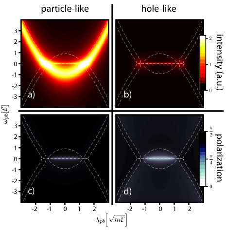
We plot in Figs. 6 and 7 the two-dimensional maps for both intensities $I_{u,v}$ and polar angles $\theta_{u,v}$ for the response to a probe beam by scanning different values of the the probe energy $\omega_{pb}$ and momentum ${\mathbf{k}}_{pb}$. We choose the particular case of a gapped spectrum (Fig. 6), corresponding to the same conditions as panels (a) and (d) of Fig. 5 and the case of a $0$-diffusive spectrum (Fig. 7), corresponding to the same conditions as panels (b) and (e) of Fig. 5. We first note that, as expected, the probe beam (27) has only a finite strength in the particle-like channels and cannot directly excite hole-like quasi-particles. Nevertheless, the response has a finite emission intensity also for the hole-like branches because of the interactions mixing together particle and hole degrees of freedom. As previously illustrated in Eq. (19) particle and hole modes asymptotically decouple one from the other at large momenta. We thus expect that the response emission intensity quickly drops to zero for all hole-like branches. In panel (b) of Fig. 6 this behaviour is clearly visible, as the emission intensity of the hole branches is strongly reduced with respect to the one of the particle branches.

In the previous section we have seen that each branch of the collective excitation spectrum is characterised by an intrinsic degrees of polarization, quantified by the normal ($\theta_{\uparrow,\downarrow}$) and anti-normal ($\eta_{\uparrow,\downarrow}$) polar angles. In Fig. 6, the gapped spectrum is probed with a linearly polarized beam, $\theta_{pb}=\pi/4$. Here, we obtained an enhanced emission when the probe is in resonance with either the $u_{\uparrow}$ or the $u_{\downarrow}$ branch. We remind that for a gapped spectrum there is no mixing between the $\uparrow$ and $\downarrow$ degrees of freedom, and thus the $\theta_{\uparrow,\downarrow}$ angles only weakly deviate from their asymptotic values at large ${\mathbf{k}}$ (see Fig. 5), in this particular case almost purely circularly left or right polarized. Hence, one expects that the emission intensity for the $u_{\uparrow}$ and $u_{\downarrow}$ branches is comparable, since the linearly polarised probe couples identically to left- and right-polarized modes. In panel (c) of Fig. 6 we observe the polarization to undergo a rotation when in resonance with one of the spectral branches. As expected, probing at resonance with the $u_{\uparrow}$ branch results in a largely left-polarized emission, while the $u_{\downarrow}$ branch induces a right-circular polarization.

Interesting effects are observed for the case of diffusive spectra, and we show in particular the case of a $0$-diffusive spectrum in Fig. 7. For this case we consider the case of a right-circularly polarized probe beam ($\theta_{pb}=\pi/2$) so that we have a $u_{\downarrow}$ branch emitting much stronger than the $u_{\uparrow}$ branch (see panel (a) of Fig. 7). However, around ${\mathbf{k}}_{p}=0$, where the spectral branches mixed one the other in a diffusive region, we see that the resonant branch is not $u_{\downarrow}$, rather $v_{\uparrow}$. Here, the strongest emission intensity comes from the $u_{\downarrow}$ branch at large momenta and from the $v_{\uparrow}$ branch inside the diffusive region at small ${\mathbf{k}}$. Because of the mixing between $\uparrow$ and $\downarrow$ degrees of freedom, we have observed a sudden spin flip for the degree of polarisation of the eigenvectors around $|{\mathbf{k}}|\sim 1.2\sqrt{m\mathcal{E}}$. This is the reason for the resonant emission transfers from $u_{\downarrow}$ to $v_{\uparrow}$ at small ${\mathbf{k}}$. From panel (b) of Fig. 7 it is clear that, in the beam transferred in the $-{\mathbf{k}}_{pb}$ direction, the emission is the strongest in the diffusive momentum ring at $\omega_{p}=0$ where $u_{\downarrow}$ and $v_{\downarrow}$ are mixed. The stronger intensity for these modes can be explained in terms of an onset of parametric amplification. In fact, in this diffusive region the imaginary part of the spectrum part deviates from the value of the constant decay rate and there is an additional contribution from the negative argument of the outer root in Eq. (16) — see panel 5 in Fig. 4. For this reason, these modes acquire a longer lifetime, and therefore undergo enhanced scattering. Similarly, in panel (a) of Fig. 7, one can appreciate an increase in transmission in the same diffusive region. In addition, there is also an increased emission on the diffusive region at $\omega_{p}=0$ where the $u_{\downarrow}$ and $v_{\downarrow}$ branches are degenerate. Although, for these values of the momentum, these branches are circularly left polarized, the inter-spin interaction coupling the $\uparrow$ and $\downarrow$ modes, combined with the strong parametric amplification, still leads to a strong emission. It is interesting to note that in previous work [12], the proximity to an instability to a parametric scattering regime has been related to the occurrence of a negative drag force when a resonantly pumped polariton fluid scatters against a localised defect. Here, the same phenomenon leads to enhanced emission of parametrically amplified modes when the system is probed with an additional weak laser.

In panels (c) [(d)] of Fig 7 we plot the azimuthal polarization angle for particle-like (hole-like)transmitted signal at ${\mathbf{k}}_{pb}$ ($-{\mathbf{k}}_{pb}$). The resonant branch is $u_{\downarrow}$ at large ${\mathbf{k}}$ and $v_{\uparrow}$ for small values of the momentum and strongly emits circularly right polarized light — $\theta^{u}_{pb}\simeq\theta^{v}_{pb}\simeq\pi/2$. Yet the parametrically amplified region around ${\mathbf{k}}_{p}=0$ emits both in the transmitted ${\mathbf{k}}_{pb}$ and $-{\mathbf{k}}_{pb}$ directions an almost purely circularly left polarized light. Hence, the parametric amplification of the mixed $u_{\downarrow}$ and $v_{\downarrow}$ mode causes the left-polarized incoming probe light to undergo a spin flip when interacting with the polariton sample. We show in Fig. 8 that $\theta_{pb}^{u,v}$ tend to $0$ (i.e., almost pure left-polarization), when the parametric amplified mode ${\mathbf{k}}_{p}=0.5\sqrt{m\mathcal{E}}$, probed with $\omega_{pb}=0$, is brought closer to resonance by varying the polariton decay time $\gamma\to\gamma_{crit}^{-}$ — here $\gamma_{crit}$ is the minimum value of the polariton decay rate required for the system stability, i.e., $\Im\omega<0$. The emission intensity (panel (a) of Fig. 8) diverges as $1/(\gamma-\gamma_{crit})^{2}$ for both particle-like and hole-like signals when they are brought close to resonance. This can be understood from the expression (26), where we see that the right-hand side becomes singular if $\omega_{pb}$ equals $\Re\omega^{(a)}_{{\mathbf{k}}_{pb}}$ and at the same time $\Im\omega^{(a)}_{{\mathbf{k}}_{pb}}\to 0^{-}$. In this limit, the response ${\mathbf{w}}$ coincides with the eigenvector ${\mathbf{x}}^{(a)}$ of the Bogoliubov matrix $\hat{\mathcal{L}}_{{\mathbf{k}}_{pb}}$. Here, this is the case for ${\mathbf{x}}^{u_{-}}$, so that the polarization $\theta_{pb}$ of the response approaches $\theta_{\downarrow}|_{{\mathbf{k}}=0}=\eta_{\downarrow}|_{{\mathbf{k}}=0}\simeq 0.08$, as it can be seen in panel (b) of Fig. 8. Note that $\theta_{\downarrow}=\eta_{\downarrow}$ exactly in the diffusive disk around ${\mathbf{k}}=0$, where $u_{\downarrow}$ and $v_{\downarrow}$ coincide. In Fig. 8, we have measured the decay rate $\gamma$ in units of self-interaction energy $\mathcal{E}$.

Experimentally, however, $\gamma$ is fixed for a given microcavity, but the ratio $\gamma/\mathcal{E}$ can be tuned by varying the laser pump power, $|f^{p}|^{2}$ in Eq. (2). One should then calculate the mean-field equations (3) to derive the polariton spin densities $|\psi_{\pm}|^{2}$ and thus the self-interaction energy $\mathcal{E}$. By varying the tilting angle of the probe beam with respect to the pump, one can scan through ${\mathbf{k}}$-space. As depicted on Fig. 2, also the detectors should be placed accordingly: one at the same angle as the probe and the other at the mirrored angle, to detect the particle and the hole-like signal respectively. At each position of the probe, a vertical slice on the response figures can be reconstructed by changing the probe frequency $\omega_{pb}$ and measuring the intensity and polarization at both detectors.