Edge Corrections to Electromagnetic Casimir Energies From General-Purpose Mathieu Function Routines
Abstract
Scattering theory methods make it possible to calculate the Casimir energy of a perfectly conducting elliptic cylinder opposite a perfectly conducting plane in terms of Mathieu functions. In the limit of zero radius, the elliptic cylinder becomes a finite-width strip, which allows for the study of edge effects. However, existing packages for computing Mathieu functions are insufficient for this calculation, because none can compute Mathieu functions of both the first and second kind for complex arguments. To address this shortcoming, we have written a general purpose Mathieu function package, based on algorithms developed by Alhargan [1, 2]. We use these routines to find edge corrections to the proximity force approximation for the Casimir energy of a perfectly conducting strip opposite a perfectly conducting plane.
pacs
42.25.Fx, 03.70.+k, 12.20.-mI Introduction
Scattering theory methods have made it possible to calculate Casimir energies, arising from quantum-mechanical fluctuations of charges and fields in quantum electrodynamics, for any objects for which one can obtain the -matrices for light scattering. In this approach, one expresses the Casimir energy in “TGTG” form [3], generalizing scattering results for planar geometries [4] and for scalar fields in spherical geometries [5] to any geometry that is tractable for electromagnetic scattering [6, 7]. The resulting calculation combines the scattering -matrix, which captures the reflection of quantum fluctuations from each object individually, with the free Green’s function, which propagates fluctuations from one object to the other.
One geometry of particular interest is the electromagnetic cylinder, which in the limit of zero radius becomes a finite-width strip [8], allowing for the study of edge effects [8, 9, 10, 11, 12, 13, 14, 15]. These effects can be modeled as corrections to the proximity force approximation (for a situation where the derivative expansion [16, 17, 18] does not apply). However, numerical calculations of the Casimir energy in elliptic cylinder geometries require Mathieu functions [19, 20, 21, 22], in cases for which existing packages are not well-suited. As a result, we have created a general-purpose package to compute odd and even, angular and radial, first-kind and second-kind, and ordinary and modified Mathieu functions of integer order, for complex parameter and argument and integer index. Our approach is based on the routines developed by Alhargan [1, 2], extended to the case of complex inputs and implemented in Mathematica.
At short distances, we can expand the Casimir interaction energy per unit length of a perfectly conducting strip oriented parallel to a perfectly conducting plane as
| (1) |
where is the width of the strip, is the distance between the plane and the strip, and and are dimensionless constants. The leading term in this expansion gives the proximity force approximation; the second term gives the interaction of the two edges with the infinite plane; and the third term gives the interaction between the two edges, mediated by the plane. From an exact numerical calculation, we find good agreement with this form, with and . The former quantity agrees with results obtained at lower precision in Refs. [9, 10, 11, 23]; its small magnitude can be explained by the cancellation of the effects of the first reflection for electromagnetism [9, 24, 23].
In the following sections we assemble the various components needed to obtain this result. In Section II we review scattering theory in elliptic cylinder coordinates and establish conventions for the Mathieu functions that arise as solutions to the Helmholtz equation. Then in Section III we describe the numerical package we have developed to calculate these functions in the generality required for Casimir calculations. Finally, we discuss the results of the Casimir calculation in Section IV.
II Scattering Theory in Elliptic Cylinder coordinates
We begin by formulating scattering theory in elliptic cylinder coordinates,
| (2) |
where is the interfocal separation, is the analog of the angle in ordinary cylindrical coordinates, and is the analog of the ordinary cylindrical radius , with
| (3) |
The Helmholtz equation in elliptic cylinder coordinates is given by
| (4) |
Using separation of variables with gives
| (5) | |||||
| (6) | |||||
| (7) |
where the parameter is given by and the separation constant is known as the characteristic value. For we have the standard complex exponential solutions . Because the problem still has reflection symmetry, we have angular solutions that are either even or odd functions of the argument , the analogs of and in the ordinary cylinder case. We are interested only in characteristic values for which the resulting angular functions are periodic, which we label by the integer index , where runs from to for even solutions and from to for odd solutions. For and , the even and odd angular functions then reduce to and respectively, and the characteristic value becomes in both cases. For the special case of , in the limit as goes to zero the even angular function goes not to , but instead to the constant function , with characteristic value zero (and there is no odd angular function for ).
The radial solutions are the analogs of Bessel functions in ordinary cylindrical coordinates. We note that the radial functions obey the same differential equation as the angular functions with imaginary argument, a relationship we will make use of in our computational algorithm. Unlike the case of ordinary cylindrical functions, the radial functions corresponding to even and odd angular functions for the same index differ, because they have different characteristic values.
Because the Mathieu equations are second-order, they each have two independent solutions: solutions of the first kind obey appropriate regularity conditions at the origin, while solutions of the second kind do not. Furthermore, since , positive values of correspond to propagating waves, while negative values of correspond to evanescent waves; it will be convenient to define modified versions of all of our functions, which are related to the ordinary functions with . These choices — even and odd, angular and radial, ordinary and modified, and first-kind and second-kind — therefore yield a total 16 Mathieu functions. The four modified angular functions typically are not assigned their own names; the remaining 12 are summarized in Table 1.
| Angular | Radial | ||||||||||
| Ordinary | Ordinary | Modified | |||||||||
| First kind | Second kind | First kind | Second kind | First kind | Third kind | ||||||
| Even | Odd | Even | Odd | Even | Odd | Even | Odd | Even | Odd | Even | Odd |
We normalize our functions following the conventions of of Abramowitz and Stegun [20], but name them using a modified notation that is more closely analogous to the ordinary cylinder case. The even and odd angular functions and are normalized such that
| (8) |
which is analogous to the normalization of the ordinary trigonometric functions and (except for , as described above). The radial functions are all normalized so that they approach the analogous Bessel functions at large distances. These conventions are convenient for creating a standard expansion of free quantum fields in terms of Mathieu functions [25]. Also in analogy with Bessel functions, we define the modified functions by
| (9) |
and
| (10) |
for , where the radial functions of the third kind are given by and . As in the ordinary cylinder case, the definitions of and in terms of third kind functions yield the exponentially decaying evanescent solutions, avoiding the cancellation of large numbers that would be required to extract these solutions from the direct continuation to negative of the solutions first and second kind.
III Computation of Mathieu Functions
We have developed a package written in Mathematica for computing Mathieu functions. The built-in functionality of Mathematica supports only angular, first-kind functions (similar functionality is available in Maple). Since complex arguments are allowed, one can in principle obtain the radial first-kind functions as well. However, as described below, the standard calculation of angular functions is of limited utility for arguments with nonzero imaginary part; as a result, in that case we will need to use routines designed explicitly for the calculation of radial functions. We will also need second-kind functions to describe irregular scattering waves.
Our approach is based on methods developed by Alhargan [1, 2]. While these routines, written in C, support all 16 Mathieu functions and work reliably for all the inputs we have tested, they accept only positive and real arguments. We will therefore generalize these routines to complex argument and parameter, motivated by the Casimir calculation, which involves both angular functions of the first kind with complex argument and modified radial functions of the first and third kinds. Our code is available at http://community.middlebury.edu/˜ngraham .
III.1 Angular Functions for Real Argument
The standard calculation of angular Mathieu functions uses a Fourier series expansion,
| (11) | |||||
| with | (12) |
and
| (13) | |||||
| with | (14) |
Here the prefactors implement our normalization convention for the angular functions (which differs from that used by Alhargan). To obtain the coefficients and , we follow Alhargan and use both upward and downward recurrence relations for the ratios of adjacent coefficients. These recurrences start from zero and infinity respectively, and then meet at . The forms are slightly different for the even and odd functions and for odd and even order .
For the even function coefficients, denoting the even characteristic values as we have the following recursions,
| Even order | Odd order | (15) | |||
| (16) |
for with the base cases
| (17) | |||||
| (18) | |||||
| (19) | |||||
| (20) |
and the recursion relations for
| (21) |
For the odd function coefficients, denoting the odd characteristic values as we have
| Even order | Odd order | (22) | |||
| (23) |
for with the base cases
| (24) | |||||
| (25) | |||||
| (26) | |||||
| (27) |
and the recursion relations for
| (28) |
III.2 Radial Functions
III.3 Angular Functions for Complex Argument
For complex arguments, the Fourier series in Eqs. (12) and (14) become numerically ill-behaved. This problem does not, however, affect the Bessel function series used to compute the radial functions. Since the radial functions obey the same differential equation as the angular functions of imaginary argument (and vice versa), these functions differ only by a normalization factor. We take advantage this relationship to write
| (46) |
where prime denotes a derivative with respect to the argument. The prefactor ratios in both expressions, which are independent of argument, serve as “joining factors” to convert the normalizations of the two functions. We therefore use these relationships, along with our routines for radial functions, to compute the angular functions of complex argument. We also use this approach any time the magnitude of is very small, again to avoid numerical instabilities. While we use Eqs. (12) and (14) for the case of real argument, the corresponding radial function expansions would also work perfectly well, but they are slower to compute.
III.4 Second Kind Angular Functions
Although they are not needed in the Casimir calculation, for completeness our code also implements angular functions of the second kind, again using the approach of Alhargan [1, 2]. These functions can be written as
| (47) |
with
| (48) |
for the even functions and
| (49) |
with
| (50) |
for the odd functions. Similarly to the first-kind case, we compute the even coefficients via
| Even order recursion | Odd order recursion | (51) | |||
| (52) | |||||
| (53) |
with base cases
| (54) | |||||
| (55) |
and recursion relations
| (56) |
For the odd coefficients, we have
| Even order recursion | Odd order recursion | (57) | |||
| (58) | |||||
| (59) |
with base cases
| (60) | |||||
| (61) |
and recursion relations
| (62) |
III.5 Implementation Details
We note a number of design elements of our code, which serve to enhance its efficiency, convenience, and reliability.
- •
Characteristic values are computed using the built-in functions in Mathematica.
- •
Since the Mathieu functions solve second-order differential equations, it is helpful to have expressions for their first derivatives with respect to their arguments. We implement these by differentiating the corresponding series expansions term by term, which we can then simplify using known properties of derivatives of trigonometric and Bessel functions.
- •
The Wronskian relations for the first- and second-kind functions and their first derivatives provide valuable checks on the numerical calculation.
- •
Quantities that are likely to be needed repeatedly, such as joining factors and coefficients in recurrence relations, are cached.
- •
For the case of radial functions with real arguments, stable recurrence relations are used to efficiently compute Bessel functions for the entire range of orders needed.
IV Casimir Calculation and Discussion
As shown in Ref. [8], the energy per unit length of a perfectly reflecting strip opposite a perfectly reflecting plane is given in terms of the angular Mathieu functions and by
| (63) |
where and denote the odd and even scattering channels, corresponding to and respectively, is the height of the center of strip above the plane, , is the angle of the strip relative to the plane, and the determinant runs over the and indices and both parity channels. The scattering -matrix for the plane is given by for Neumann and Dirichlet boundary conditions respectively, while for an elliptic cylinder of radius we have , with
| (Dirichlet) | (64) | ||||
| (Neumann) | (65) |
for our two boundary conditions, where prime indicates a derivative with respect to . To obtain the Casimir energy for electromagnetism with perfect conductors, we take the sum of this result for Dirichlet and Neumann boundary conditions (with the same boundary condition on both surfaces). The case of the strip is then given by taking in these results. We will consider , so that the strip is parallel to the plane. In that case we can simplify Eq. (63) via the identities
so that for , we require the angular Mathieu functions at purely imaginary argument. For , the integrand in Eq. (63) is also a symmetric or antisymmetric function of , and the determinant decomposes into two independent sectors, one consisting of the modes for which the parity of the elliptic functions matches the parity of , and the other the modes for which the parities are opposite.
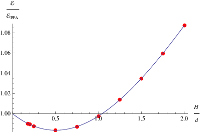
Results of the calculation for a strip parallel to a plane are shown in Fig. 1. We show the ratio of the full energy to the proximity force approximation, where the latter is given by
| (72) |
We also show a polynomial fit to this quantity, which shows good agreement with the expansion of Eq. (1),
| (73) |
from which we obtain and . These dimensionless quantities give edge corrections to the proximity force result: captures the effect of each of the two edges individually, while gives an interaction energy due to the combined effect of the two edges. The result for agrees with results obtained at lower precision in the case of a half-plane parallel to a plane [9, 10, 11, 23]. The strip allows for better numerical precision than the half-plane, because the leading proximity force term is a energy per unit length rather than an energy per unit area. (Of course, the subleading correction is not present in the half-plane case, since it has only a single edge.)
We can gain some qualitative insight into these corrections by considering the effects of edges on the fluctuation modes that contribute to the Casimir energy. The positive sign of indicates that the edge boundary condition suppresses fluctuations that would otherwise contribute to the attractive Casimir interaction (though this effect arises only from terms beyond the first reflection [9, 24, 23]), while the negative sign of indicates an enhancement of the Casimir energy due to the effect of one edge on the other: Some of the modes whose contribution would be suppressed by one edge have already been suppressed by the other edge, and so the combined effect of two edges reduces the Casimir energy by less than the sum of their individual contributions. We note that Eq. (63) is meromorphic around , so we cannot have a term proportional to in Eq. (1). In contrast, for an expansion at large , the essential singularity in the integrand of Eq. (63) makes it possible for such inverse logarithms to appear, and indeed the leading term at large distances is proportional to in that case [26].
V Acknowledgments
This work was supported in part by the National Science Foundation (NSF) through grant PHY-1213456. N. G. thanks G. Bimonte, T. Emig, R. L. Jaffe, M. Kardar, and M. Krüger for helpful conversations.
References
- [1] F. Alhargan, ACM T Math Software 26, 390 (2000a).
- [2] F. Alhargan, ACM T Math Software 26, 408 (2000b).
- [3] O. Kenneth and I. Klich, Phys. Rev. Lett. 97, 160401 (2006).
- [4] A. Lambrecht, P. A. Maia Neto, and S. Reynaud, New J. Phys. 8, 243 (2006).
- [5] A. Bulgac, P. Magierski, and A. Wirzba, Phys. Rev. D73, 025007 (2006).
- [6] T. Emig, N. Graham, R. L. Jaffe, and M. Kardar, Phys. Rev. Lett. 99, 170403 (2007).
- [7] S. J. Rahi, T. Emig, N. Graham, R. L. Jaffe, and M. Kardar, Phys. Rev. D80, 085021 (2009).
- [8] N. Graham, Phys. Rev. D87, 105004 (2013).
- [9] M. F. Maghrebi, S. J. Rahi, T. Emig, N. Graham, R. L. Jaffe, and M. Kardar, Proc. Nat. Acad. Sci. 108, 6867 (2011a).
- [10] N. Graham, A. Shpunt, T. Emig, S. J. Rahi, R. L. Jaffe, and M. Kardar, Phys. Rev. D81, 061701 (2010).
- [11] N. Graham, A. Shpunt, T. Emig, S. J. Rahi, R. L. Jaffe, and M. Kardar, Phys. Rev. D83, 125007 (2011).
- [12] H. Gies and K. Klingmuller, Phys. Rev. Lett. 97, 220405 (2006).
- [13] A. Weber and H. Gies, Phys. Rev. D80, 065033 (2009).
- [14] D. Kabat, D. Karabali, and V. Nair, Phys. Rev. D81, 125013 (2010a).
- [15] D. Kabat, D. Karabali, and V. Nair, Phys. Rev. D82, 025014 (2010b).
- [16] C. D. Fosco, F. C. Lombardo, and F. D. Mazzitelli, Phys. Rev. D84, 105031 (2011).
- [17] G. Bimonte, T. Emig, R. L. Jaffe, and M. Kardar, Europhys. Lett. 97, 50001 (2012).
- [18] L. Teo, Phys. Rev. D88, 045019 (2013), eprint 1303.5176.
- [19] N. W. McLachlan, Theory and application of Mathieu functions (Clarendon Press, Oxford, 1951).
- [20] M. Abramowitz and I. A. Stegun, Handbook of Mathematical Functions With Formulas, Graphs, and Mathematical Tables (U.S. government printing office, Washington, 1972).
- [21] P. M. Morse and H. Feshbach, Methods of Theoretical Physics (McGraw-Hill, New York, 1953).
- [22] Bateman manuscript project, Higher transcendental functions, vol. 1 (McGraw-Hill, New York, 1953).
- [23] M. F. Maghrebi and N. Graham, Europhys. Lett. 95, 14001 (2011).
- [24] M. F. Maghrebi, R. L. Jaffe, and R. Abravanel, Phys. Rev. D84, 061701 (2011b).
- [25] N. Graham and K. D. Olum, Phys. Rev. D72, 025013 (2005).
- [26] T. Emig, R. L. Jaffe, M. Kardar, and A. Scardicchio, Phys. Rev. Lett. 96, 080403 (2006).