The Private and Public Correlation Cost
of Three Random Variables with Collaboration
Abstract
In this paper we consider the problem of generating arbitrary three-party correlations from a combination of public and secret correlations. Two parties – called Alice and Bob – share perfectly correlated bits that are secret from a collaborating third party, Charlie. At the same time, all three parties have access to a separate source of correlated bits, and their goal is to convert these two resources into multiple copies of some given tripartite distribution . We obtain a single-letter characterization of the trade-off between public and private bits that are needed to achieve this task. The rate of private bits is shown to generalize Wyner’s classic notion of common information held between a pair of random variables. The problem we consider is also closely related to the task of secrecy formation in which is generated using public communication and local randomness but with Charlie functioning as an adversary instead of a collaborator. We describe in detail the differences between the collaborative and adversarial scenarios.
I Introduction
Three-party correlations are central objects of interest in the discussion of public key agreement [Mau93, AC93]. Two parties (Alice and Bob) have access to some source which generates multiple copies of three random variables . When copies are generated, Alice sees , Bob sees , and a third party (Charlie) sees . In the standard key agreement scenario, Charlie is viewed as untrustworthy eavesdropper and Alice and Bob wish to extract perfectly shared randomness from using local randomness and public communication (LOPC). The security constraint is that at the end of this protocol, Charlie should be almost completely uncorrelated from Alice and Bob’s shared randomness.
However, in many scenarios it may not be appropriate to assume that Charlie is a malicious eavesdropper. In fact, Charlie may actually be a helper or collaborator to Alice and Bob in their pursuit of obtaining private randomness from . For instance, one might imagine that Charlie represents some centralized hub that wishes to establish a secure link between two of its users. Distillation problems of this sort have been studied in Ref. [CN00]; see also Refs. [GW03, SVW05, Win07] for quantum analogues.
This paper considers the reverse of the scenario just described. Instead of asking how much secret key can be distilled from using LOPC, we ask how much secret key is needed to build using LOPC. This kind of problem has been studied much less, but goes back all the way to Wyner [Wyn75], and has received much more attention only in the last decade or so, from the Reverse Shannon Theorem [BSST02] (and its quantum generalization [B+14]), more generally to so-called coordination problems [Cuff08, Cuff09].
Whether Charlie is an adversary or collaborator greatly changes the nature of the problem, as we shall see. First consider when Charlie is a collaborator. Alice and Bob initially share perfect randomness that is secret from Charlie, and using LOPC, they generate public communication and variables . However, in the spirit of collaboration, the public communication which they generate should also be usable by Charlie to generate so that ultimately . We will refer to this as the collaborative model for generating . In a particular protocol, there will exist some trade-off between the amount of secret randomness Alice and Bob initially share versus the amount of public communication used to build . The main contribution of this paper is a single-letter characterization of this trade-off (Theorem 7).
On the other hand, when Charlie is an adversary, some care is needed to properly quantify the correlation costs of . This is because here Alice and Bob really only care about generating the marginal since, after all, Charlie is an adversary. Nevertheless, may contain some information about , and this should be somehow captured in the total cost for . In light of these considerations, Renner and Wolf have proposed the following notion of secrecy formation [RW03]. Starting from a source of pre-shared secret bits, Alice and Bob perform LOPC to generate three random variables , where again describes the public communication conducted during the protocol. With being the target distribution, the goal is for to be approximately equivalent to some joint random variables of the form , where is obtained by processing . This latter condition means that Charlie could simulate the entire communication Alice and Bob use to produce from his part . In the words of Renner and Wolf, this “formalizes the fact that the protocol communication observed by [Charlie] does not give him more information than .” We will refer to this as the adversarial model for generating .
In subsequent work, Horodecki et al. [HHHO05] discussed the hypothesis that the minimum rate of secret bits for generating in the adversarial sense is given by a quantity known as the intrinsic information [RW03]. If this were true, then optimal secrecy formation could alternatively be obtained by an asymptotic preparation of randomly chosen private correlations (i.e. distributions in which Charlie is completely uncorrelated from Alice and Bob). However, Horodecki et al. considered this hypothesis to be likely false, and indeed it was later shown to be so by one of us, with a single-letter secret key cost formula being derived [Win05]. In the present paper, we revisit the precise trade-off between public and secret correlation costs computed in Ref. [Win05] for the adversarial model, in particular the direct (achievability) part of the main result of that paper. Note that the direct part is also implicitly discussed in [HHHO05], since the formula of the secrecy cost is a convex hull over certain decompositions of the Alice-Bob distribution, decompositions characterized by Wyner’s common information [Wyn75]. The converse (lower bound) presented in [HHHO05, Prop. 1] however was incomplete as it assumed a property known as “asymptotic continuity” (cf. [HHHH09]) of the common information, which was shown to be false in Ref. [Win05]; see also Witsenhausen [Wit76]. The correct optimality proof required a much more complex argument [Win05].
Both the collaborative and adversarial models generalize Wyner’s notion of common information [Wyn75]. In Wyner’s scenario, Alice and Bob simply want to produce using pre-shared randomness with no additional communication. The minimum amount of randomness per copy needed to approximately simulate is what Wyner identifies as the common information held between and . This can be seen as a special case of the three-party problems when ranges over just a single value and the public communication rate is zero.
Interest in secrecy formation is largely inspired by the analogous notion of entanglement formation when dealing with quantum systems and quantum information. The entanglement cost of a quantum state is defined to be the asymptotic rate of pre-shared ebits that are needed to prepare many copies of the given state [HHT01]. In the quantum setting, a third party is not introduced into the definition of entanglement cost since by its very nature, quantum entanglement possesses an inherent shielding from external parties. This latter property is sometime referred to as the monogamy of entanglement [HHHH09].
The structure of this paper is as follows. We begin in Sect. II by describing how, for the task at hand, all public communication generated during an LOPC protocol can be equivalently replaced by pre-shared public correlations at the start of the protocol and no further communication. This provides a significant simplification to the problem since a general LOPC protocol can involve multiple rounds of communication. In Sect. III, we introduce in greater detail Wyner’s model for generating bipartite random variables as well as the tripartite models when Charlie is acting either as a collaborator or as an adversary. The main result of this paper is presented in Sect. IV and its proof is given in Sects. V and VI. The Appendix contains a reformulation of the original protocol given in [Win05].
Throughout this paper, random variables will be denoted by capital italic letters , etc. The values of the these variables will be written in lower-case , etc., and a sequence of such values will be denoted as , etc. The distribution of a given random variable will be interchangeably written by and . When variables and range over a common alphabet , their variational distance (up to a factor of ) is given by
Finally, when three random variables form a Markov chain, this will be denoted by , and it indicates that . Equivalently, its conditional mutual information satisfies .
II Replacing Public/Secret Communication by Shared Correlations
Consider a general LOPC protocol in which Alice and Bob begin with perfectly correlated bits. Specifically, Alice (resp. Bob) has variable (resp. ) such that and . Alice, Bob and Charlie may also have sources of local randomness, but these can be built directly into the local processing of the variables by allowing for stochastic mappings. The protocol will then involve a sequence of publicly announced messages where is a function of . Here, denotes all previous messages. At the end of the protocol, the entire communication can be represented by the variable . Alice and Bob then generate random variables and , both as the image of some stochastic map applied to . Thus, the entire protocol can be represented by random variables whose distribution satisfies
| (1) |
The particular distribution depends on the nature of the LOPC protocol, and here we are using the fact that the computations of and are done locally (i.e. independently of each other). In the collaborative model, Charlie also obtains as a function of , and the distribution is given by
| (2) |
Hence to simulate the random variables with no communication, it suffices for all three parties to first share the random variable (which represents the public correlations of the protocol); additionally, Alice and Bob share the variable (representing the secret correlations of the protocol). Conversely, to each distribution , an LOPC protocol exists with Alice and Bob first sharing secret bits and then broadcasting according to .
Remark 1
In the next section, we introduce models in which and are uncorrelated. While this does not correspond directly to the most general LOPC process, when proving the converse in Section V, we will allow for correlated and . Hence, the upper bound we derive on secret and public correlation rates will also hold in the LOPC scenario. In Section VI, we show that these lower bounds can be obtained by public and private correlations and which are, in fact, independent.
Alternatively, one can also directly show, by an operational argument, that protocols with correlated and can always be asymptotically simulated by one where public and secret correlation are independent.
III Three Models of Correlation Generation
We now describe three different models for generating dependent random variables. While both the models in Sects. III-A and III-B have been well-studied, our new contribution is the model described in Sect. III-C.
III-A Wyner’s Common Information

In this subsection, we review Wyner’s notion of common information as well as one of its operational interpretations [Wyn75].
Definition 2 (Wyner [Wyn75])
The common information between two random variables and with joint distribution is defined as
| (3) |
where the minimization is taken over all triples of random variables so that
- •
the marginal distribution for is ;
- •
forms a Markov chain.
Furthermore, the minimum in Eq. (3) can be obtained with a random variable ranging over sets of size no greater than .
To see why this quantity might capture the notion of “common information” between and , consider the following task. Alice and Bob have access to a common source , and acting independently of one another, they wish to process in different ways so that their final joint distribution is a many-copy approximation of the target distribution (see Fig. 1). The common information is the minimum rate of common randomness needed to perform this task.
More precisely, we define an source synthesis code to consist of the following:
- •
a set with cardinality ;
- •
conditional probability distributions and , , on , respectively;
such that
where
| (4) |
We say the rate is achievable if for all and sufficiently large there exists a source synthesis code . Define the correlation cost of as .
Theorem 3 (Wyner [Wyn75])
For any pair of random variables, the minimum achievable rate of a source synthesis code is given by the common information:
The key ingredient in Wyner’s achievability construction is a general result saying that for any two random variables and , the distribution of can be reliably simulated by sampling from approximately sequences among the range of and then applying the channel (see Lemma 12 below). Hence if with satisfying , then this simulation can be done locally, as depicted and in Fig. 1 and described in Eq. (4). This construction need not be limited to only two parties. For example, one can analogously define the common information of three variables with distribution as
| (5) |
where the minimization is taken over all variables so that
- •
the marginal distribution for is ;
- •
are conditionally independent variables given .
Operationally, and in complete analogy to Wyner’s Theorem 3, is the smallest rate of shared random bits that are needed to generate when Alice, Bob and Charlie independently process . In other words, there are now three channels , and so that
with , for arbitrarily small . This is a special case of the more general three-party collaborative scenario that we will study below. Specifically, when the wires connected to are removed in Fig. 3, we recover this scenario of Wyner’s common information for three parties.
III-B Key Cost in Three-Party Adversarial Scenario

We now consider three-party distributions generated by two sources of correlations. First is the adversarial model where Charlie is considered to be a malicious eavesdropper. Again, let be the distribution whose correlation costs we wish to quantify. In the adversarial model, Alice and Bob start with some initially perfectly correlated bits that are secret from Charlie. Using LOPC, they wish to generate many copies of so that the total public communication produced in the protocol gives Charlie no more information about than what he has in the distribution . In other words, Charlie is able to apply some local processing on her share part of so that the resulting distribution is close to the distribution generated in the LOPC protocol. There will be some trade-off between the amount of initial secret correlations and the amount of public communication consumed in the protocol. Intuitively, the more perfectly correlated secret bits that Alice and Bob initially share, the less public communication they will need to generate .
By the discussion in Sect. II, we can simulate the entire protocol having public communication by a protocol with no communication but initially shared public correlations. The resulting scenario is depicted in Fig. 2. The trade-off between public and private correlations in the task of secrecy formation is formally defined as follows.
Definition 4 (Renner & Wolf [RW03])
For distribution , an secrecy formation code is composed of the following:
- •
random variables having joint distribution over the set with cardinalities and respectively;
- •
conditional distributions on and ,
which generate random variables with joint distribution
- •
a channel such that
(6)
The rate pair is achievable if, for all , we can find an sufficiently large such that there exists a secrecy formation code .
The public-vs-secret tradeoff function is
and the secret key cost of the triple is
Theorem 5 (Winter [Win05])
For the secrecy formation of the distribution , the rate pair is achievable iff there exist random variables such that
| (7) |
where the random variables satisfy the properties
- 1.
The marginal distribution is ;
- 2.
The following Markov chains hold:
(8)
Furthermore the auxiliary random variables w.l.o.g. have bounded ranges: and .
In particular,
is the secret key cost of with unlimited public communication. ∎
III-C Key Cost in Three-Party Collaborative Scenario
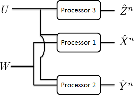
We now shift perspectives and view Charlie as a collaborator instead of an adversary. As such, for a given distribution , Alice and Bob are no longer content with just generating variables using LOPC that are close to the target variables . They also want the public communication to be sufficiently correlated with so that Charlie can locally process to jointly produce dependent variables that are close to . Like in the adversarial setting, the public communication can be replaced with initially shared correlations between all the parties (see Fig. 3). There will also be a trade-off between public and private correlations in the following sense.
Definition 6
For a given tripartite probability distribution over , we define an split-source synthesis code to be composed of the following:
- •
sets and with cardinalities and , respectively;
- •
conditional probability distributions on , and ,
which generate random variables with joint distribution
(9)
such that .
The rate pair is achievable if, for all , we can find an sufficiently large such that there exists a split-source synthesis code .
IV Statement of Results
In this section we present our main result: a single-letter characterization of the trade-off between the public and private correlation rate pair in the collaborative scenario of Sect. III-C.
Theorem 7
For the split-source synthesis of the distribution , the rate pair is achievable iff there exist random variables such that
| (10) |
where all random variables satisfy the following properties
- 1.
The marginal distribution is ;
- 2.
and form Markov chains.
Furthermore, the random variables and in Eq. (10) can be restricted to sets of size no greater than and , respectively.
Fig. 4 illustrates the two-dimensional achievable rate region for the collaborative synthesis of a tripartite distribution. Theorem 7 determines the nontrivial corner point in Fig. 4: indeed, the public correlation rate at is given precisely by , the Wyner common information between and . Another corner point is when : here, the problem reduces to the three-party Wyner common information as described in Sect. III-A. Hence, the public correlation rate at is given by . From this we see that Theorem 7 generalizes the notion of Wyner’s common information (Theorem 3) when is trivial.

Any rate pair on the line connecting with can be achieved by time-sharing the two protocols that achieve and , respectively. What can be said about this line connecting and ? Denote the rate pairs at these points by and respectively. Since , the slope of the connecting line will always be negative. On the other hand, since the secret correlations of any protocol can always be converted to public correlations, we have that the
| (11) |
Hence the boundary line connecting and must have a slope not exceeding . For some distributions, Eq. 11 is an equality while for others it is not. In the latter cases, the optimal exchange between private and public correlations is nontrivial and not a simple publication of the private correlations.
Example 1: Let be any distribution such that , i.e. is a function of . Then it is easy to verify that the optimal and tradeoff is one-to-one, and thus the line connecting and has a slope of . First consider the point . Here the public correlation rate is given by such that . It is easy to show that , and this lower bound can be attained by since . Therefore, and where . Let denote the variable attaining this minimum. Now consider the point where and such that are conditionally independent given . Then
| (12) |
where the first inequality is data processing since ; the second inequality is obtained since if are conditionally independent given , then ; and the last equality follows because . Combining with Eq. (11), we see that
Example 2: Next, we consider a very simple distribution over with the only nonzero values being for with and with . This belongs to a more general class of “L-shaped” distributions studied by Witsenhausen [Wit76, Thm. 7]. From his result, the common information is found to be
| (13) |
This is computed from the optimal decomposition of into conditionally independent parts:
Here we have grouped into one variable ranging over so that the element of the matrix is . From this decomposition, we see that
| (14) |
For the corner point , we observe that are conditionally independent given . Hence,
| (15) |
Hence,
| (16) |
and so the optimal private to public exchange for this distribution is not achieved by simply publicly revealing private correlations.
V Converse
Here we derive lower bounds that hold for more general models than a synthesis code. Specifically, we assume that is given along with conditional probabilities , , and such that the generated distribution
| (17) |
satisfies . Note that the local processing in the secrecy formation protocol imposes that and form Markov chains. However, unlike a synthesis code defined in Sect. III-C, we do not require that and are independent. This relaxation enables to simulate LOPC protocols as discussed in Remark 1.
Following the argument in [Win05], monotonicity and the chain rule allow us to write
| (18) |
where is a uniformly distributed variable and the last equality follows from the conditional independence (see Proposition 8 below). We next introduce the following random variables and and the variables , , , , and defined through the joint distributions
| (19) |
Then
| (20) |
At the same time, applying the triangle inequality to allows us to conclude that
| (21) |
and therefore . Combining the latter with Eqns. (20) and (21) yields
| (22) |
Since are i.i.d., the marginal distribution of is . Hence, the previous inequality gives
| (23) |
Eq. (19) also gives that and . The Markov conditions , , and therefore imply
| (24) |
where .
From Eq. (19), we have which further implies that since , again by Eq. (19). Thus, for each fixed value of , we have that
Multiply both sides by and take the sum. Using the fact that and the triangle inequality lead to:
hence,
| (25) |
By the same arguments, we can bound the public communication as
To bound the term , we recall a well-known continuity relation: Any two random variables and ranging over with satisfy [CK11]. Therefore, using Eq. (22) and the fact that , we readily obtain
| (26) |
At this point we have constructed random variables that satisfy Eqns. (23)–(26). By Lemma 9, we can assume without loss of generality that and range over sets of size no greater than . Hence, the set of random variables satisfying Eqns. (23)–(26) is compact, and therefore a limit point will exist which also satisfies these constraints when taking . This proves the lower bound of Theorem 7. ∎
Proposition 8
If -part random variables and satisfy , then the reduced variables and satisfy for any , where and likewise .
Proof:
Consider the marginal distribution . Then
| (27) | ||||
Therefore, . ∎
Lemma 9
Suppose that are random variables with ranging over such that and . Then there exists random variables satisfying the same Markov chain and
| (28a) | ||||
| (28b) | ||||
| (28c) | ||||
with and ranging over sets and of sizes and . Furthermore, if also holds, then the size of can be further reduced to .
Proof:
For the given distribution , let and be the associated conditional distributions. For each fixed , let be the collection of conditional distributions over such that if . This represents a total of linear constraints on the (note if also holds, then reduces to which represents a total of linear constraints on the ). Now is convex and the set will obtain both its maximum and minimum at an extreme point of . Then an application of Carathéodory’s Theorem (Lemma 10) guarantees that such an extreme point is a distribution over with no more than nonzero probability values [Kle63]. Hence by a conditional relabeling of the , we have a subset with and a collection of conditional distributions over such that
| (29a) | ||||
| (29b) | ||||
We now perform a similar argument by letting be the set of all distributions over such that if
and . This represents linear constraints on , and we seek the minimum value of the set . A second application of Carathéodory’s Theorem ensures the existence of a distribution ranging over with for which
| (30a) | ||||
| (30b) | ||||
| (30c) | ||||
This completes the construction of random variables whose joint distribution is given by . By its definition and by Eq. (29a), inherits whatever Markov chain properties are present in . Eq. (30a) gives , and combining this with Eq. (30b) yields . Finally, combining Eq. (30c) and Eq. (29b) gives
| (31) |
concluding the proof. ∎
Lemma 10 (Carathéodory’s Theorem [Roc96])
Let be a subset of and its convex hull. Then any can be expressed as a convex combination of at most elements of . ∎
Remark 11
An application of Carathéodory’s Theorem shows that if the elements of are further required to satisfy linear constraints, then the resulting set is convex with extreme points being convex combinations of at most extreme points of [Kle63].
VI Achievability
Let be random variables with joint distribution satisfying (1) and (2) and . In what follows, we let denote the set of all -typical sequences with respect to random variable having distribution . Recall that a sequence is -typical if for all [CK78].
Our code makes repeated use of Wyner’s original code. The following is proven in [Wyn75], where here we have modified the statement using Pinsker’s inequality, , to obtain a bound on the variational distance. See also later works by Han and Verdú [HV92, HV93] and Ahlswede [A06], where more general versions were proved (Ref. [AW02] contains a quantum analogue).
Lemma 12 (Wyner [Wyn75, Thm. 6.3])
Let be random variables over with joint distribution , and let . For and sufficiently large , there exists a subset of size such that for
| (32) |
it holds that .
Identify and in Lemma 12. Thus, for sufficiently large, we can find a subset such that with
| (33) |
and
| (34) |
where we have used the Markov chain . Here, will be the encoder employed by the collaborative third party.
We next consider the term
| (35) |
where is a sequence of length that occurs with the event . Knowing that , we let , and for each , we apply Lemma 12 on the conditional distribution with the choice and . This will generate a collection of codeword sets , each with respective size . Furthermore,
| (36) |
satisfies . In the previous equation, the Markov chain has been employed. For each and , let denote the marginal distribution obtained from by summing over the last events. Let be defined likewise. Thus,
where
| (37) |
We now paste together the different codes to form the code set . For any typical and , we define the local generators
| (38) |
which satisfy
| (39) |
The size of is bounded by
| (40) |
Combining this simulation of with Eq. (34) gives the final error bound
| (41) |
where
Since and , the bounds on , and can be made arbitrarily close to , and zero, respectively.
∎
VII Conclusion
In this paper we have introduced the problem of tripartite correlation generation using public and private correlations. This can be seen as a collaborative alternative to the cryptographic problem of secrecy formation. We have found that despite the two different natures of the problem, the optimal secret correlation rates have a very similar structure. We have completely characterized the public-vs-private rate region for the collaborative scenario. One point of interest is when the public correlation rate is minimum (point in Fig. 4), and another is when the secret correlation rate is zero (point in Fig. 4). We have shown that the optimal exchange of private to public correlations does not always involve a trivial publicizing of private information. However, it is an interesting open problem to determine the slope of the line connecting and for a general distribution, in particular to understand what limits there are, if any, on the exchange rate of private to public correlation rate.
Further afield, following the example of Ref. [Win05], one could ask for the benefit of using entanglement instead of, or in addition to, the private and public shared randomness. We leave this and other questions for future investigations.
Acknowledgments
EC was supported by the National Science Foundation (NSF) Early CAREER Award No. 1352326. MH is supported by an ARC Future Fellowship under Grant FT140100574. AW was supported by the European Commission (STREP “RAQUEL”), the European Research Council (Advanced Grant “IRQUAT”), and the Spanish MINECO (project FIS2008-01236) with FEDER funds.
Appendix A Achievability Proof of Secret Key Cost in the Adversarial Scenario
Here we review the achievability component of Theorem 5. The coding for Alice and Bob is the same as described in Section VI. Let be random variables obtaining the minimum in Theorem 5, and let denote their joint distribution so that the marginal on is . The public correlation (communication) is ( i.i.d. realisations of ). Let us restrict attention to the typical subset for which the relative frequency of each letter in is close to ; in particular, . For the set of positions where occurs, we can employ Lemma 12.
Consider and in Lemma 12. Thus for sufficiently large, we can find a subset such that with
| (42) |
where
We paste these codes together and define local channels for Alice and Bob which, for each , samples from the concatenated code and discards the extra letter occurrences not found in (see Section VI). With denoting the set of code words, this generates the simulation
which satisfies
| (43) |
The size of is bounded by
| (44) |
Charlie’s Simulation: Eq. (43) holds for every . The next question is how we choose our code words , which represents the public communication. If we just took as the codebook, then the public correlation rate would be . But we can actually do better, and we will use Wyner’s theorem again to construct a smaller codebook.
From Wyner, for sufficiently large there exists a subset with such that
and
| (45) |
Let be uniformly distributed over and define the channel by
| (46) |
When Charlie applies to his part of distribution , the new distribution is given by
| (47) |
Note that the reduced distribution is precisely what is obtained when Charlie attempts to simulate the public communication by acting on with . Thus, we want to prove that is close to the distribution generated by when is chosen uniformly from , which we denote by
To do this, we first bound the difference
| (48) |
Here, we have used both Eqns. (46) and (45), and the last line follows from the Markov chain condition . Therefore, combining with Eq. (43), we obtain the desired result that
| (49) |
To summarize the protocol, consider any and sufficiently large. Either Alice or Bob locally generates the random variable which is uniformly distributed over a set of size . The value of is announced publicly. Sharing no more than bits of secret correlation, Alice and Bob generate distribution which is jointly distributed with according to . At the same time, we have shown the existence of a channel such that when Charlie applies this to her part of , it generates the distribution for which
Therefore, we have satisfied the two components of the achievability criteria.
References
- [A06] Rudolf Ahlswede. On Concepts of Performance Parameters for Channels. In General Theory of Information Transfer and Combinatorics (R. Ahlswede, L. Bäumer, N. Cai, H. Aydinian, V. Blinovsky, C. Deppe, and H. Mashurian, eds.), Lecture Notes in Computer Science, vol. 4123, pp. 639-1¤7663, Springer Verlag, Berlin Heidelberg, 2006.
- [AC93] Rudolf Ahlswede and Imre Csiszár. Common Randomness in Information Theory and Cryptography. I. Secret Sharing. IEEE Transactions on Information Theory 39(4):1121–1132, 1993. doi:10.1109/18.243431.
- [AW02] Rudolf Ahlswede and Andreas Winter. Strong converse for identification via quantum channels. IEEE Transactions on Information Theory, 48(3):569-1¤7579, 2002.
- [BSST02] Charles H. Bennett, Peter W. Shor, John A. Smolin, and Ashish V. Thapliyal. Entanglement-assisted capacity of a quantum channel and the reverse Shannon theorem. IEEE Transactions on Information Theory 48(10):2637–2655, 2002.
- [B+14] Charles H. Bennett, Igor Devetak, Aram W. Harrow, Peter W. Shor, and Andreas Winter The Quantum Reverse Shannon Theorem and Resource Tradeoffs for Simulating Quantum Channels. IEEE Transactions on Information Theory 60(5):2926–2959, 2014.
- [CK78] Imre Csiszár and Janos Körner. Broadcast channels with confidential messages. IEEE Transactions on Information Theory 24(3):339–348, 1978. doi:10.1109/TIT.1978.1055892.
- [CK11] Imre Csiszár and Janos Körner. Information Theory: Coding Theorems for Discrete Memoryless Systems. Second ed., Cambridge University Press, Cambridge, UK, 2011.
- [CN00] Imre Csiszár and Prakash Narayan. Common randomness and secret key generation with a helper. IEEE Transactions on Information Theory 46(2):344–366, 2000. doi:10.1109/18.825796.
- [Cuff08] Paul Cuff. Communication Requirements for Generating Correlated Random Variables. In Proceedings of the International Symposium on Information Theory, ISIT 2008, pp. 1393–1397, Toronto, Canada, 6-11 July 2008.
- [Cuff09] Paul Cuff. Communication in Networks for Coordinating Behaviour. PhD thesis, Stanford University, 2009.
- [GW03] Matteo Gregoratti and Reinhard F. Werner. Quantum lost and found. Journal of Modern Optics 50(6&7):913–933, 2003.
- [HV92] Te-Sun Han and Sergio Verdú. New Results in the Theory of Identification via Channels. IEEE Transactions on Information Theory 38(1):141¤7-25, 1992
- [HV93] Te-Sun Han and Sergio Verdú. Approximation Theory of Output Statistics. IEEE Transactions on Information Theory 39(3):7521¤7-772, 1993.
- [HHT01] Patrick M. Hayden, Michał Horodecki, and Barbara M. Terhal. The asymptotic entanglement cost of preparing a quantum state. Journal of Physics A: Mathematical and General 34(35):6891–6898, 2001.
- [HHHH09] Ryszard Horodecki, Paweł Horodecki, Michał Horodecki, and Karol Horodecki. Quantum entanglement. Reviews in Modern Physics 81(2):865, 2009. doi:10.1103/RevModPhys.81.865.
- [HHHO05] Karol Horodecki, Michał Horodecki, Paweł Horodecki, and Jonathan Oppenheim. Information theories with adversaries, intrinsic information, and entanglement. Foundations of Physics 35(12):2027–2040, 2005. doi:10.1007/s10701-005-8660-5.
- [Kle63] Victor Klee. On a theorem of Dubins. Journal of Mathematical Analysis and Applications 7(3):425–427, 1963. doi:10.1016/0022-247X(63)90063-5.
- [Mau93] Ueli M. Maurer. Secret Key Agreement by Public Discussion From Common Information. IEEE Transactions on Information Theory 39(3):733–742, 1993. doi:10.1109/18.256484.
- [Roc96] R. Tyrell Rockafellar. Convex Analysis. Princeton Mathematical Series. Princeton University Press, 1996.
- [RW03] Renato Renner and Stefan Wolf. New bounds in secret-key agreement: The gap between formation and secrecy extraction. In Proceedings of Advances in Cryptology, EUROCRYPT 2003 (Eli Biham, ed.), Lecture Notes in Computer Science, vol. 2656, pp. 562–577. Springer Verlag, Berlin Heidelberg, 2003. doi:10.1007/3-540-39200-9_35.
- [SVW05] John A. Smolin, Frank Verstraete, and Andreas Winter. Entanglement of assistance and multipartite state distillation. Physical Review A 72:052317, 2007.
- [Win05] Andreas Winter. Secret, public and quantum correlation cost of triples of random variables. In Proceedings of the International Symposium on Information Theory, ISIT 2005, pp. 2270–2274, Adelaide, South Australia, 5-9 September 2005 doi:10.1109/ISIT.2005.1523752.
- [Win07] Andreas Winter. On Environment-Assisted Capacities of Quantum Channels. Markov Processes and Related Fields 13(1-2):297–314, 2007.
- [Wit76] Hans S. Witsenhausen. Values and bounds for the common information of two discrete random variables. SIAM Journal of Applied Mathematics 31:313–333, 1976. doi:10.1137/0131026.
- [Wyn75] Aaron D. Wyner. The Common Information of Two Dependent Random Variables. IEEE Transactions on Information Theory 21(2):163–179, 1975. doi:10.1109/TIT.1975.1055346.