Constraining double parton correlations and interferences

The color structure of the double quark distributions in (2) can be parametrized as [6]

$\displaystyle F_{jj^{\prime},kk^{\prime}}=\frac{1}{N_{c}^{2}}\left[{}^{1\hskip-1.00374pt}F\;\delta_{jj^{\prime}}\delta_{kk^{\prime}}+\frac{2N_{c}}{\sqrt{N_{c}^{2}-1}}\,^{8\hskip-1.00374pt}F\;t^{a}_{jj^{\prime}}t^{a}_{kk^{\prime}}\right],$

(6)

where the unprimed indices $j,k$ corresponds to the quark in the amplitude entering the first and second hard interaction, while primed indices refers to the conjugate amplitude, as in figure 1.

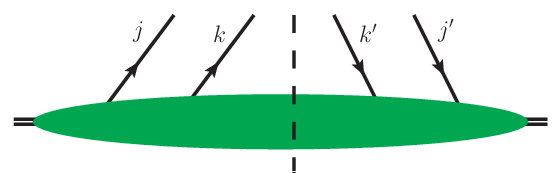
${}^{1\hskip-1.00374pt}F$ describe the distribution when the quark fields taking part in the same hard interaction form a color singlet, while ${}^{8\hskip-1.00374pt}F$ describes the color octet interference contribution between the two hard interactions. The interference term couples the two quark fields in the same hard interaction in a color $SU(3)$ octet. The normalization of the interference distribution is chosen such that the two distributions enter with equal weight in the cross section for the production of a color singlet. With this choice the size of the two distributions directly indicates their phenomenological importance. For quark-antiquark (antiquark-quark) distributions the $k$ and $k^{\prime}$ ($j$ and $j^{\prime}$) indices in (6) are interchanged. For DPDs with one quark and one antiquark the color structure is different and we will return to these distributions when discussing fermion-number interference in section III.3.

Taking the three possible colors for the quarks ${r,g,b}$ and organizing the singlet and octet correlation distributions into a color-density matrix where the columns (rows) are given by the color of the two quarks in the (conjugate-) amplitude we could use the property of (5) to set limits on the color correlations. However, such a representation is reducible and we consider instead the two irreducible representations of two quarks in the product representation $3\otimes 3=\bar{3}\oplus 6$, i.e. in an anti-triplet and a sextet representation, diagonalizing the color density matrix.

Using a recoupling, the color anti-triplet and sextet distributions can be expressed in terms of the color square ${}^{1\hskip-1.00374pt}F$ and correlation ${}^{8\hskip-1.00374pt}F$ distributions by using projection operators [26] $(\delta_{jj^{\prime}}\delta_{kk^{\prime}}\pm\delta_{jk^{\prime}}\delta_{kj^{\prime}})$, where the minus (plus) sign gives the anti-triplet (sextet). The resulting relations reads

$\displaystyle F^{(\bar{3})}_{qq}$

$\displaystyle=\frac{1}{N_{c}^{2}}\left({}^{1\hskip-1.00374pt}F_{qq}-\frac{N_{c}+1}{\sqrt{N_{c}^{2}-1}}\,^{8\hskip-1.00374pt}F_{qq}\right),$

$\displaystyle F^{(6)}_{qq}$

$\displaystyle=\frac{1}{N_{c}^{2}}\left({}^{1\hskip-1.00374pt}F_{qq}+\frac{N_{c}-1}{\sqrt{N_{c}^{2}-1}}\,^{8\hskip-1.00374pt}F_{qq}\right),$

(7)

where we have chosen the normalization with respect to the ${}^{1\hskip-1.00374pt}F_{qq}$ distribution. We will throughout this paper use the notation with a superscript following the distribution $F^{(R)}$ in order to denote the distribution in which the two partons in the amplitude couple to the $SU(3)$ representation $R$. This must not be confused with ${}^{R\hskip-1.00374pt}F$, where the representation $R$ is formed by one field in the amplitude and one in the conjugate amplitude. Up to overall normalization, equivalent equations can be obtained by making use of unitary $SU(3)$ color recouping matrices [27, 28]. The interpretation of $F_{qq}^{(\bar{3})}$ and $F_{qq}^{(6)}$ as describing probabilities for finding two quarks in definite color states gives the upper bounds on the color interference DPDs

${}^{1\hskip-1.00374pt}F_{qq}$

$\displaystyle\geq\frac{N_{c}+1}{\sqrt{N_{c}^{2}-1}}\,^{8\hskip-1.00374pt}F_{qq},$

${}^{1\hskip-1.00374pt}F_{qq}$

$\displaystyle\geq-\frac{N_{c}-1}{\sqrt{N_{c}^{2}-1}}\,^{8\hskip-1.00374pt}F_{qq}.$

(8)

These bounds apply also when both quarks are replaced by antiquarks. The bounds agree with the results found in [5] when the difference in normalization of the interference distribution (${}^{8\hskip-1.00374pt}F$) is taken into account.

Specifying the flavor structure of the DPDs in equation (2) gives, for example, the flavor squared distribution of an up and a down quark

$\displaystyle F_{ud}=2p^{+}\int\frac{dz^{-}_{1}}{2\pi}\,\frac{dz^{-}_{2}}{2\pi}\,dy^{-}\;e^{i\mskip 1.5mu(x_{1}z_{1}^{-}+x_{2}z_{2}^{-})\mskip 1.5mup^{+}}\left<p|\,(\bar{u}\;\Gamma_{q}\,u)(\bar{d}\;\Gamma_{q}\,d)\,|p\right>\,,$

(9)

while the corresponding flavor interference distribution is defined by

$\displaystyle F^{I}_{ud}=2p^{+}\int\frac{dz^{-}_{1}}{2\pi}\,\frac{dz^{-}_{2}}{2\pi}\,dy^{-}\;e^{i\mskip 1.5mu(x_{1}z_{1}^{-}+x_{2}z_{2}^{-})\mskip 1.5mup^{+}}\left<p|\,(\bar{u}\;\Gamma_{q}\,d)(\bar{d}\;\Gamma_{q}\,u)\,|p\right>\,.$

(10)

Limiting ourselves to the first three quark flavors $u$, $d$ and $s$ we construct the flavor-density matrix

$\displaystyle\begin{pmatrix}F_{dd}&0&0&0&0&0&0&0&0\\[5.69046pt] 0&F_{du}&0&F^{I}_{ud}&0&0&0&0&0\\[5.69046pt] 0&0&F_{ds}&0&0&0&F^{I}_{sd}&0&0\\[5.69046pt] 0&F^{I}_{du}&0&F_{ud}&0&0&0&0&0\\[5.69046pt] 0&0&0&0&F_{uu}&0&0&0&0\\[5.69046pt] 0&0&0&0&0&F_{us}&0&F^{I}_{su}&0\\[5.69046pt] 0&0&F^{I}_{ds}&0&0&0&F_{sd}&0&0\\[5.69046pt] 0&0&0&0&0&F^{I}_{us}&0&F_{su}&0\\[5.69046pt] 0&0&0&0&0&0&0&0&F_{ss}\end{pmatrix},$

(11)

where the columns (rows) correspond to the flavors of the two quarks in the (conjugate) amplitude, i.e. $dd$, $du$, $ds$, $ud$, $uu$, $us$, $sd$, $su$ and $ss$. Due to the positive semi-definiteness of the matrix (5) the principal minors of the two-dimensional subspaces gives

$\displaystyle F_{ab}F_{ba}\geq F^{I}_{ab}F^{I}_{ba},$

(12)

while the positivity of the eigenvalues leads to the constraints on the flavor interference

$\displaystyle F_{ab}+F_{ba}\pm\sqrt{(F_{ab}-F_{ba})^{2}+4F^{I}_{ab}F^{I}_{ba}}\geq 0.$

(13)

For mixed quark-antiquark distributions there can be flavor interference when the quark and antiquark are of the same flavor (i.e. $d\bar{d}$, $u\bar{u}$ or $s\bar{s}$). The flavor density matrix for quark-antiquark distributions reads

$\displaystyle\begin{pmatrix}F_{d\bar{d}}&0&0&0&F^{I_{d}}_{u\bar{u}}&0&0&0&F^{I_{d}}_{s\bar{s}}\\[5.69046pt] 0&F_{d\bar{u}}&0&0&0&0&0&0&0\\[5.69046pt] 0&0&F_{d\bar{s}}&0&0&0&0&0&0\\[5.69046pt] 0&0&0&F_{u\bar{d}}&0&0&0&0&0\\[5.69046pt] F^{I_{u}}_{d\bar{d}}&0&0&0&F_{u\bar{u}}&0&0&0&F^{I_{u}}_{s\bar{s}}\\[5.69046pt] 0&0&0&0&0&F_{u\bar{s}}&0&0&0\\[5.69046pt] 0&0&0&0&0&0&F_{s\bar{d}}&0&0\\[5.69046pt] 0&0&0&0&0&0&0&F_{s\bar{u}}&0\\[5.69046pt] F^{I_{s}}_{d\bar{d}}&0&0&0&F^{I_{s}}_{u\bar{u}}&0&0&0&F_{s\bar{s}}\end{pmatrix},$

(14)

where $F_{a\bar{a}}^{I_{b}}$ labels the distribution with $a\bar{a}$ in the amplitude and $b\bar{b}$ in the conjugate amplitude. The principal minors of the two dimensional subspaces give the bounds on the interference distributions,

$\displaystyle F_{a\bar{a}}F_{b\bar{b}}\geq F_{a\bar{a}}^{I_{b}}F_{b\bar{b}}^{I_{a}}.$

(15)

The most stringent bounds are given by the eigenvalues, which for the distributions where the quark and antiquark are of different flavors are simply the distributions (on the diagonal in the density matrix) themselves (there are no flavor interference for these distributions). For the distributions with quark-antiquark of equal flavor the eigenvalues result in rather complicated expressions, and there is little gain in giving them explicitly.

The bounds derived in this section are the first indication on the allowed size of the flavor interference DPDs and therewith their effect in DPS cross sections.

For distributions with one quark and one anti-quark, there can further be interferences in fermion-number, i.e. between quarks and anti-quarks. These are always accompanied by color interference - since two quarks cannot couple to a color singlet. Therefore, in order to set limits on DPDs with a quark and an antiquark we consider the joint space of color and fermion-number.

The DPDs describing interference in fermion-number between quarks and antiquarks are defined by [6]

	$\displaystyle I_{q_{1}\bar{q}_{2}}(x_{1},x_{2},\boldsymbol{y})$	$\displaystyle=2p^{+}\int\frac{dz^{-}_{1}}{2\pi}\,\frac{dz^{-}_{2}}{2\pi}\,dy^{-}\;e^{i\mskip 1.5mu(x_{1}z_{1}^{-}+x_{2}z_{2}^{-})\mskip 1.5mup^{+}}$
		$\displaystyle\quad\times\left<p|\,\bar{q}_{2}\bigl({\textstyle\frac{1}{2}}z_{2}\bigr)\,{\textstyle\frac{1}{2}}\gamma^{+}\,q_{1}\bigl(y-{\textstyle\frac{1}{2}}z_{1}\bigr)\bar{q}_{2}\bigl(-{\textstyle\frac{1}{2}}z_{2}\bigr)\,{\textstyle\frac{1}{2}}\gamma^{+}\,q_{1}\bigl(y+{\textstyle\frac{1}{2}}z_{1}\bigr)\,|p\right>\,,$		(16)

and the color structure can be decomposed as

$\displaystyle I_{jj^{\prime},kk^{\prime}}=\frac{1}{N_{c}^{2}}\left({}^{1\hskip-1.00374pt}I\delta_{jk^{\prime}}\delta_{j^{\prime}k}+\frac{2N_{c}}{\sqrt{N_{c}^{2}-1}}\,^{8\hskip-1.00374pt}It^{a}_{jk^{\prime}}t^{a}_{j^{\prime}k}\right).$

(17)

As in the quark-quark case above we start by going to an irreducible representation, this time in terms of a singlet and an octet distributions $3\otimes\bar{3}=1\oplus 8$. The quark-antiquark color density matrix reads

$\displaystyle\begin{pmatrix}F^{(1)}_{q\bar{q}}&0\\[5.69046pt] 0&F^{(8)}_{q\bar{q}}\end{pmatrix}.$

(18)

The color singlet and octet distributions can be expressed in terms of ${}^{1\hskip-1.00374pt}F$ and the interference distribution ${}^{8\hskip-1.00374pt}F$ as

$\displaystyle F^{(1)}_{q\bar{q}}$

$\displaystyle=\frac{1}{N_{c}^{2}}\left({}^{1\hskip-1.00374pt}F_{q\bar{q}}+\sqrt{N_{c}^{2}-1}\,^{8\hskip-1.00374pt}F_{q\bar{q}}\right)\geq 0,$

$\displaystyle F^{(8)}_{q\bar{q}}$

$\displaystyle=\frac{1}{N_{c}^{2}}\left({}^{1\hskip-1.00374pt}F_{q\bar{q}}-\frac{1}{\sqrt{N_{c}^{2}-1}}\,^{8\hskip-1.00374pt}F_{q\bar{q}}\right)\geq 0$

(19)

and their positivity leads to upper limits on the color correlations between the quark and antiquark. The inequalities hold true when interchanging $q$ and $\bar{q}$. The relations between $I^{(1)}$, $I^{(8)}$ and ${}^{1\hskip-1.00374pt}I$, ${}^{8\hskip-1.00374pt}I$ are equal to (19) with $F$’s replaced by $I$’s, but as they are interference distributions they do not have to be positive. Considering next the joint space of color and fermion number, we can extend the two $2\times 2$ matrices into a joint color-flavor number density matrix where the columns (rows) correspond to the color representations and fermion numbers of the first and second parton in the (conjugate) amplitude, i.e. $q\bar{q}$ singlet, $q\bar{q}$ octet, $\bar{q}q$ singlet, $\bar{q}q$ octet,

$\displaystyle\begin{pmatrix}F^{(1)}_{q\bar{q}}&0&I^{(1)}_{\bar{q}q}&0\\[5.69046pt] 0&F^{(8)}_{q\bar{q}}&0&I^{(8)}_{\bar{q}q}\\[5.69046pt] I^{(1)}_{q\bar{q}}&0&F^{(1)}_{\bar{q}q}&0\\[5.69046pt] 0&I^{(8)}_{q\bar{q}}&0&F^{(8)}_{\bar{q}q}\end{pmatrix}.$

(20)

The eigenvalues of the matrix leads to the bounds

$\displaystyle F^{(1)}_{q\bar{q}}+F^{(1)}_{\bar{q}q}\pm\sqrt{(F^{(1)}_{q\bar{q}}-F^{(1)}_{\bar{q}q})^{2}+4I^{(1)}_{q\bar{q}}I^{(1)}_{\bar{q}q}}$

$\displaystyle\geq 0,$

$\displaystyle F^{(8)}_{q\bar{q}}+F^{(8)}_{\bar{q}q}\pm\sqrt{(F^{(8)}_{q\bar{q}}-F^{(8)}_{\bar{q}q})^{2}+4I^{(8)}_{q\bar{q}}I^{(8)}_{\bar{q}q}}$

$\displaystyle\geq 0.$

(21)

The combination of (19) and its analogue for fermion-number interference distributions with the positive semi-definiteness of the eigenvalues leads to combined constraints on the fermion-number and color interference distributions of a quark and an anti-quark,

	${}^{1\hskip-1.00374pt}F_{\bar{q}q}$	$\displaystyle+^{1\hskip-1.00374pt}F_{q\bar{q}}-\frac{{}^{8\hskip-1.00374pt}F_{\bar{q}q}+\,^{8\hskip-1.00374pt}F_{q\bar{q}}}{\sqrt{N_{c}^{2}-1}}$
		$\displaystyle\pm\sqrt{\left({}^{1\hskip-1.00374pt}F_{\bar{q}q}-\,^{1\hskip-1.00374pt}F_{q\bar{q}}+\frac{{}^{8\hskip-1.00374pt}F_{q\bar{q}}-\,^{8\hskip-1.00374pt}F_{\bar{q}q}}{\sqrt{N_{c}^{2}-1}}\right)^{2}+4\left({}^{1\hskip-1.00374pt}I_{\bar{q}q}-\frac{{}^{8\hskip-1.00374pt}I_{\bar{q}q}}{\sqrt{N_{c}^{2}-1}}\right)\left({}^{1\hskip-1.00374pt}I_{q\bar{q}}-\frac{{}^{8\hskip-1.00374pt}I_{q\bar{q}}}{\sqrt{N_{c}^{2}-1}}\right)}\geq 0,$
	${}^{1\hskip-1.00374pt}F_{\bar{q}q}$	$\displaystyle+^{1\hskip-1.00374pt}F_{q\bar{q}}+\sqrt{N_{c}^{2}-1}(^{8\hskip-1.00374pt}F_{\bar{q}q}+\,^{8\hskip-1.00374pt}F_{q\bar{q}})$
		$\displaystyle\pm\sqrt{\left({}^{1\hskip-1.00374pt}F_{\bar{q}q}-\,^{1\hskip-1.00374pt}F_{q\bar{q}}+\sqrt{N_{c}^{2}-1}(^{8\hskip-1.00374pt}F_{\bar{q}q}-\,^{8\hskip-1.00374pt}F_{q\bar{q}})\right)^{2}+4\left({}^{1\hskip-1.00374pt}I_{\bar{q}q}+\sqrt{N_{c}^{2}-1}\,^{8\hskip-1.00374pt}I_{\bar{q}q}\right)\left({}^{1\hskip-1.00374pt}I_{q\bar{q}}+\sqrt{N_{c}^{2}-1}\,^{8\hskip-1.00374pt}I_{q\bar{q}}\right)}\geq 0.$		(22)

The inequalities hold true when changing the $q\rightarrow\bar{q}$ and thus concludes our discussion of the DPDs with quarks and anti-quarks. We will now turn our attention to double gluon and mixed gluon-quark distributions.

The double gluon distributions has a more elaborate color structure due to the increased number of representations when combining two color octets. Therefore, while discussing gluon distributions we for simplicity specify to $N_{c}=3$. Two color octets can then be combined into $8\otimes 8=1\oplus 8_{s}\oplus 8_{a}\oplus 10\oplus\overline{10}\oplus 27$, and we decompose the double gluon DPD as

	$\displaystyle F^{aa^{\prime},bb^{\prime}}=\frac{1}{64}\Bigg[$	${}^{1\hskip-1.00374pt}F\delta^{aa^{\prime}}\delta^{bb^{\prime}}-\frac{\sqrt{8}}{3}\,^{A\hskip-1.00374pt}Ff^{aa^{\prime}c}f^{bb^{\prime}c}+\frac{3\sqrt{8}}{5}\,^{S\hskip-1.00374pt}Fd^{aa^{\prime}c}d^{bb^{\prime}c}+\frac{1}{\sqrt{5}}\,^{(10+\overline{10})\hskip-1.00374pt}F\,(t_{10}^{aa^{\prime},bb^{\prime}}+t_{\overline{10}}^{aa^{\prime},bb^{\prime}})$
		$\displaystyle+\frac{4}{\sqrt{27}}\,^{27\hskip-1.00374pt}Ft_{27}^{aa^{\prime},bb^{\prime}}\Bigg].$		(23)

The projections onto the (anti-)decouplet and 27-tuple reads

	$\displaystyle t_{10/\overline{10}}^{aa^{\prime},bb^{\prime}}$	$\displaystyle=\delta^{ab}\delta^{a^{\prime}b^{\prime}}-\delta^{ab^{\prime}}\delta^{a^{\prime}b}-\frac{2}{3}f^{aa^{\prime}c}f^{bb^{\prime}c}\mp i(d^{abc}f^{a^{\prime}b^{\prime}c}+f^{abc}d^{a^{\prime}b^{\prime}c}),$
	$\displaystyle t_{27}^{aa^{\prime},bb^{\prime}}$	$\displaystyle=\delta^{ab}\delta^{a^{\prime}b^{\prime}}+\delta^{ab^{\prime}}\delta^{a^{\prime}b}-\frac{1}{4}\delta^{aa^{\prime}}\delta^{bb^{\prime}}-\frac{6}{5}d^{aa^{\prime}c}d^{bb^{\prime}c},$		(24)

where the minus (plus) sign gives the $10$ ($\overline{10}$). The distributions ${}^{1\hskip-1.00374pt}F$, ${}^{A\hskip-1.00374pt}F$, ${}^{S\hskip-1.00374pt}F$, ${}^{(10+\overline{10})\hskip-1.00374pt}F$ and ${}^{27\hskip-1.00374pt}F$ describe the case when the two gluon fields in the DPD which participate in the same hard interaction are coupled to a color singlet, an anti-symmetric octet, a symmetric octet, a decouplet or anti-decouplet and a 27-tuple. The decomposition in (23) is different from what was done in [6] in that it combines the decouplet and anti-decouplet into one distribution. The decouplet and anti-decouplet distributions are equal. As we explicitly show in section A, the equality $F^{(\overline{10})}_{gg}=F_{gg}^{(10)}$ is demonstrated by decomposing $F_{jj^{\prime},kk.}$ in terms of ${}^{R\hskip-1.00374pt}F$ (t-channel) distributions as in (23) and projecting onto the $F^{(R)}$ (s-channel) distributions. Reversing the role, decomposing in s-channel and projecting out the t-channel leads to ${}^{\overline{10}\hskip-1.00374pt}F_{gg}=\,^{10\hskip-1.00374pt}F_{gg}$ and the number of independent DPDs in (23) is reduced by one. The combination of decouplet and anti-decouplet has been discussed when projecting out color states of gluons in several other contexts, see for example [29, 30, 31, 32, 33].

Coupling the color between the two gluons in the amplitude (and in the conjugate amplitude), using the projection operators in [26], gives

	$\displaystyle F_{gg}^{(1)}$	$\displaystyle=\frac{1}{64}\left[\,{}^{1\hskip-1.00374pt}F_{gg}+2\sqrt{2}(\,^{S\hskip-1.00374pt}F_{gg}-\,^{A\hskip-1.00374pt}F_{gg})+2\sqrt{5}\,^{(10+\overline{10})\hskip-1.00374pt}F_{gg}+3\sqrt{3}\;^{27\hskip-1.00374pt}F_{gg}\right]\geq 0,$
	$\displaystyle F_{gg}^{(8a)}$	$\displaystyle=\frac{1}{64}\left[\,{}^{1\hskip-1.00374pt}F_{gg}+\sqrt{2}(\,^{S\hskip-1.00374pt}F_{gg}-\,^{A\hskip-1.00374pt}F_{gg})-\sqrt{3}\,^{27\hskip-1.00374pt}F_{gg})\right]\geq 0,$
	$\displaystyle F_{gg}^{(8s)}$	$\displaystyle=\frac{1}{64}\left[\,{}^{1\hskip-1.00374pt}F_{gg}-\frac{\sqrt{2}}{5}(3\,^{S\hskip-1.00374pt}F_{gg}+5\,^{A\hskip-1.00374pt}F_{gg})-\frac{4}{\sqrt{5}}\,^{(10+\overline{10})\hskip-1.00374pt}F_{gg}+\frac{3\sqrt{3}}{5}\,^{27\hskip-1.00374pt}F_{gg}\right]\geq 0,$
	$\displaystyle F_{gg}^{(10+\overline{10})}$	$\displaystyle=\frac{1}{64}\left[\,{}^{1\hskip-1.00374pt}F_{gg}-\frac{4\sqrt{2}}{5}\,^{S\hskip-1.00374pt}F_{gg}+\frac{2}{\sqrt{5}}\,^{(10+\overline{10})\hskip-1.00374pt}F_{gg}-\frac{\sqrt{3}}{5}\,^{27\hskip-1.00374pt}F_{gg}\right]\geq 0,$
	$\displaystyle F_{gg}^{(27)}$	$\displaystyle=\frac{1}{64}\left[\,{}^{1\hskip-1.00374pt}F_{gg}+2\sqrt{2}(\frac{1}{3}\,^{A\hskip-1.00374pt}F_{gg}+\frac{1}{5}\,^{S\hskip-1.00374pt}F_{gg})-\frac{2}{3\sqrt{5}}\,^{(10+\overline{10})\hskip-1.00374pt}F_{gg}+\frac{7}{15\sqrt{3}}\,^{27\hskip-1.00374pt}F_{gg}\right]\geq 0,$		(25)

which describe the probability of finding two gluons inside a proton in a definite color state (color singlet, symmetric or anti-symmetric octet etc.) and their positivity leads to upper bounds on the color interference double gluon distributions. The projections were performed using the ColorMath package [34] and a useful discussion on color projection operators can be found in [29].

For the mixed gluon quark distributions the color decomposition reads [6]

$\displaystyle F_{jj^{\prime}}^{aa^{\prime}}=\frac{1}{N_{c}(N_{c}^{2}-1)}\Bigg[\,^{1\hskip-1.00374pt}F\delta^{aa^{\prime}}\delta_{jj^{\prime}}-\,^{A\hskip-1.00374pt}F\sqrt{2}if^{aa^{\prime}c}t^{c}_{jj^{\prime}}+\sqrt{\frac{2N_{c}^{2}}{N_{c}^{2}-4}}\;^{S\hskip-1.00374pt}Fd^{aa^{\prime}c}t^{c}_{jj^{\prime}}\Bigg].$

(26)

Coupling the quark and the gluon in the (conjugate) amplitude we get the distributions of a gluon and a quark in the $8\otimes 3=3\oplus 6\oplus 15$ representations

	$\displaystyle F_{gq}^{(3)}$	$\displaystyle=\frac{1}{24}\left[\,{}^{1\hskip-1.00374pt}F_{gq}+\frac{1}{\sqrt{2}}(\sqrt{5}\,^{S\hskip-1.00374pt}F_{gq}-3\,^{A\hskip-1.00374pt}F_{gq})\right]\geq 0,$
	$\displaystyle F_{gq}^{(6)}$	$\displaystyle=\frac{1}{24}\left[\,{}^{1\hskip-1.00374pt}F_{gq}-\frac{1}{\sqrt{2}}(\sqrt{5}\,^{S\hskip-1.00374pt}F_{gq}+\,^{A\hskip-1.00374pt}F_{gq})\right]\geq 0,$
	$\displaystyle F_{gq}^{(15)}$	$\displaystyle=\frac{1}{24}\left[\,{}^{1\hskip-1.00374pt}F_{gq}+\frac{1}{\sqrt{10}}(\,^{S\hskip-1.00374pt}F_{gq}+\sqrt{5}\,^{A\hskip-1.00374pt}F_{gq})\right]\geq 0,$		(27)

describing a quark and a gluon inside the proton in a color triplet, sextet or 15-tuple. Their positivity constraints the color interference distributions, however, just as for quark-antiquark distributions we can also have fermion number interference - now between a quark and a gluon. The fermion number interference describe when the gluon and quark have momentum fraction $x_{1}$ and $x_{2}$ respectively in the amplitude are interchanged in the conjugate amplitude (i.e. in the conjugate amplitude the quark have momentum fraction $x_{1}$ and the gluon $x_{2}$). This gives interference distributions $I_{jj^{\prime}}^{aa^{\prime}}$ with color structure decomposed as in (26) and result in expressions for $I_{gq}^{(R)}$ with $R=\{3,6,15\}$ as in (27) with $F\rightarrow I$ (with the difference that they do not have to be positive). This gives us the mixed color, fermion-number density matrix where the columns (rows) correspond to the color and fermion-number states of the quark and gluon in the (conjugate) amplitude

$\displaystyle\begin{pmatrix}F^{(3)}_{gq}&0&0&I^{(3)}_{qg}&0&0\\[5.69046pt] 0&F^{(6)}_{gq}&0&0&I^{(6)}_{qg}&0\\[5.69046pt] 0&0&F^{(15)}_{gq}&0&0&I^{(15)}_{qg}\\[5.69046pt] I^{(3)}_{gq}&0&0&F^{(3)}_{qg}&0&0\\[5.69046pt] 0&I^{(6)}_{gq}&0&0&F^{(6)}_{qg}&0\\[5.69046pt] 0&0&I^{(15)}_{gq}&0&0&F^{(15)}_{qg}\\[5.69046pt] \end{pmatrix},$

(28)

with eigenvalues

	$\displaystyle F^{(3)}_{gq}+F^{(3)}_{qg}\pm\sqrt{(F^{(3)}_{gq}-F^{(3)}_{qg})^{2}+4I^{(3)}_{gq}I^{(3)}_{qg}}$	$\displaystyle\geq 0,$
	$\displaystyle F^{(6)}_{gq}+F^{(6)}_{qg}\pm\sqrt{(F^{(6)}_{gq}-F^{(6)}_{qg})^{2}+4I^{(6)}_{gq}I^{(6)}_{qg}}$	$\displaystyle\geq 0,$
	$\displaystyle F^{(15)}_{gq}+F^{(15)}_{qg}\pm\sqrt{(F^{(15)}_{gq}-F^{(15)}_{qg})^{2}+4I^{(15)}_{gq}I^{(15)}_{qg}}$	$\displaystyle\geq 0.$		(29)

Replacing the distributions according to (27) and its analogue for the fermion-number interference we obtain the bounds on the interference distributions, limiting the strength of color and fermion-number correlations between the quark and gluon inside the proton

	${}^{1\hskip-1.00374pt}F_{gq}+\,^{1\hskip-1.00374pt}F_{qg}$	$\displaystyle+\frac{1}{\sqrt{2}}\left(\sqrt{5}(^{S\hskip-1.00374pt}F_{gq}+\,^{S\hskip-1.00374pt}F_{qg})-3(^{A\hskip-1.00374pt}F_{gq}+\,^{A\hskip-1.00374pt}F_{qg})\right)$
		$\displaystyle\pm\Bigg\{\left[{}^{1\hskip-1.00374pt}F_{gq}-\,^{1\hskip-1.00374pt}F_{qg}+\frac{1}{\sqrt{2}}\left(\sqrt{5}(^{S\hskip-1.00374pt}F_{gq}-\,^{S\hskip-1.00374pt}F_{qg})-3(^{A\hskip-1.00374pt}F_{gq}-\,^{A\hskip-1.00374pt}F_{qg})\right)\right]^{2}$
		$\displaystyle\quad+4\left({}^{1\hskip-1.00374pt}I_{gq}+\frac{1}{\sqrt{2}}(\sqrt{5}\,^{S\hskip-1.00374pt}I_{gq}-3\,^{A\hskip-1.00374pt}I_{gq})\right)\left({}^{1\hskip-1.00374pt}I_{qg}+\frac{1}{\sqrt{2}}(\sqrt{5}\,^{S\hskip-1.00374pt}I_{qg}-3\,^{A\hskip-1.00374pt}I_{qg})\right)\Bigg\}^{1/2}\geq 0,$
	${}^{1\hskip-1.00374pt}F_{gq}+\,^{1\hskip-1.00374pt}F_{qg}$	$\displaystyle-\frac{1}{\sqrt{2}}\left(\sqrt{5}(^{S\hskip-1.00374pt}F_{gq}+\,^{S\hskip-1.00374pt}F_{qg})+(^{A\hskip-1.00374pt}F_{gq}+\,^{A\hskip-1.00374pt}F_{qg})\right)$
		$\displaystyle\pm\Bigg\{\left[{}^{1\hskip-1.00374pt}F_{gq}-\,^{1\hskip-1.00374pt}F_{qg}-\frac{1}{\sqrt{2}}\left(\sqrt{5}(^{S\hskip-1.00374pt}F_{gq}-\,^{S\hskip-1.00374pt}F_{qg})+(^{A\hskip-1.00374pt}F_{gq}-\,^{A\hskip-1.00374pt}F_{qg})\right)\right]^{2}$
		$\displaystyle\quad+4\left({}^{1\hskip-1.00374pt}I_{gq}-\frac{1}{\sqrt{2}}(\sqrt{5}\,^{S\hskip-1.00374pt}I_{gq}+\,^{A\hskip-1.00374pt}I_{gq})\right)\left({}^{1\hskip-1.00374pt}I_{qg}-\frac{1}{\sqrt{2}}(\sqrt{5}\,^{S\hskip-1.00374pt}I_{qg}+\,^{A\hskip-1.00374pt}I_{qg})\right)\Bigg\}^{1/2}\geq 0,$
	${}^{1\hskip-1.00374pt}F_{gq}+\,^{1\hskip-1.00374pt}F_{qg}$	$\displaystyle+\frac{1}{\sqrt{10}}\left((^{S\hskip-1.00374pt}F_{gq}+\,^{S\hskip-1.00374pt}F_{qg})+\sqrt{5}(^{A\hskip-1.00374pt}F_{gq}+\,^{A\hskip-1.00374pt}F_{qg})\right)$
		$\displaystyle\pm\Bigg\{\left[{}^{1\hskip-1.00374pt}F_{gq}-\,^{1\hskip-1.00374pt}F_{qg}+\frac{1}{\sqrt{10}}\left((^{S\hskip-1.00374pt}F_{gq}-\,^{S\hskip-1.00374pt}F_{qg})+\sqrt{5}(^{A\hskip-1.00374pt}F_{gq}-\,^{A\hskip-1.00374pt}F_{qg})\right)\right]^{2}$
		$\displaystyle\quad+4\left({}^{1\hskip-1.00374pt}I_{gq}+\frac{1}{\sqrt{10}}(^{S\hskip-1.00374pt}I_{gq}+\sqrt{5}\,^{A\hskip-1.00374pt}I_{gq})\right)\left({}^{1\hskip-1.00374pt}I_{qg}+\frac{1}{\sqrt{10}}(^{S\hskip-1.00374pt}I_{qg}+\sqrt{5}\,^{A\hskip-1.00374pt}I_{qg})\right)\Bigg\}^{1/2}\geq 0.$		(30)

These constraints are applicable also when the quark is replaced by an antiquark and thus completes our list of interferences in DPS.

References

- [1] S. Bansal, P. Bartalini, B. Blok, D. Ciangottini, M. Diehl, et al., (2014), arXiv:1410.6664 [hep-ph] .
- [2] M. Diehl and A. Schäfer, Phys.Lett. B698, 389 (2011), arXiv:1102.3081 [hep-ph] .
- [3] P. Bartalini, E. Berger, B. Blok, G. Calucci, R. Corke, et al., (2011), arXiv:1111.0469 [hep-ph] .
- [4] T. Kasemets, DESY-THESIS-2013-035 (2013).
- [5] A. V. Manohar and W. J. Waalewijn, Phys.Rev. D85, 114009 (2012), arXiv:1202.3794 [hep-ph] .
- [6] M. Diehl, D. Ostermeier, and A. Schäfer, JHEP 1203, 089 (2012), arXiv:1111.0910 [hep-ph] .
- [7] M. Luszczak, R. Maciula, and A. Szczurek, Phys.Rev. D85, 094034 (2012), arXiv:1111.3255 [hep-ph] .
- [8] J. R. Gaunt, R. Maciula, and A. Szczurek, Phys.Rev. D90, 054017 (2014), arXiv:1407.5821 [hep-ph] .
- [9] J. R. Gaunt, C.-H. Kom, A. Kulesza, and W. Stirling, Eur.Phys.J. C69, 53 (2010), arXiv:hep-ph/1003.3953 [hep-ph] .
- [10] A. van Hameren, R. Maciula, and A. Szczurek, (2014), arXiv:1402.6972 [hep-ph] .
- [11] R. Maciula and A. Szczurek, Phys.Rev. D87, 074039 (2013), arXiv:1301.4469 [hep-ph] .
- [12] S. Chatrchyan et al. (CMS Collaboration), JHEP 1403, 032 (2014), arXiv:1312.5729 [hep-ex] .
- [13] G. Aad et al. (ATLAS Collaboration), New J.Phys. 15, 033038 (2013), arXiv:1301.6872 [hep-ex] .
- [14] M. Rinaldi, S. Scopetta, M. Traini, and V. Vento, (2014), arXiv:1409.1500 [hep-ph] .
- [15] M. Rinaldi, S. Scopetta, and V. Vento, Phys.Rev. D87, 114021 (2013), arXiv:1302.6462 [hep-ph] .
- [16] W. Broniowski and E. Ruiz Arriola, Few Body Syst. 55, 381 (2014), arXiv:1310.8419 [hep-ph] .
- [17] H.-M. Chang, A. V. Manohar, and W. J. Waalewijn, Phys.Rev. D87, 034009 (2013), arXiv:1211.3132 [hep-ph] .
- [18] T. Kasemets and M. Diehl, JHEP 1301, 121 (2013), arXiv:1210.5434 [hep-ph] .
- [19] M. Echevarria, T. Kasemets, P. Mulders, and C. Pisano, NIKHEF-2014-042 (2014).
- [20] M. Diehl and T. Kasemets, JHEP 1305, 150 (2013), arXiv:1303.0842 [hep-ph] .
- [21] M. Diehl, T. Kasemets, and S. Keane, JHEP 1405, 118 (2014), arXiv:1401.1233 [hep-ph] .
- [22] M. Mekhfi and X. Artru, Phys.Rev. D37, 2618 (1988).
- [23] J. Soffer, Phys.Rev.Lett. 74, 1292 (1995), arXiv:hep-ph/9409254 [hep-ph] .
- [24] A. Bacchetta, M. Boglione, A. Henneman, and P. Mulders, Phys.Rev.Lett. 85, 712 (2000), arXiv:hep-ph/9912490 [hep-ph] .
- [25] M. Diehl and P. Hägler, Eur.Phys.J. C44, 87 (2005), arXiv:hep-ph/0504175 [hep-ph] .
- [26] M. Mekhfi, Phys.Rev. D32, 2380 (1985).
- [27] R. L. Jaffe, Phys.Rev. D15, 281 (1977).
- [28] A. Aerts, P. Mulders, and J. De Swart, Phys.Rev. D21, 1370 (1980).
- [29] S. Keppeler and M. Sjödahl, JHEP 1209, 124 (2012), arXiv:1207.0609 [hep-ph] .
- [30] N. Kidonakis, G. Oderda, and G. F. Sterman, Nucl.Phys. B531, 365 (1998), arXiv:hep-ph/9803241 [hep-ph] .
- [31] A. MacFarlane, A. Sudbery, and P. Weisz, Commun.Math.Phys. 11, 77 (1968).
- [32] J. Bartels, Z.Phys. C60, 471 (1993).
- [33] G. Oderda, Phys.Rev. D61, 014004 (2000), arXiv:hep-ph/9903240 [hep-ph] .
- [34] M. Sjödahl, Eur.Phys.J. C73, 2310 (2013), arXiv:1211.2099 [hep-ph] .
- [35] D. Binosi and L. Theussl, Comput.Phys.Commun. 161, 76 (2004), arXiv:hep-ph/0309015 [hep-ph] .