Inflation that runs naturally: gravitational waves and suppression of power at large and small scales
Abstract
We point out three correlated predictions of the axion monodromy inflation model: large amplitude of gravitational waves, suppression of power on horizon scales and on scales relevant for the formation of dwarf galaxies. While these predictions are likely generic to models with oscillations in the inflaton potential, the axion monodromy model naturally accommodates the required running spectral index through Planck-scale corrections to the inflaton potential. Applying this model to a combined data set of Planck, ACT, SPT, and WMAP low- polarization cosmic microwave background (CMB) data, we find a best-fit tensor-to-scalar ratio due to gravitational waves, which may have been observed by the BICEP2 experiment. Despite the contribution of gravitational waves, the total power on large scales (CMB power spectrum at low multipoles) is lower than the standard CDM cosmology with a power-law spectrum of initial perturbations and no gravitational waves, thus mitigating some of the tension on large scales. There is also a reduction in the matter power spectrum of 20-30% at scales corresponding to , which are relevant for dwarf galaxy formation. This will alleviate some of the unsolved small-scale structure problems in the standard CDM cosmology. The inferred matter power spectrum is also found to be consistent with recent Lyman- forest data, which is in tension with the Planck-favored CDM model with power-law primordial power spectrum.
Subject headings
cosmology: cosmic background radiation, cosmology: inflation, galaxies: dwarfI. Introduction
The Planck mission has established that the cosmic microwave background anisotropies on small angular scales are well described by the standard CDM cosmology with a nearly scale-invariant power-law spectrum (Planck Collaboration et al. 1). At large scales (), however, there appears an overall deficit of power compared to what is expected in the benchmark CDM model (Planck Collaboration et al. 2). The unusual shape and amplitude of the power spectrum at low multipoles was first observed by the WMAP mission (Spergel et al. 3; Hinshaw et al. 4) and remains unexplained, although hypotheses include a running spectral index (Feng et al. 5; Bastero-Gil et al. 6; Chung et al. 7; Kawasaki et al. 8; Hunt and Sarkar 9), a breakdown of slow-roll inflation or pre-slow roll phase (Peiris et al. 10; Contaldi et al. 11; Mortonson et al. 12; Hazra et al. 13; Lello and Boyanovsky 14), a contracting pre-inflation phase (Piao et al. 15), open inflation (White et al. 16), a non-Bunch-Davies initial vacuum state (Ashoorioon et al. 17), or the presence of an extra neutrino species (Dvorkin et al. 18; Anchordoqui 19).
The tension at low is exacerbated significantly if there exists a stochastic gravitational wave background with tensor-to-scalar ratio , since tensor perturbations add to the expected CMB temperature anisotropies at low multipoles (Smith et al. 20). Such a large has been suggested by the BICEP2 experiment in its detection of B-mode polarization in the sky at degree-angular scales (Ade et al. 21). Under the assumption that the observed B-mode anisotropies are sourced by primordial gravitational waves, they infer . By comparison, from the spectrum alone, [1] inferred at the 95% confidence level, in tension with the BICEP2 result. At present, the BICEP2 result is highly uncertain due to the likely presence of contamination by foreground dust polarization in the observed field-of-view (Flauger et al. 22; Mortonson and Seljak 23; Planck Collaboration et al. 24). Nevertheless, large-field inflation models—including the simplest chaotic models—predict at minimum (Lyth 25) and thus would increase the apparent tension with CDM.
The simplest way to accommodate the deficit of power at low is to allow for a running spectral index, thus departing from a power-law spectrum. When a constant running of the spectral index is allowed, [26] finds in the case , where the preference for negative running is driven largely by the temperature likelihood at low multipoles. More significantly, running also allows for a higher tensor contribution, leading to when both running and tensors are allowed.
Such a large constant running is difficult to implement in the underlying inflation model, since it yields an insufficient number of e-foldings to solve the horizon problem (Easther and Peiris 27). Within the context of single-field slow-roll inflation, the only way to achieve the 50-60 remaining e-foldings necessary after the mode Mpc-1 leaves the horizon, is if the running diminishes or turns positive at larger . Plausible mechanisms exist for the running to diminish to zero at larger , for example through radiative corrections (Ballesteros et al. 28; Ballesteros and Casas 29) or GUT symmetry breaking (Hazra et al. 30); this would, however, imply a special scale at which the running “turns over” and becomes small, a scale comparable to or just smaller than scales observable in the CMB, which would seem a remarkable coincidence. Another, perhaps more natural possibility is that the power spectrum oscillates, implying that the inflaton potential may contain an oscillatory component. Since it would seem unnatural for only one such oscillation to occur during the course of inflation, the intriguing possibility arises that the inflaton potential contains a gentle oscillation which may occur all the way to the end of inflation. In fact, many large-field models that include oscillations in a natural way have been investigated (e.g. Ashoorioon and Krause 31; (Silverstein and Westphal 32; Kaloper and Sorbo 33; McAllister et al. 34; Kaloper et al. 35; Kobayashi and Takahashi 36).
In this article we will test axion monodromy models against the CMB temperature anisotropy spectrum, but our results are broadly applicable to inflationary potentials with gentle oscillations. We will assume that the oscillation scale (in ) is “long”, i.e. comparable to the range of multipoles observed in the CMB, naturally leading to a running spectral index as described above. We will show that the best-fit model gives three correlated predictions: 1) a significant gravitational wave amplitude of order ; 2) a reduction of power at large scales (low ) despite the tensor contribution, thus mitigating the existing tension at large scales; 3) there is a corresponding significant suppression of power at small scales, particularly at the scales relevant to dwarf galaxy formation, which will alleviate some of the small-scale structure problems of CDM. Finally, although axion monodromy allows for a gravitational wave background, we will find that the e-folding requirement surprisingly places an upper bound on the tensor-to-scalar ratio (), which is in tension with the BICEP2 measurement unless a significant portion of the observed B-mode signal is due to foreground contamination rather than primordial gravitational waves.
The paper is outlined as follows. In Section II we discuss the theoretical motivation for axion monodromy models and derive formulae for the power spectra for scalar and tensor perturbations. In Section III we discuss our choice of parameters and the priors for each. The resulting constraints are shown in Section IV; the constraints on the oscillation parameters are discussed in Section IV.1, the best-fit model is discussed in Section IV.2, and the constraint on the tensor-to-scalar ratio is discussed in Section IV.3. In Sections IV.4 and IV.5 we compare our model to the usual constant-running model at low and high multipoles, respectively. In Section IV.6 we discuss whether our model can be amended to allow for a higher tensor-to-scalar ratio. Section V investigates the implications of an oscillating power spectrum for the small-scale problems of CDM: the effect on dwarf galaxy formation is discussed in Section V.1, while in Section V.2 our results are compared to recent Lyman- forest data and the prospects for other small-scale probes of the matter power spectrum are discussed. We conclude with a summary of our main points in Section VI.
II. Theoretical Background
II.1. Motivation for large-field inflation models
During slow roll inflation, it is easily shown that a relation exists between the tensor-to-scalar ratio and the overall shift in the scalar field from CMB scales to the end of inflation:
| (1) |
where is the reduced Planck mass. The importance of this relation, known as the Lyth bound (Lyth 25), is that a significant gravitational wave contribution implies that the scalar field value changes by more than the Planck energy . These so-called large-field models imply that any fields coupled to the inflaton with at least gravitational strength will receive corrections to the coupling strengths, resulting in an infinite series of Planck-suppressed terms contributing to the scalar field potential. Such terms spoil the flatness of the potential, inhibiting inflation, unless there is an exquisite degree of fine-tuning in the coefficients. The only way to avoid fine-tuning is if a symmetry “protects” the potential from large contributions—in particular, an approximate shift symmetry in the corresponding Lagrangian ensures that the correction to the potential is at worst periodic, and thus its magnitude can in principle be controlled.
While many different potentials can approximately satisfy the above mentioned shift symmetry, there is no guarantee that such a potential admits a UV completion in quantum gravity; indeed, it is far more likely that the class of potentials which can be derived from a corresponding UV-complete theory obeying the same approximate shift symmetry is relatively restricted. For this reason, merely considering generic renormalizable effective field theories is not sufficient for large-field models. Instead, one should consider inflation models that can be derived from quantum gravity, with string theory being the best developed to date. Although a few alternatives exist (Freese et al. 37; Dimopoulos et al. 38; Wan et al. 39; Neupane 40), one of the best-motivated of these models is axion monodromy (Silverstein and Westphal 32; McAllister et al. 34; Flauger et al. 41; Aich et al. 42). Axion fields in string theory naturally obey a discrete symmetry . The phenomenon of monodromy appears when axions are coupled to fluxes in a compactified higher-dimensional space (in the string theoretic description, this occurs in the presence of a wrapped brane in a Calabi-Yau manifold). The shift symmetry is slightly broken, allowing the field potential energy to change by a large amount as one traverses many cycles in the compactified space, while all the remaining microphysics is periodic in field space; this is analogous to a spiral staircase where the overall height can change without bound through many cycles.
The resulting potential for axion monodromy models consists of a monomial term plus a sinusoidal term:
| (2) |
where we are now working in Planckian units where for the remainder of this paper. The parameter corresponds to the period of oscillation and is known as the axion decay constant. Although in its original incarnation the monodromy potential has , depending on the flux coupling and brane configuration one can also achieve other discrete values such as , , and so on (McAllister et al. 43). Since we are interested here in what -value(s) are preferred by CMB data, we will vary as a free parameter, with the ansatz that can be any positive real number.
II.2. Axion monodromy power spectrum
For fitting purposes, we find it useful to make the transformation , where will be chosen so that corresponds to the CMB pivot scale Mpc-1. With a suitable relabeling of parameters, we can recast the potential in the following form,
| (3) |
which is written so that . We choose to be positive so the field rolls in the positive direction, i.e. increases as it rolls.
To find the primordial power spectra for scalar and tensor perturbations, one typically uses the slow roll approximation, which assumes the Hubble parameter varies slowly enough that the quasi-de Sitter solution of the equation for quantum perturbations can be used (Mukhanov et al. 44; for a review see Baumann 45). Careful consideration is required here, however, because slow roll can break down if oscillations in the potential are sufficiently rapid, in which case the relevant equation must be solved directly. This occurs if the amplitude is sufficiently large, or if the axion decay constant is small (Flauger et al. 41). Since in this paper we focus only on long-wavelength oscillations in the power spectrum, the slow roll approximation holds very well in the parameter region of interest. The proof of this is given in appendix I for the interested reader.
The power spectrum for curvature perturbations in the slow-roll approximation is given by . Normalizing the power spectrum by the scalar amplitude at the pivot scale , we find
where corresponds to the scalar field value at the time when the mode with wavenumber left the horizon (to be determined shortly), and
| (5) |
Note that at the pivot scale (), this reduces to as it should.
Meanwhile, the primordial tensor power spectrum is given by , and since it is normalized by where is the tensor-to-scalar ratio at the pivot scale , we have
| (6) |
where is given in equation 3.11 1 Note that the scale of the potential will not enter into our equations directly, since we only encounter the combination . Nevertheless, is not an independent parameter but is rather determined by the normalization of , with the result in the slow roll approximation.
Finally, we still need the mapping . In the slow roll approximation, this is given by
| (7) |
For a given set of parameter values, this integral can be calculated and inverted numerically; however, this would be computationally expensive to perform while the parameters are being varied during the MCMC procedure described in Section III. Thus, an analytic approximation is desirable here, which can be obtained as follows. Taking the log of equation 7, the formula is easily integrated and inverted if we first consider the no-oscillation case where . This yields
| (8) |
For the case where , an approximate solution is found by expanding in and keeping terms to first order in . Upon integrating, the formula can be inverted approximately by substituting equation 8 into the sine term, producing the formula
| (9) |
III. Sampling and priors
We sample the model parameter space with a Markov Chain Monte Carlo (MCMC) method using the CosmoMC software package (Lewis and Bridle 47), which has been modified to incorporate the power spectra in eqs. II.2 and 6 along with the model parameters. For the sampling we use the Metropolis-Hastings algorithm extended by a “fast-slow” algorithm for efficiently sampling nuisance parameters (Lewis 48). In addition to Planck data (Planck collaboration et al. 49), the likelihood includes WMAP 9-year polarization data (Hinshaw et al. 50) as well as small-scale CMB data from the ACT (Story et al. 51) and SPT surveys (Sievers et al. 52).
III.1. Choice of model parameters
To sample the parameter space, at first it would seem most straightforward to vary the five model parameters in equation 3 ( and ). However, if this is done then the tensor-to-scalar ratio cannot be varied freely, but must be set according to the relation , where is the first potential slow-roll parameter. Since is the more interesting observable, we prefer to vary freely while using this constraint to fix the value of as a function of the other parameters. Substituting the potential from equation 3, we find our constraint equation,
| (10) |
While gives the amplitude of the oscillation in the potential, the power spectrum amplitude is more directly observable in the CMB. By expanding equation II.2 in the amplitude , it can be seen that the scalar power spectrum amplitude is (this dominates over since is typically of order 10 while will be of order ). Now, if is exactly zero, then we see from equation 10 that . In practice, we will find that must be small, so this will still hold to a reasonably good approximation for realistic values of . With this in mind, we will define the (approximate) power spectrum oscillation amplitude
| (11) |
where, again, typically . It should be emphasized that our analysis will not assume that . While it is true that the power spectrum amplitude may differ somewhat from unless , this does not preclude our using it as a parameter since the amplitude is still proportional to . In practice, our inferred values will satisfy , but will not necessarily be very small.
Our power spectrum parameters to vary, then, are , , and , in addition to and the scalar amplitude . Expressing equation 10 in terms of , we find
| (12) |
III.2. e-folding prior
The number of e-foldings from the time the mode exits the horizon to the end of inflation is constrained theoretically to lie within the approximate range 50-60. We will therefore impose a corresponding prior on the number of e-foldings, which is given by the integral
| (13) |
where denotes the scalar field value at the end of inflation determined by the solution to the equation . In the case with zero amplitude (), using the expression for the potential in equation 3 one finds an expression for the number of e-foldings ,
| (14) |
Even for nonzero amplitude, equation 14 holds approximately true, so long as is defined in terms of the amplitude according to equation 12. Combining eqs. 12 and 14, we find an expression for the approximate number of e-foldings :
| (15) |
To determine the exact number of e-foldings , the value for and the integral in equation 13 must be calculated numerically. In practice, the presence of the oscillations cause to differ from that determined by equation 14 only by a small amount (typically by less than 3), although it depends on the oscillation amplitude and period. Since the integral in equation 13 is computationally expensive to calculate while varying parameters, we will instead use equation 15 for the approximate number of e-foldings to enforce a prior in during the MCMC routine.
While equation 15 typically gives a reasonable approximation to the number of e-foldings, a catastrophe can occur near the end of inflation if the oscillations dominate over the monomial term in the potential---in this case the potential may cease to become monotonic and a local minimum (false vacuum) can occur, rendering the number of e-foldings effectively infinite.22 2 To be precise, a very large number of e-foldings would occur until the field tunnels out of the local minimum via bubble nucleation. Given that relatively few e-foldings would follow this before inflation ends, this scenario would produce an open universe with a very sub-critical energy density, in gross violation of cosmological constraints (see for example Bucher et al. 86). This occurs if either the amplitude or the exponent are too large; in the latter case, the slope of the monomial term becomes very shallow before inflation ends, allowing the oscillations to dominate. To deal with this issue, we will refine the e-folding prior during post-processing by performing the numerical integral (equation 13) to find for each point in the MCMC chain. This allows us to eliminate regions of parameter space where the number of e-foldings becomes large or infinite.
We therefore obtain a flat prior in the number of e-foldings as follows. During the MCMC routine, we sample the parameter space with a flat prior in the approximate number of e-foldings over a liberal range from 40 to 70. During post-processing, the exact number of e-foldings for each point in parameter space is calculated by first finding the field value at the end of inflation via a grid search. If a local stationary point is encountered before inflation ends, then the number of e-foldings is effectively infinite and thus the point is discarded. For the remaining points, we compute by performing the integral in equation 13 numerically; points with outside the canonical range from 50 to 60 are then discarded. By this method, we obtain a flat prior in the number of e-foldings to good approximation (this will be verified in Section IV).
One last subtlety remains in implementing the e-folding prior: the parameter is entirely determined by the model parameters discussed in Section III.1 and thus cannot be included as a separate parameter. We therefore impose the prior by making a transformation of variables. In Section IV we will show that prefers to be small, and since , we can approximate equation 15 as
| (16) |
Thus, to a good approximation the number of e-foldings depends only on the parameters , , and , with very little dependence on and . Since will not be one of our primary model parameters, we enforce the e-folding prior by starting with as a parameter (with a given prior), then making the transformation from to . We then derive our prior in from the prior in and the resulting Jacobian using equation 15. As we will see in Section IV, is fairly well-constrained (apart from a small non-Gaussian tail) and the Jacobian has only a minor effect on the inferred parameters.
III.3. Priors in the model parameters
Apart from the amplitude whose prior is defined by the e-folding constraint (equation 15), we choose a flat prior in the remaining model parameters (, , , ). Here we discuss the preferred range of each parameter.
In order to sample the full range of possible phases and amplitudes, the most straightforward approach would be to vary over the range () and allow to vary from 0 to some large amplitude . However, the same can be achieved by varying in the range () and allowing to have a negative amplitude, since the point (,) is equivalent to (-,). We favor the latter approach, since it avoids having a bimodal posterior distribution in the phase shift . A negative amplitude corresponds to having a positive running of the spectral index near the pivot scale, and the posterior will run continuously from positive to negative -values. We choose a liberal so our allowed range in will therefore be .
We can get a sense of the desired range in by considering the oscillation period in . Combining eqs. II.2 and 8, we find that the axion decay constant is related to the period in by
From the largest scales down to the Silk damping tail probed by ACT/SPT, observable primary anisotropies in the CMB span a range of , corresponding to . At higher multipoles, there is no strong preference for negative running in either the Planck or ACT data (although SPT does prefer negative running at high to some extent—see Di Valentino et al. 54). We therefore expect at worst a mild suppression of power at high . In order to have suppression at low without an equally large suppression at higher , the entire range of multipoles should fit less than roughly three quarters of a full period; in other words, the period should be roughly greater than . For running from to and 50-60 e-foldings, we find from equation 18 that should be larger than .
On the other hand, a large period of oscillation would require a large amplitude to achieve the desired suppression of power at low , and this would approach the constant running limit (over CMB scales) that has been considered before. For , the oscillation period is at least several times larger than the relevant -range (unless ) such that the running is effectively constant in this regime. As we will see in Section IV however, regions of parameter space with a large period are forbidden by the e-folding constraint unless the amplitude , and hence the running of the spectral index is small (see also appendix III). Thus, allowed solutions with tend to have small running and cannot fit the low- power spectrum significantly better than the usual power-law power spectrum model. In Section IV we will show that this expectation is correct and thus the constraints do not change significantly when is extended up to 2 (see Figure 4). We therefore choose the fiducial range to be .
Given that the period is more directly observable in the power spectrum than is, it might be tempting to use as our model parameter instead of . We choose not to do this, for two reasons. On the theory side, a super-Planckian axion decay constant is difficult to implement in the underlying string theory; in fact seems necessary to embed the corresponding model, although it may be possible for multiple axions to combine to produce a larger effective axion decay constant (Kim et al. 55; Kappl et al. 56). Given these difficulties, we prefer to impose an upper limit , with being the fiducial value. This does not translate to a clean upper bound in , however, since from equation 18 it is possible to have even if is relatively small provided is large enough.
The second reason for choosing as our parameter instead of is more subtle. As we will see in Section IV, the posterior distribution is multi-modal and there exist regions of parameter space which fit the high- likelihood at the expense of lower . For example, if is made small, by equation 18 the period becomes large unless is also small. However in the latter case, we find another mode emerges which has negligible running and only fits the high- likelihood (for discussion see appendix III). Since we are primarily interested in improving the fit at low as well as high multipoles, by imposing a lower bound we avoid this spurious mode entirely. Thus, our fiducial range in is (). In Section IV.3 we will consider the effect of varying the prior of , including the allowed range (see Figure 4).
IV. Results
IV.1. Constraints on the oscillation parameters , ,
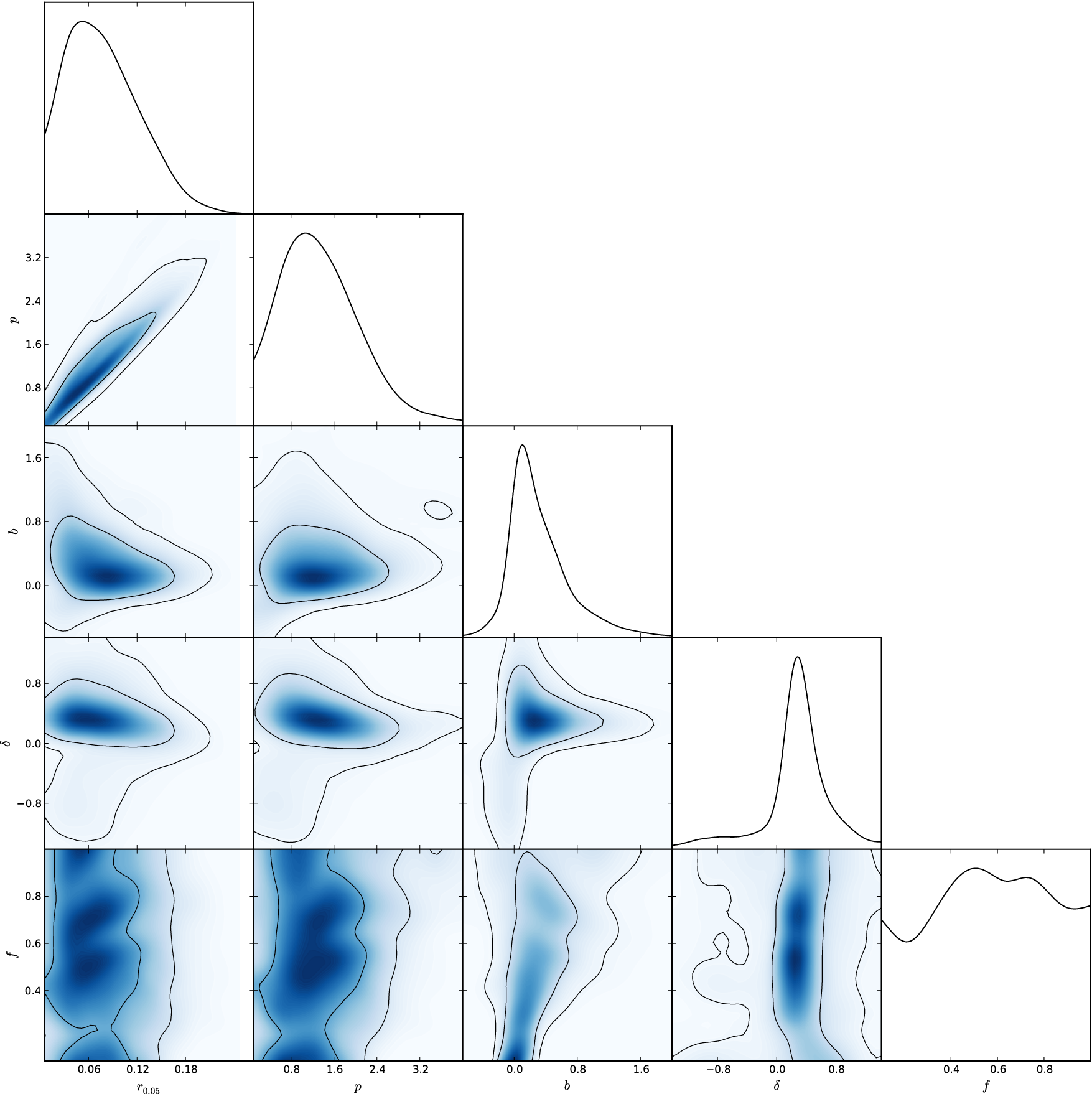
After sampling the parameter space with the data and priors discussed in Section III, we display marginal posterior probability distributions in the model parameters in a “triangle plot” in Figure 1. Starting with the one-dimensional posteriors, it is clear that the oscillation amplitude and phase shift have distributions that are well peaked, albeit with significant non-Gaussian tails. By contrast, the axion decay constant is very poorly constrained, with a mild preference for but largely prior-dominated.


Before proceeding, is important to verify that the constraints on the spectral index and running at the pivot scale Mpc-1 are consistent with those obtained from the usual power-law spectrum and constant running models. To this end, analytic expressions for and are derived in Appendix II and given in equations 31 and 33, respectively. Using these formulas we plot the corresponding derived posteriors in Figures 2(a) and 2(b). The probability is peaked around , entirely consistent with the base Planck model; likewise, the allowed running lies in the approximate range , consistent with the usual constant running model. In Figure 2(c) we plot a posterior in the number of e-foldings (calculated from eq. 13), which shows to be entirely dominated by the chosen flat prior in the fiducial range 50-60. Finally, in Figure 2(d) we plot a posterior in the oscillation period (using eq. 17), which is well-peaked in contrast to the constraint on .
Returning to the model parameter constraints, the structure of the posterior distribution can be better understood from the joint 2-dimensional posteriors in Figure 1. In the vs. plot, one sees a mild correlation in and , particularly for . This can be understood in terms of the running of the spectral index: if the period (corresponding to ) is increased, one must also increase the amplitude to keep the running constant (this can also be seen in the formula for in equation 33). The correlation is not very tight, however, because the required running depends on : the greater the tensor contribution at low , the greater the (negative) running must be to adequately suppress a corresponding amount of low- scalar power.
In Figure 1, we can see in the vs. plot the distribution is obviously multi-modal, where outside the maximum probability region there are three separate “wings”. Two of the wings run off to large or small , while the amplitude is very small or even negative. The third wing runs off to high amplitudes . The multi-modal structure is discussed in further detail in appendix III; here we will simply note that in each of these wings, takes on either very small or large values (as expected since and are correlated). If one stays within the high probability region, is somewhat better constrained than the -posterior in Figure 1 would suggest.
IV.2. Best-fit model
Next, to find the best-fit point by minimizing the likelihood requires some care, because the exact number of e-foldings is computationally too expensive to perform during the minimization procedure. We therefore obtain the best-fit point by factoring in a prior in (given by eq. 15), where in this case our prior is chosen to be strongly peaked (a Gaussian with dispersion =0.5) about a particular value . This procedure is performed over a grid of 16 values regularly spaced from 45 to 65. After finding each best-fit point, the exact number of e-foldings is calculated for each; the best-fit point with the highest likelihood value that remains within the range is chosen as the global best-fit point.
The resulting best-fit parameter values are given in the first row of Table 1. Errors are given for the inflation parameters , , and , determined by the 16% and 84% percentiles of the posterior probability distribution in each parameter.
In Figure 3 we plot the CMB angular power spectrum over the multipole range for the best-fit axion monodromy model (dark line) compared to the base Planck model (red line; defined as the CDM model with a power-law spectrum, i.e. zero running). Note that for , the two models are indistinguishable, while at lower multipoles the axion monodromy power is suppressed by up to 20% compared to the base Planck model. This suppression is a consequence of the running spectral index coming from the sinusoidal term in the potential (eq. 3).
| Best-fit | 0.53 | 2.209 | 67.9 | 0.307 | 0.048 | 0.093 | 58.5 | -0.014 | 0.959 | 0.979 | ||||
|---|---|---|---|---|---|---|---|---|---|---|---|---|---|---|
| 0.13 | 2.37 | 0.41 | 0.20 | 0.58 | 2.216 | 68.2 | 0.304 | 0.048 | 0.094 | 59.9 | -0.020 | 0.960 | 0.970 | |
| 0.19 | 3.08 | 0.31 | 0.12 | 0.54 | 2.210 | 68.3 | 0.303 | 0.048 | 0.093 | 51.9 | -0.025 | 0.960 | 0.961 |
IV.3. Constraints on the tensor-to-scalar ratio and potential parameter
Marginal posteriors in and are shown in Figure 1. Strikingly, the BICEP2 result lies just outside the 99% confidence region, while the highest probability -value is , similar to the best-fit value (Table 1). Likewise, lies outside the 95% confidence region.
From the e-folding constraint given by equation 15 it is apparent that the exponent and the tensor-to-scalar ratio should be strongly correlated, provided the amplitude does not get too large. The joint posterior in and shown in Figure 1 shows that this is indeed the case; a high -value is correlated with a large exponent . The width of the posterior around this correlation is determined by the allowed number of e-foldings, and also the range of -values.
Since the axion decay constant is poorly constrained, it is important to check whether these results are sensitive to the chosen prior on . From the vs. and vs. plot in Figure 1, one can anticipate that the inferred probability of and are weakly dependent on , since essentially no correlation with is seen for either parameter. To verify this, in Figure 4 we plot posterior distributions in for four different assumed priors in : a flat prior in the fiducial range (solid line), a flat prior in the ranges (dashed line) and (dot-dashed line), and finally a log prior in over the fiducial range. As can be seen in the figure, the inferred probability in (and likewise ) is quite robust to changes in the assumed prior. Since the other model parameters (,) are fairly well-constrained, our result for is thus quite insensitive to the priors in the axion model parameters.

Why does the data prefer a small (but nonzero) value? Generally, higher means a larger tensor contribution to anisotropies at low . This exacerbates the deficit in power at low , and thus requires a higher negative running to make up for it. However, the likelihood at high shows no strong preference for negative running (Planck Collaboration et al. 1), and the fit worsens at high as the running increases. Thus, the fit generally worsens as is increased toward large values. This is not the whole story however, because is significantly more constrained in the axion monodromy model compared to the usual constant running model, for which at the 95% confidence level (Planck Collaboration et al. 1). This can be seen in Figure 5, where we plot a joint posterior in vs. for the constant running model (red) and the axion monodromy model (blue). While both models prefer a similar , is more constrained in axion monodromy: the point , lies outside the 95% CL contour for axion monodromy, while it is well within the same contour for the constant running model.
Additionally, note from Figure 5 that prefers to be zero in the constant running model, whereas the axion monodromy model has its peak probability near the best-fit . The reason why axion monodromy does not prefer is simple: one can see from equations 31 and 33 that and are dependent on , whereas in the constant running model, these parameters can be chosen independently of . The best-fit constant running model has a zero tensor contribution () and running . This shows that having a nonzero tensor contribution cannot be entirely made up for by negative running—even if running is allowed, the likelihood itself still prefers . In the axion monodromy model however, this solution is impossible, since the running is proportional to according to equation 32. Thus, would necessarily imply negligible running, and likewise the spectral index would be a poor fit. Instead, the best-fit axion monodromy model settles for an -value () which is high enough to give the necessary running and spectral index, but low enough that the tensor contribution doesn’t spoil the fit too much. This compromise necessarily results in a slightly worse fit at low compared to the constant running model.
We still need to understand why axion monodromy is more restrictive at the large end compared to constant running. To investigate this, Table 2 shows the change in for four models compared to the base Planck model with zero running (). The four models are: the best-fit axion monodromy model (for which ), the best-fit constant running model (for which ), and the same two best-fit models when is fixed to 0.19 rather than varied. Note that while the total is decreased by a similar amount in both best-fit models, is increased in the models, with the axion monodromy giving the worst fit. To understand why this is the case, we must break this down into the various likelihoods representing different multipole ranges.
Starting with the high- likelihoods, note that while the fit to the CAMspec likelihood (comprising the majority of multipoles in the Planck data) is barely affected for the general best-fit models, the fit is dramatically worsened in the models for which . This is a consequence of the aforementioned high running required to fit the low- likelihood well for large . The same is true (though not as dramatically) for the ACT/SPT likelihoods. For the Commander likelihood (low ), on the other hand, all models show an improved fit, but the constant running model gives a significantly better fit; this disparity is greater for the models. In the following section we investigate the nature of this disparity more closely and why it worsens with large .

IV.4. Comparison to constant running model at low multipoles
In Figure 6 we plot the best-fit angular power spectrum for for the base Planck model with zero running (red solid line), axion monodromy (blue dashed line), and constant running (magenta dotted line) models. The black error bars give the errors in each individual multipole. Note that while both models achieve similar reduction in power at very low , the axion monodromy model achieves very little reduction in power for . The deficit in power in the data (points with error bars) is most noticeable over the range , and in this range the constant running model is a significantly better fit.
Why does the constant running model fit the low- likelihood better? There are a few reasons. As discussed in the previous section, axion monodromy does not have the freedom to choose and , independently. In particular, is disfavored because it produces a negligibly small running and incorrect spectral index. Unfortunately however, a nonzero slightly worsens the fit at low by including a tensor contribution.

Even if is fixed to the same value in both models, however, the constant running model achieves a better fit at low . In Figure 7 we plot the primordial scalar power spectrum for axion monodromy models (solid lines) and constant running models (dashed lines), with fixed to 0.07 (dark lines) and 0.19 (red lines) in each case. For either -value, we find that the constant running model achieves greater suppression of power at low (and hence, low ). For the case we need a much greater suppression compared to to make up for the additional tensor power. However, it is evident that the axion monodromy model achieves much less suppression at low compared to the corresponding constant running model. This occurs because the model has a relatively high exponent , as required by the e-folding constraint (eq. 15). As a result, the relatively large monomial term “softens” the magnitude of the running at low . The higher the (and hence, ), the more the running is mitigated at low . This is the principle reason why axion monodromy provides a worse fit compared to constant running when is large.
Even for relatively small amplitudes, as is increased to ever higher values, must also be high (eq. 15). However, sufficiently high solutions lead to a very large or infinite number of e-foldings due to the appearance of a local minimum in the potential from the oscillation (unless the amplitude is very close to zero), as discussed in Section III. This effect excludes nearly all regions of parameter space where , and a large fraction of parameter space where . Thus, the direct effect of the oscillations on the total number of e-foldings restricts the allowed parameter space for large even further.

| Best-fit model | Best-fit constant | Best-fit () | Best-fit constant () | |
|---|---|---|---|---|
| Lowlike (WMAP Pol.) | -0.5 | 0.1 | -1.1 | -1.0 |
| Lensing | 0.8 | 0.9 | 1.0 | 1.2 |
| Commander () | -1.8 | -2.5 | -0.6 | -1.7 |
| CAMspec () | 0.2 | 0.1 | 1.5 | 2.2 |
| ACT/SPT () | -0.5 | -0.2 | 0.2 | -0.1 |
| Total | -1.7 | -1.6 | 1.0 | 0.6 |
IV.5. Comparison to constant running model at high multipoles
As Table 2 shows, axion monodromy actually improves the fit for the ACT/SPT likelihood (high ) compared to the constant running model. We can understand why this is the case from the analytic expression for at the pivot scale (derived in appendix II). The spectral index has two contributions,
| (19) |
where is the contribution from the monomial term in the potential (i.e. the unmodulated spectral index), while is the contribution from the sinusoidal term. By comparing to equation 31 and substituting the approximate e-folding constraint (equation 16), we find that
| (20) | |||||
| (21) |
while for the oscillating term we have
| (22) |
Generally, the first term in equation 22 dominates over the second term provided that the phase shift is not very small or negative, since and are of a similar order. Given that the data prefers a positive , we may therefore expect , and therefore should be at least slightly higher than .
In Figure 2 we plot derived posteriors in and using equations 19, 20, and 22. The constraint in () is quite similar to that obtained in the base Planck model (Planck Collaboration et al. 1), which is expected since it is well constrained by the data. By contrast, the best-fit value for is , which is strikingly high. This follows from equation 21: since the number of e-foldings is restricted to the approximate range 50-60, the lower the -value (and the corresponding -value), the higher must be. Since the best-fit model has , this relatively low accounts for why is so high.

The question remains, why does the data at high prefer such a high ? According to Table 1, the best-fit axion monodromy model shows the greatest improvement in for the ACT/SPT likelihood. We have seen that at high multipoles, the data shows no strong preference for a running spectral index, with preferred even at higher . This is also largely true when the high- data from ACT/SPT is factored in, although it should be noted that ACT and SPT are in tension here; SPT prefers negative running while ACT does not (Di Valentino et al. 54). Thus, while negative running improves the fit at low , it worsens the fit at the high- end unless the running is relatively small. In the best-fit axion monodromy model however, the running diminishes in magnitude as one proceeds to smaller scales (higher ), and hence the spectral index is slightly higher at high . This is why the relatively high value of is preferred, since it allows a smaller running at high .
A similar conclusion regarding a high was reached by [57], in which their best-fit solution has for the case where they incorporate the BICEP2 constraint . However, in their work the full inflation model is not used; the spectral index is chosen completely independently of , and no e-folding constraint is applied. Equation 21 shows that for , cannot be larger than 0.975, and this upper limit is only possible in the limit . From this it can be concluded that while the high- data prefers a high , this is forbidden by the e-folding constraint unless is relatively small. Indeed, the axion monodromy model in Table 1 has and the fit is actually slightly worsened at the high- end.
IV.6. Can the number of e-foldings be amended to allow a higher tensor-to-scalar ratio?
While the e-folding constraint disfavors high -values, one might question whether our model might be amended so that the number of e-foldings satisfies the constraints even for high . In particular, our model assumes that the oscillation amplitude of the potential remains constant all the way to the end of inflation. For this reason, solutions with sufficiently large (and hence ) tend to dramatically inflate the number of e-foldings near the end of inflation, excluding these solutions. However, if the oscillation amplitude were to diminish before the end of inflation, these high- solutions could in principle still satisfy the e-folding constraint.
Furthermore, from the point of view of the underlying microphysics in the axion monodromy model, there is no necessary reason to expect the modulation parameters to remain constant during inflation. On the contrary, these parameters are determined by the values of dynamical moduli fields (e.g. related to the size and shape of the compactified extra-dimensional manifold) which might well evolve with time as inflation progresses. Of course, if the oscillation amplitude were to increase with time, the resulting constraint on would be even stricter. However it is reasonable to consider the case where the oscillation amplitude dies out well before the end of inflation. To consider this, we note that the approximate e-folding parameter (eq. 15) gives the number of e-foldings without the direct contribution of the sinusoidal oscillation; further, by far the largest contribution of the oscillation to the number of e-foldings occurs at scales smaller than that probed by the CMB. This is particularly the case for solutions with high (and hence, high ) values. Therefore, we can use as a conservative estimate of the number of e-foldings in the case where the oscillations die out at scales smaller than that of the CMB.
With this in mind, we apply a flat prior in the number of e-foldings to approximate the case where the amplitude dies out at smaller scales. The resulting constraint on is shown in Figure 8, plotted next to the fiducial result which uses a flat prior in . As can be seen, there is greater probability for large , but even in this case is disfavored at the 95% CL, for the same reason outlined in the previous section: the large amplitude (and low ) required to achieve enough suppression of power at low is forbidden by the e-folding constraint (eq. 15).
In spite of the above difficulties, certainly there are ways to decrease the number of e-foldings to allow for higher . For example, if the exponent switches to a lower value at small scales, inflation would end more quickly and the number of e-foldings would be decreased. From the standpoint of single-field inflation this seems highly unnatural, although such a transition might naturally occur if multiple fields contribute to the effective inflaton potential (for an example of this scenario see Kobayashi et al. 58). From the Occam’s razor point of view however, it seems more likely that the tensor-to-scalar ratio is simply smaller than the BICEP2 result suggests, particularly given the concerns about contamination by dust polarization.

V. Can axion monodromy alleviate the small-scale problems of CDM?
V.1. Implications for dwarf galaxy formation
We have shown that oscillation in the power spectrum can allow for a significant tensor-to-scalar-ratio, alleviating the tension with the standard CDM + power-law spectrum model at very large scales, while still satisfying the e-folding requirement. However, there are also apparent departures from CDM for small-scale structure which can be mitigated by the same mechanism. First, there is the “missing satellites” problem, which refers to the fact that cosmological dissipationless N-body simulations predict a much larger number of dwarf satellite galaxies around the Milky Way than are actually observed (Klypin et al. 59).
The second problem is that in the centers of baryon-poor galaxies the measured dark matter density is systematically lower than predicted by dark matter-only CDM simulations. In many cases, such as in low surface brightness galaxies and field dwarfs with rotation (Kuzio de Naray et al. 60; Simon et al. 61; Adams et al. 62; Gentile et al. 63; Salucci et al. 64; Oh et al. 65), this lower density is due to the presence of a constant dark matter density core (the so-called “core-cusp” problem). The problem seems to extend to the lowest masses, and recent work with dwarfs in the Local Group (Boylan-Kolchin et al. 66; Tollerud et al. 67; Kirby et al. 68) and further away (Ferrero et al. 69) show that they are also systematically under-dense compared to simple expectations from CDM, the so-called “too big to fail” problem (Boylan-Kolchin et al. 70).
It is possible that the simple CDM expectations are incorrect and feedback from supernovae (Governato et al. 71), reionization (Bullock et al. 72), and other effects of star formation (Zolotov et al. 73) all change these expectations dramatically. There is no consensus regarding either of these two problems. Reionization will prevent small satellites from being bright enough to be observed but it is unclear whether this by itself explains the luminosity distribution of the known satellites. There are CDM-based solutions for the second problem but none that alleviate the problem for all the different types of galaxies.

Here we ask whether the reduced power on small scales alleviates some of these issues. If the matter power spectrum is suppressed at the scales Mpc-1, then this would change the formation of dwarf galaxies. Halos would collapse at lower redshift, resulting in lower central dark matter densities. This reduced power may also change the way baryonic feedback operates in low-luminosity systems. This reduction in power has been considered in light of the BICEP2 result: if one allows a constant negative running in the power spectrum to allow for the high tensor-to-scalar ratio reported by BICEP2, [74] found using N-body simulations that the too-big-to-fail problem is significantly alleviated, although not eliminated entirely (it should be noted that baryonic affects are not included in this work). The reduction in power at dwarf scales in this “BICEP2 cosmology” (Abazajian et al. 75) is approximately 40% compared to vanilla CDM. However, as mentioned before, a constant running violates the e-folding constraint. Since the model considered in this work achieves significant running with the requisite amount of e-foldings, we consider here the suppression of power at small scales from our model. Again, we do not assume the BICEP2 result, but rather consider three different -values 0.07, 0.13, and 0.19.
In Figure 9 we plot the relative power obtained by dividing the matter power spectrum in our model by the best-fit Planck power spectrum with zero running. In this plot we use the fitting functions of [76] for the transfer function. For each -value considered, we find the best-fit solution using the same method outlined in Section IV, except with fixed to the given value. We plot the best-fit cases where lies in the fiducial range . Note that for each case, the difference in power compared to the base Planck model comes not only from the primordial power spectrum parameters, but also because of differences in the transfer function which is sensitive to cosmological parameters, particularly and . For we found that most of our solutions had and thus in many cases, a local minimum formed in the potential rendering the number of e-foldings infinite. We did find one solution in the desired range, which is shown in the figure.
At dwarf scales ( Mpc-1), we find an 22% reduction in power for , 28% reduction for , and 33% reduction for . This is not as drastic a reduction as in the BICEP2 cosmology ( 40%), and recall in addition that is disfavored by the Planck data (Figure 4). Nevertheless, a reduction in power of 20-30% is entirely consistent with the data and e-folding constraint, and may be expected to alleviate the too-big-to-fail problem, particularly when considered in combination with baryonic feedback effects. One can also see from Figure 9 that even greater suppression occurs at smaller scales, and this has a bearing on the missing satellites problem. In addition, the corresponding suppression of substructure would substantially reduce the expected dark matter annihilation signal (Garrison-Kimmel et al. 74).

V.2. Comparison to power spectrum constraints from Lyman- forest data
Aside from dwarf galaxies, another approach to detect oscillations in the power spectrum is to observe at high redshift where the matter power spectrum is close to linear at small scales. The Lyman- forest observed in quasar spectra can reveal structure down to 100 kpc scales in the approximate redshift range to , which is in the quasi-linear regime. Past studies have found constraints on the running of the spectral index, though not with the accuracy required for a positive detection of running of order (Seljak et al. 79; Viel et al. 80). However, more recent quasar observations by the Baryon Oscillation Spectroscopic Survey (BOSS) collaboration (Dawson et al. 81; Palanque-Delabrouille et al. 78) have dramatically enlarged the available dataset of quasars with measured Ly forest power spectra. In Figure 10 we plot inferred probability contours in the amplitude and slope of the linear matter power spectrum at and km/s (corresponding to roughly 1 Mpc scales). The grey contours are from [77], while the green contours are from the more recent data from [82]. The red and blue contours are from derived posterior probability distributions for axion monodromy and the base Planck model respectively. From this figure it is evident that while the older data cannot distinguish between the two models, the new BOSS data favors axion monodromy: the base Planck model prediction for is more than 2-sigma apart from that of [82], while the axion monodromy prediction is consistent to within 1-sigma. More generally, this comparison indicates that a negative running in the power spectrum may now be favored by recent Ly forest data, at the level required to accommodate a substantial tensor-to-scalar ratio.
There are a number of other approaches to probing the small-scale power spectrum besides Lyman- forest data. Down the road, 21-cm observations are a promising approach to constraining the power spectrum at even smaller scales (Shimabukuro et al. 83) since, unlike the Lyman- forest, much higher redshifts can be probed where the data is not as limited at large by thermal broadening. In the meantime, resolving the discrepancy between SPT and ACT on whether negative running is preferred in the CMB at high will be an important step. Within the coming decade, advanced redshift surveys such as WFIRST (Spergel et al. 84) and LSST may offer the best window onto the power spectrum at scales smaller than CMB (Meerburg 57), with the caveat that galaxy bias must be properly taken into account. In any event, a non-trivial primordial power spectrum remains an intriguing possibility for alleviating small-scale problems. This will be true particularly if alternate forms of dark matter (WDM, self-interacting) are ruled out as solutions to the too-big-to-fail and/or missing satellites problems.
VI. Conclusions
In this paper we have investigated whether inflation models can allow for a large gravitational wave background while remaining consistent with the CMB power spectrum at horizon scales (low ). We have shown that axion monodromy inflation accomplishes this naturally through Planck-scale corrections, producing a gentle oscillation in the inflaton potential (eq. 2). This generates a running spectral index in the power spectrum while still achieving enough e-foldings to solve the horizon problem, in stark contrast to the usual constant running model. We have fit our model to a combination of Planck, ACT, SPT, and WMAP low- polarization CMB data together with a prior on the number of e-foldings. The best-fit model parameters are given in Table 1, while inferred probability distributions in the inflation model parameters are shown in Figure 1.
We find a best-fit tensor-to-scalar ratio and thus the predicted imprint of gravitational waves on the CMB is within reach of B-mode polarization experiments. It is possible that these primordial B-modes have already been observed by the BICEP2 experiment; however if one assumes neglible foreground contamination, the BICEP2 result is disfavored at the 99% confidence level. This is primarily a consequence of the e-folding constraint and the requirement to fit the spectral index at high in addition to the low- power spectrum. Since a running spectral index is the most straightforward way to reconcile the BICEP2 result with Planck, it is significant that attempting to implement running in the underlying inflation theory disfavors such a large , as we have shown here. While it is possible that a dramatic change in the inflaton potential at small scales (high ) can alter the e-folding constraint to allow for a higher , we find it more likely that the tensor-to-scalar ratio is simply smaller than the best-fit BICEP2 result suggests, particularly in light of the uncertainties about foreground contamination by dust polarization in the BICEP2 field.
In addition to the large gravitational wave amplitude, the (best-fit) axion monodromy model makes two corresponding predictions: first, despite the additional tensor power on horizon scales, the overall power at low multipoles is reduced as a consequence of the running spectral index, providing a better fit to the CMB power spectrum at large scales. The second prediction is that the matter power spectrum is suppressed at the scale of dwarf galaxies, and thus axion monodromy can alleviate some of the small-scale problems of CDM—in particular, the too-big-to-fail and missing satellites problems. We find that our best-fit models reduce the power at scales relevant to dwarf galaxy formation ( Mpc-1) by as much as 35% depending on the assumed -value, with the greatest reduction achieved at large . However, 20-30% suppression is more likely, which will alleviate the too-big-to-fail problem and may solve it entirely when combined with baryonic feedback effects, as discussed in [74]. Additionally, we find that axion monodromy is preferred by recent Ly forest data over the base Planck model without running (Figure 10).
If axion monodromy (or a similar oscillating large-field model) accounts for the reduced power at large and small scales, then the tensor-to-scalar ratio is likely to lie in the range (68% CL) and hence the imprint of gravitational waves on the CMB will be observable by B-mode experiments in the future (Abazajian et al. 85). With this comes the tantalizing prospect of constraining physics at the Planck scale through sky surveys, as we have demonstrated here. Thus, future CMB experiments, in combination with probes of the power spectrum at small scales, may settle the issue of whether Planck-scale physics manifest in inflation can reconcile the standard CDM cosmology with data at all observable scales of the Universe.
Acknowledgements
QM would like to thank James Bullock, Shahab Joudaki, Jose Ceja and Shea Garrison-Kimmel for their encouragement and feedback at the beginning stages of this project.
We gratefully acknowledge a grant of computer time from XSEDE allocation TG-AST130007. MK was supported in part by NSF grant PHY-1214648.
This research was also supported, in part, by a grant of computer time from the City University of New York High Performance Computing Center under NSF Grants CNS-0855217, CNS-0958379 and ACI-1126113.
References
- [1] Planck Collaboration, P. A. R. Ade, N. Aghanim, C. Armitage-Caplan, M. Arnaud, M. Ashdown, F. Atrio-Barandela, J. Aumont, C. Baccigalupi, A. J. Banday, et al., ArXiv e-prints (2013a), arXiv:1303.5076 [astro-ph.CO] .
- [2] Planck Collaboration, P. A. R. Ade, N. Aghanim, C. Armitage-Caplan, M. Arnaud, M. Ashdown, F. Atrio-Barandela, J. Aumont, C. Baccigalupi, A. J. Banday, and et al., ArXiv e-prints (2013b), arXiv:1303.5083 [astro-ph.CO] .
- [3] D. N. Spergel, L. Verde, H. V. Peiris, E. Komatsu, M. R. Nolta, C. L. Bennett, M. Halpern, G. Hinshaw, N. Jarosik, A. Kogut, M. Limon, S. S. Meyer, L. Page, G. S. Tucker, J. L. Weiland, E. Wollack, and E. L. Wright, ApJS 148, 175 (2003), astro-ph/0302209 .
- [4] G. Hinshaw, D. N. Spergel, L. Verde, R. S. Hill, S. S. Meyer, C. Barnes, C. L. Bennett, M. Halpern, N. Jarosik, A. Kogut, E. Komatsu, M. Limon, L. Page, G. S. Tucker, J. L. Weiland, E. Wollack, and E. L. Wright, ApJS 148, 135 (2003), astro-ph/0302217 .
- [5] B. Feng, M. Li, R.-J. Zhang, and X. Zhang, Phys. Rev. D 68, 103511 (2003), astro-ph/0302479 .
- [6] M. Bastero-Gil, K. Freese, and L. Mersini-Houghton, Phys. Rev. D 68, 123514 (2003), hep-ph/0306289 .
- [7] D. J. Chung, G. Shiu, and M. Trodden, Phys. Rev. D 68, 063501 (2003), astro-ph/0305193 .
- [8] M. Kawasaki, M. Yamaguchi, and J. Yokoyama, Phys. Rev. D 68, 023508 (2003), hep-ph/0304161 .
- [9] P. Hunt and S. Sarkar, Phys. Rev. D 76, 123504 (2007), arXiv:0706.2443 .
- [10] H. V. Peiris, E. Komatsu, L. Verde, D. N. Spergel, C. L. Bennett, M. Halpern, G. Hinshaw, N. Jarosik, A. Kogut, M. Limon, S. S. Meyer, L. Page, G. S. Tucker, E. Wollack, and E. L. Wright, ApJS 148, 213 (2003), astro-ph/0302225 .
- [11] C. R. Contaldi, M. Peloso, L. Kofman, and A. Linde, J. Cosmology Astropart. Phys 7, 002 (2003), astro-ph/0303636 .
- [12] M. J. Mortonson, C. Dvorkin, H. V. Peiris, and W. Hu, Phys. Rev. D 79, 103519 (2009), arXiv:0903.4920 [astro-ph.CO] .
- [13] D. K. Hazra, A. Shafieloo, G. F. Smoot, and A. A. Starobinsky, J. Cosmology Astropart. Phys 8, 048 (2014), arXiv:1405.2012 .
- [14] L. Lello and D. Boyanovsky, J. Cosmology Astropart. Phys 5, 029 (2014), arXiv:1312.4251 .
- [15] Y.-S. Piao, B. Feng, and X. Zhang, Phys. Rev. D 69, 103520 (2004), hep-th/0310206 .
- [16] J. White, Y.-l. Zhang, and M. Sasaki, Phys. Rev. D 90, 083517 (2014), arXiv:1407.5816 .
- [17] A. Ashoorioon, K. Dimopoulos, M. M. Sheikh-Jabbari, and G. Shiu, Physics Letters B 737, 98 (2014), arXiv:1403.6099 [hep-th] .
- [18] C. Dvorkin, M. Wyman, D. H. Rudd, and W. Hu, ArXiv e-prints (2014), arXiv:1403.8049 .
- [19] L. A. Anchordoqui, ArXiv e-prints (2014), arXiv:1407.8105 .
- [20] K. M. Smith, C. Dvorkin, L. Boyle, N. Turok, M. Halpern, G. Hinshaw, and B. Gold, Physical Review Letters 113, 031301 (2014), arXiv:1404.0373 .
- [21] P. A. R. Ade, R. W. Aikin, D. Barkats, et al., Physical Review Letters 112, 241101 (2014), arXiv:1403.3985 .
- [22] R. Flauger, J. C. Hill, and D. N. Spergel, J. Cosmology Astropart. Phys 8, 039 (2014), arXiv:1405.7351 .
- [23] M. J. Mortonson and U. Seljak, ArXiv e-prints (2014), arXiv:1405.5857 .
- [24] Planck Collaboration, R. Adam, P. A. R. Ade, N. Aghanim, M. Arnaud, J. Aumont, C. Baccigalupi, A. J. Banday, R. B. Barreiro, J. G. Bartlett, and et al., ArXiv e-prints (2014), arXiv:1409.5738 .
- [25] D. H. Lyth, Physical Review Letters 78, 1861 (1997), hep-ph/9606387 .
- [26] Planck Collaboration, P. A. R. Ade, N. Aghanim, C. Armitage-Caplan, M. Arnaud, M. Ashdown, F. Atrio-Barandela, J. Aumont, C. Baccigalupi, A. J. Banday, and et al., ArXiv e-prints (2013c), arXiv:1303.5082 [astro-ph.CO] .
- [27] R. Easther and H. V. Peiris, J. Cosmology Astropart. Phys 9, 010 (2006), astro-ph/0604214 .
- [28] G. Ballesteros, J. A. Casas, J. R. Espinosa, R. Ruiz de Austri, and R. Trotta, J. Cosmology Astropart. Phys 3, 018 (2008), arXiv:0711.3436 [hep-ph] .
- [29] G. Ballesteros and J. A. Casas, ArXiv e-prints (2014), arXiv:1406.3342 .
- [30] D. K. Hazra, A. Shafieloo, G. F. Smoot, and A. A. Starobinsky, Phys.Rev.Lett. 113, 071301 (2014), arXiv:1404.0360 [astro-ph.CO] .
- [31] A. Ashoorioon and A. Krause, ArXiv High Energy Physics - Theory e-prints (2006), hep-th/0607001 .
- [32] E. Silverstein and A. Westphal, Phys. Rev. D 78, 106003 (2008), arXiv:0803.3085 [hep-th] .
- [33] N. Kaloper and L. Sorbo, Physical Review Letters 102, 121301 (2009), arXiv:0811.1989 [hep-th] .
- [34] L. McAllister, E. Silverstein, and A. Westphal, Phys. Rev. D 82, 046003 (2010), arXiv:0808.0706 [hep-th] .
- [35] N. Kaloper, A. Lawrence, and L. Sorbo, J. Cosmology Astropart. Phys 3, 023 (2011), arXiv:1101.0026 [hep-th] .
- [36] T. Kobayashi and F. Takahashi, J. Cosmology Astropart. Phys 1, 026 (2011), arXiv:1011.3988 [astro-ph.CO] .
- [37] K. Freese, J. A. Frieman, and A. V. Olinto, Physical Review Letters 65, 3233 (1990).
- [38] S. Dimopoulos, S. Kachru, J. McGreevy, and J. G. Wacker, J. Cosmology Astropart. Phys 8, 003 (2008), hep-th/0507205 .
- [39] Y. Wan, S. Li, M. Li, T. Qiu, Y. Cai, and X. Zhang, Phys. Rev. D 90, 023537 (2014), arXiv:1405.2784 .
- [40] I. P. Neupane, Phys. Rev. D 90, 123502 (2014), arXiv:1409.8647 .
- [41] R. Flauger, L. McAllister, E. Pajer, A. Westphal, and G. Xu, J. Cosmology Astropart. Phys 6, 009 (2010), arXiv:0907.2916 [hep-th] .
- [42] M. Aich, D. K. Hazra, L. Sriramkumar, and T. Souradeep, Phys.Rev. D87, 083526 (2013), arXiv:1106.2798 [astro-ph.CO] .
- [43] L. McAllister, E. Silverstein, A. Westphal, and T. Wrase, ArXiv e-prints (2014), arXiv:1405.3652 [hep-th] .
- [44] V. F. Mukhanov, H. A. Feldman, and R. H. Brandenberger, Phys. Rep. 215, 203 (1992).
- [45] D. Baumann, ArXiv e-prints (2009), arXiv:0907.5424 [hep-th] .
- [46] Note that the scale of the potential will not enter into our equations directly, since we only encounter the combination . Nevertheless, is not an independent parameter but is rather determined by the normalization of , with the result in the slow roll approximation.
- [47] A. Lewis and S. Bridle, Phys. Rev. D 66, 103511 (2002), astro-ph/0205436 .
- [48] A. Lewis, Phys. Rev. D 87, 103529 (2013), arXiv:1304.4473 [astro-ph.CO] .
- [49] Planck collaboration, P. A. R. Ade, N. Aghanim, C. Armitage-Caplan, M. Arnaud, M. Ashdown, F. Atrio-Barandela, J. Aumont, C. Baccigalupi, A. J. Banday, and et al., ArXiv e-prints (2013), arXiv:1303.5075 [astro-ph.CO] .
- [50] G. Hinshaw, D. Larson, E. Komatsu, D. N. Spergel, C. L. Bennett, J. Dunkley, M. R. Nolta, M. Halpern, R. S. Hill, N. Odegard, L. Page, K. M. Smith, J. L. Weiland, B. Gold, N. Jarosik, A. Kogut, M. Limon, S. S. Meyer, G. S. Tucker, E. Wollack, and E. L. Wright, ApJS 208, 19 (2013), arXiv:1212.5226 [astro-ph.CO] .
- [51] K. T. Story, C. L. Reichardt, Z. Hou, et al., ApJ 779, 86 (2013), arXiv:1210.7231 [astro-ph.CO] .
- [52] J. L. Sievers, R. A. Hlozek, M. R. Nolta, et al., J. Cosmology Astropart. Phys 10, 060 (2013), arXiv:1301.0824 [astro-ph.CO] .
- [53] To be precise, a very large number of e-foldings would occur until the field tunnels out of the local minimum via bubble nucleation. Given that relatively few e-foldings would follow this before inflation ends, this scenario would produce an open universe with a very sub-critical energy density, in gross violation of cosmological constraints (see for example [86]).
- [54] E. Di Valentino, S. Galli, M. Lattanzi, A. Melchiorri, P. Natoli, L. Pagano, and N. Said, Phys. Rev. D 88, 023501 (2013), arXiv:1301.7343 [astro-ph.CO] .
- [55] J. E. Kim, H. P. Nilles, and M. Peloso, J. Cosmology Astropart. Phys 1, 005 (2005), hep-ph/0409138 .
- [56] R. Kappl, S. Krippendorf, and H. P. Nilles, Physics Letters B 737, 124 (2014), arXiv:1404.7127 [hep-th] .
- [57] P. D. Meerburg, ArXiv e-prints (2014), arXiv:1406.3243 .
- [58] T. Kobayashi, O. Seto, and Y. Yamaguchi, ArXiv e-prints (2014), arXiv:1404.5518 [hep-ph] .
- [59] A. Klypin, A. V. Kravtsov, O. Valenzuela, and F. Prada, ApJ 522, 82 (1999), astro-ph/9901240 .
- [60] R. Kuzio de Naray, S. S. McGaugh, W. J. G. de Blok, and A. Bosma, ApJS 165, 461 (2006), astro-ph/0604576 .
- [61] J. D. Simon, A. D. Bolatto, A. Leroy, L. Blitz, and E. L. Gates, ApJ 621, 757 (2005), astro-ph/0412035 .
- [62] J. J. Adams, J. D. Simon, M. H. Fabricius, R. C. E. van den Bosch, J. C. Barentine, R. Bender, K. Gebhardt, G. J. Hill, J. D. Murphy, R. A. Swaters, J. Thomas, and G. van de Ven, ApJ 789, 63 (2014), arXiv:1405.4854 .
- [63] G. Gentile, P. Salucci, U. Klein, D. Vergani, and P. Kalberla, MNRAS 351, 903 (2004), astro-ph/0403154 .
- [64] P. Salucci, M. I. Wilkinson, M. G. Walker, G. F. Gilmore, E. K. Grebel, A. Koch, C. Frigerio Martins, and R. F. G. Wyse, MNRAS 420, 2034 (2012), arXiv:1111.1165 [astro-ph.CO] .
- [65] S.-H. Oh, W. J. G. de Blok, E. Brinks, F. Walter, and R. C. Kennicutt, Jr., AJ 141, 193 (2011), arXiv:1011.0899 [astro-ph.CO] .
- [66] M. Boylan-Kolchin, J. S. Bullock, and M. Kaplinghat, MNRAS 422, 1203 (2012), arXiv:1111.2048 [astro-ph.CO] .
- [67] E. J. Tollerud, M. Boylan-Kolchin, and J. S. Bullock, MNRAS 440, 3511 (2014), arXiv:1403.6469 .
- [68] E. N. Kirby, J. S. Bullock, M. Boylan-Kolchin, M. Kaplinghat, and J. G. Cohen, MNRAS 439, 1015 (2014), arXiv:1401.1208 .
- [69] I. Ferrero, M. G. Abadi, J. F. Navarro, L. V. Sales, and S. Gurovich, MNRAS 425, 2817 (2012), arXiv:1111.6609 [astro-ph.CO] .
- [70] M. Boylan-Kolchin, J. S. Bullock, and M. Kaplinghat, MNRAS 415, L40 (2011), arXiv:1103.0007 [astro-ph.CO] .
- [71] F. Governato, A. Zolotov, A. Pontzen, C. Christensen, S. H. Oh, A. M. Brooks, T. Quinn, S. Shen, and J. Wadsley, MNRAS 422, 1231 (2012), arXiv:1202.0554 [astro-ph.CO] .
- [72] J. S. Bullock, A. V. Kravtsov, and D. H. Weinberg, ApJ 539, 517 (2000), astro-ph/0002214 .
- [73] A. Zolotov, A. M. Brooks, B. Willman, F. Governato, A. Pontzen, C. Christensen, A. Dekel, T. Quinn, S. Shen, and J. Wadsley, ApJ 761, 71 (2012), arXiv:1207.0007 [astro-ph.CO] .
- [74] S. Garrison-Kimmel, S. Horiuchi, K. N. Abazajian, J. S. Bullock, and M. Kaplinghat, MNRAS 444, 961 (2014), arXiv:1405.3985 .
- [75] K. N. Abazajian, G. Aslanyan, R. Easther, and L. C. Price, J. Cosmology Astropart. Phys 8, 053 (2014), arXiv:1403.5922 .
- [76] D. J. Eisenstein and W. Hu, ApJ 496, 605 (1998), astro-ph/9709112 .
- [77] P. McDonald, U. Seljak, R. Cen, D. Shih, D. H. Weinberg, S. Burles, D. P. Schneider, D. J. Schlegel, N. A. Bahcall, J. W. Briggs, J. Brinkmann, M. Fukugita, Ž. Ivezić, S. Kent, and D. E. Vanden Berk, ApJ 635, 761 (2005), astro-ph/0407377 .
- [78] N. Palanque-Delabrouille, C. Yèche, A. Borde, J.-M. Le Goff, G. Rossi, M. Viel, É. Aubourg, S. Bailey, J. Bautista, M. Blomqvist, A. Bolton, J. S. Bolton, N. G. Busca, B. Carithers, R. A. C. Croft, K. S. Dawson, T. Delubac, A. Font-Ribera, S. Ho, D. Kirkby, K.-G. Lee, D. Margala, J. Miralda-Escudé, D. Muna, A. D. Myers, P. Noterdaeme, I. Pâris, P. Petitjean, M. M. Pieri, J. Rich, E. Rollinde, N. P. Ross, D. J. Schlegel, D. P. Schneider, A. Slosar, and D. H. Weinberg, A&A 559, A85 (2013), arXiv:1306.5896 [astro-ph.CO] .
- [79] U. Seljak, A. Slosar, and P. McDonald, J. Cosmology Astropart. Phys 10, 014 (2006), astro-ph/0604335 .
- [80] M. Viel, J. Weller, and M. G. Haehnelt, MNRAS 355, L23 (2004), astro-ph/0407294 .
- [81] K. S. Dawson, D. J. Schlegel, C. P. Ahn, S. F. Anderson, and et al., AJ 145, 10 (2013), arXiv:1208.0022 [astro-ph.CO] .
- [82] N. Palanque-Delabrouille, C. Yèche, J. Lesgourgues, G. Rossi, A. Borde, M. Viel, E. Aubourg, D. Kirkby, J.-M. LeGoff, J. Rich, N. Roe, N. P. Ross, D. P. Schneider, and D. Weinberg, ArXiv e-prints (2014), arXiv:1410.7244 .
- [83] H. Shimabukuro, K. Ichiki, S. Inoue, and S. Yokoyama, Phys. Rev. D 90, 083003 (2014), arXiv:1403.1605 .
- [84] D. Spergel, N. Gehrels, J. Breckinridge, et al., ArXiv e-prints (2013), arXiv:1305.5425 [astro-ph.IM] .
- [85] K. N. Abazajian, K. Arnold, J. Austermann, et al., ArXiv e-prints (2013), arXiv:1309.5381 .
- [86] M. Bucher, A. S. Goldhaber, and N. Turok, Phys. Rev. D 52, 3314 (1995), hep-ph/9411206 .
I. Appendix: Is the slow roll approximation valid in our model?
When there are oscillating features in the power spectrum, the slow roll approximation can be violated, particularly for short-period oscillations. Thus, it is important to check that the slow roll approximation we have used here is valid in the parameter range we are interested in. For the slow roll approximation to hold, both the first slow roll parameter and the second slow roll parameter must be small, such that . The former condition is obviously satisfied at CMB scales, as we are many e-foldings before the end of inflation and thus . The second condition is trickier, however, because rapid oscillation can cause to become large. To estimate , we must solve the classical equation of motion for :
| (23) |
Since is small, we have . Let us switch variables to , where can be interpreted as the time in units of the Hubble time when the mode leaves the horizon. We then find
| (24) |
This equation can be solved numerically, using the expression for the (scaled) potential and its derivative from equation 3. Here, since we are interested in an analytic expression for , we will use a method similar to that of [41] and try a solution of the form , where is the unmodulated scalar field, contains the oscillation and the amplitude is assumed to be small (as it must be). For , the slow roll approximation holds very well, as usual, so we can ignore . Substituting this expression in to equation 24 and separating out the zeroth order and first order terms, we find for the zeroth order equation
| (25) |
We will not need to solve this equation exactly for the present discussion, but we note that since we are 50-60 e-foldings from the end of inflation, we have and hence, .
Proceeding to the first-order equation, we switch to using as the independent variable, yielding the equation
| (26) |
where the prime denotes the derivative . To solve this equation we try a linear combination of sines and cosines, and arrive at the solution
| (27) |
where is an unimportant phase factor. We can now estimate the amplitude of the slow roll parameter . Plugging in eqs. 25 and 27, we find
| (28) |
This is well approximated as
| (29) |
where we have made use of equations 11, 12, and 14. Note that if the amplitude is kept fixed, can be made large (and hence, slow roll violated) if is sufficiently small.

For the best-fit solution in Table 1, we have and thus the slow roll description holds. On the other hand, at
the extreme ends of the parameter space we have chosen, can become
large; for example, setting , can give comparable to
1. Fortunately, such regions where slow roll breaks down are excluded by the
data. To show this robustly, in Figure 11 we plot a derived
posterior in using equation 28, with the same priors
and data as discussed in Section III. For all the points sampled,
we have , and hence the slow roll approximation holds
good for all allowed regions of parameter space. This justifies our use of the
slow roll approximation in deriving the power spectra in Section
II.2.
II. Appendix: Expressions for the spectral index and running in the slow-roll approximation
To relate the parameters to observable features, it is useful to have expressions for the spectral index and running at the pivot scale. The most useful expressions we derive will be equations 31 and 33, which are given in terms of the fit parameters in the usual case where , and the running is dominated by the sinusoidal term.
II.1. Spectral index
To derive expressions for the spectral index, we can use the relation in terms of the slow roll parameters, . Using the fact that and , we find using equation 3,
| (30) |
where it is understood that we are evaluating the spectral index at the pivot scale . Substituting equation 10 and keeping terms to first order in , we find (after substituting equation 11),
| (31) |
Note that the oscillation is dominated by the sine term (unless is very small such that ), and thus the amplitude of the spectral index oscillation is . Our constraint in is plotted in Figure 2(a) and is consistent with the result found by applying the base Planck model.
II.2. Running of the spectral index
As discussed in Section IV, the best fit parameters are characterized by a substantial running of the spectral index which is dominated by the sinusoidal term. To first order, the running can be calculated from where is the third potential slow roll parameter. From this we find (at the pivot scale ),
| (32) |
From this formula it is evident that the running oscillates in with the approximate amplitude .
Now we derive the more exact expression for the running using the formula . Expanding this to first order in and up to second order in , we obtain
| (33) |
The last term above is due to the monomial term in the potential, and is clearly of order if ; the middle term is typically of a similar order. For the best fits, we have , in which case the above formula is accurate for up to two significant figures. Our constraint in the running is plotted in Figure 2(b).


III. Appendix: Structure of the posterior distribution
As discussed in Section IV, the posterior distribution has a complicated multi-modal structure, with several non-Gaussian tails running away from the best-fit region. To understand this structure better, in Figure 12 we plot 3-dimensional posteriors with the axes for and shown, color-coded by , , and respectively. Note there are three separate “wings” in the distribution running away from the best-fit region, and in all of these wings the tensor-to-scalar ratio prefers to be small (Figure 12). This is because large must be accommodated by a large negative running, and in Figure 12 one sees that a large negative running only occurs in the best-fit region, whereas it is quite small in the wings. Two of the wings have , which then naturally would imply a small running; however, the other wing has a large amplitude . How can the running be small in this case? The answer can be seen in Figure 12: in most of this region (corresponding to the period) is quite large, and thus the running is again small. Note that in all the wings tends to take on either very small () or very large values (), with intermediate values occurring mostly in the best-fit region. For this reason, if one stays within the best-fit region, the axion decay constant is somewhat better constrained than is suggested by the posterior in Figure 1 although the errors are still large.