Distributed Submodular Maximization
Abstract
Many large-scale machine learning problems–clustering, non-parametric learning, kernel machines, etc.–require selecting a small yet representative subset from a large dataset. Such problems can often be reduced to maximizing a submodular set function subject to various constraints. Classical approaches to submodular optimization require centralized access to the full dataset, which is impractical for truly large-scale problems. In this paper, we consider the problem of submodular function maximization in a distributed fashion. We develop a simple, two-stage protocol GreeDi, that is easily implemented using MapReduce style computations. We theoretically analyze our approach, and show that under certain natural conditions, performance close to the centralized approach can be achieved. We begin with monotone submodular maximization subject to a cardinality constraint, and then extend this approach to obtain approximation guarantees for (not necessarily monotone) submodular maximization subject to more general constraints including matroid or knapsack constraints. In our extensive experiments, we demonstrate the effectiveness of our approach on several applications, including sparse Gaussian process inference and exemplar based clustering on tens of millions of examples using Hadoop.
keywords
distributed computing, submodular functions, approximation algorithms, greedy algorithms, map-reduce1 Introduction
Numerous machine learning tasks require selecting representative subsets of manageable size out of large datasets. Examples range from exemplar based clustering (Dueck and Frey, 2007) to active set selection for non-parametric learning (Rasmussen, 2004), to viral marketing (Kempe et al., 2003), and data subset selection for the purpose of training complex models (Lin and Bilmes, 2011). Many such problems can be reduced to the problem of maximizing a submodular set function subject to cardinality or other feasibility constraints such as matroid, or knapsack constraints (Krause and Gomes, 2010; Krause and Golovin, 2012; Lee et al., 2009a).
Submodular functions exhibit a natural diminishing returns property common in many well known objectives: the marginal benefit of any given element decreases as we select more and more elements. Functions such as entropy or maximum weighted coverage are typical examples of functions with diminishing returns. As a result, submodular function optimization has numerous applications in machine learning and social networks: viral marketing (Kempe et al., 2003; Babaei et al., 2013; Mirzasoleiman et al., 2012), information gathering (Krause and Guestrin, 2011), document summarization (Lin and Bilmes, 2011), and active learning (Golovin and Krause, 2011; Guillory and Bilmes, 2011).
Although maximizing a submodular function is NP-hard in general, a seminal result of Nemhauser et al. (1978) states that a simple greedy algorithm produces solutions competitive with the optimal (intractable) solution (Nemhauser and Wolsey, 1978; Feige, 1998). However, such greedy algorithms or their accelerated variants (Minoux, 1978; Badanidiyuru and Vondrák, 2014; Mirzasoleiman et al., 2015a) do not scale well when the dataset is massive. As data volumes in modern applications increase faster than the ability of individual computers to process them, we need to look at ways to adapt our computations using parallelism.
MapReduce (Dean and Ghemawat, 2008) is arguably one of the most successful programming models for reliable and efficient parallel computing. It works by distributing the data to independent machines: map tasks redistribute the data for appropriate parallel processing and the output then gets sorted and processed in parallel by reduce tasks.
To perform submodular optimization in MapReduce, we need to design suitable parallel algorithms. The greedy algorithms that work well for centralized submodular optimization do not translate easily to parallel environments. The algorithms are inherently sequential in nature, since the marginal gain from adding each element is dependent on the elements picked in previous iterations. This mismatch makes it inefficient to apply classical algorithms directly to parallel setups.
In this paper, we develop a distributed procedure for maximizing submodular functions, that can be easily implemented in MapReduce. Our strategy is to partition the data (e.g., randomly) and process it in parallel. In particular:
- •
We present a simple, parallel protocol, called GreeDi for distributed submodular maximization subject to cardinality constraints. It requires minimal communication, and can be easily implemented in MapReduce style parallel computation models.
- •
We show that under some natural conditions, for large datasets the quality of the obtained solution is provably competitive with the best centralized solution.
- •
We discuss extensions of our approach to obtain approximation algorithms for (not-necessarily monotone) submodular maximization subject to more general types of constraints, including matroid and knapsack constraints.
- •
We implement our approach for exemplar based clustering and active set selection in Hadoop, and show how our approach allows to scale exemplar based clustering and sparse Gaussian process inference to datasets containing tens of millions of points.
- •
We extensively evaluate our algorithm on several machine learning problems, including exemplar based clustering, active set selection and finding cuts in graphs, and show that our approach leads to parallel solutions that are very competitive with those obtained via centralized methods ( in exemplar based clustering, in active set selection, in finding cuts).
This paper is organized as follows. We begin in Section 2 by discussing background and related work. In Section 3, we formalize the distributed submodular maximization problem under cardinality constraints, and introduce example applications as well as naive approaches toward solving the problem. We subsequently present our GreeDi algorithm in Section 4, and prove its approximation guarantees. We then consider maximizing a submodular function subject to more general constraints in Section 5. We also present computational experiments on very large datasets in Section 6, showing that in addition to its provable approximation guarantees, our algorithm provides results close to the centralized greedy algorithm. We conclude in Section 7.
2 Background and Related Work
2.1 Distributed Data Analysis and MapReduce
Due to the rapid increase in dataset sizes, and the relatively slow advances in sequential processing capabilities of modern CPUs, parallel computing paradigms have received much interest. Inhabiting a sweet spot of resiliency, expressivity and programming ease, the MapReduce style computing model (Dean and Ghemawat, 2008) has emerged as prominent foundation for large scale machine learning and data mining algorithms (Chu et al., 2007; Ekanayake et al., 2008). A MapReduce job takes the input data as a set of pairs. Each job consists of three stages: the map stage, the shuffle stage, and the reduce stage. The map stage, partitions the data randomly across a number of machines by associating each element with a key and produce a set of pairs. Then, in the shuffle stage, the value associated with all of the elements with the same key gets merged and send to the same machine. Each reducer then processes the values associated with the same key and outputs a set of new pairs with the same key. The reducers’ output could be input to another MapReduce job and a program in MapReduce paradigm can consist of multiple rounds of map and reduce stages (Karloff et al., 2010).
2.2 Centralized and Streaming Submodular Maximization
The problem of centralized maximization of submodular functions has received much interest, starting with the seminal work of Nemhauser et al. (1978). Recent work has focused on providing approximation guarantees for more complex constraints (Krause and Golovin, 2012, for a more detailed account, see the recent survey by). Golovin et al. (2010) consider an algorithm for online distributed submodular maximization with an application to sensor selection. However, their approach requires stages of communication, which is unrealistic for large in a MapReduce style model. Krause and Gomes (2010) consider the problem of submodular maximization in a streaming model; however, their approach makes strong assumptions about the way the data stream is generated and is not applicable to the general distributed setting. Recently, Badanidiyuru et al. (2014) provide a single pass streaming algorithm for cardinality-constrained submodular maximization with approximation guarantee to the optimum solution that makes no assumptions on the data stream.
There has also been new improvements in the running time of the standard greedy solution for solving SET-COVER (a special case of submodular maximization) when the data is large and disk resident (Cormode et al., 2010). More generally, Badanidiyuru and Vondrák (2014) and Mirzasoleiman et al. (2015a) improve the running time of the greedy algorithm for maximizing a monotone submodular function by reducing the number of oracle calls to the objective function. In a similar spirit, Wei et al. (2014) propose a multi-stage framework for submodular maximization. In order to reduce the memory and computation cost, they apply an approximate greedy procedure to maximize surrogate (proxy) submodular functions instead of optimizing the target function at each stage. The above approaches are sequential in nature and it is not clear how to parallelize them. However, they can be naturally integrated into our distributed framework to achieve further acceleration.
2.3 Scaling Up: Distributed Algorithms
Recent work has focused on specific instances of submodular optimization in distributed settings. Such scenarios often occur in large-scale graph mining problems where the data itself is too large to be stored on one machine. In particular, Chierichetti et al. (2010) address the MAX-COVER problem and provide a approximation to the centralized algorithm at the cost of passing over the dataset many times. Their result is further improved by Blelloch et al. (2011). Lattanzi et al. (2011) address more general graph problems by introducing the idea of filtering, namely, reducing the size of the input in a distributed fashion so that the resulting, much smaller, problem instance can be solved on a single machine. This idea is, in spirit, similar to our distributed method GreeDi. In contrast, we provide a more general framework, and characterize settings where performance competitive with the centralized setting can be obtained. The present version is a significant extension of our previous conference paper (Mirzasoleiman et al., 2013), providing theoretical guarantees for both monotone and non-monotone submodular maximization problems subject to more general types of constraints, including matroid and knapsack constraints (described in Section 5), and additional empirical results (Section 6). Parallel to our efforts (Mirzasoleiman et al., 2013), Kumar et al. (2013) has taken the approach of adapting the sequential greedy algorithm to distributed settings. However, their method requires knowledge of the ratio between the largest and smallest marginal gains of the elements, and generally requires a non-constant (logarithmic) number of rounds. We provide empirical comparisons in Section 6.4.
3 Submodular Maximization
In this section, we first review submodular functions and how to greedily maximize them. We then describe the distributed submodular maximization problem, the focus of this paper. Finally, we discuss two naive approaches towards solving this problem.
3.1 Greedy Submodular Maximization
Suppose that we have a large dataset of images, e.g. the set of all images on the Web or an online image hosting website such as Flickr, and we wish to retrieve a subset of images that best represents the visual appearance of the dataset. Collectively, these images can be considered as exemplars that summarize the visual categories of the dataset as shown in Fig. 1.
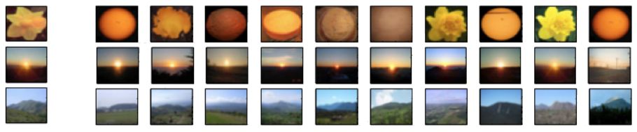
One way to approach this problem is to formalize it as the -medoid problem. Given a set of images (called ground set) associated with a (not necessarily symmetric) dissimilarity function, we seek to select a subset of at most exemplars or cluster centers, and then assign each image in the dataset to its least dissimilar exemplar. If an element is assigned to exemplar , then the cost associated with is the dissimilarity between and . The goal of the -medoid problem is to choose exemplars that minimize the sum of dissimilarities between every data point and its assigned cluster center.
Solving the -medoid problem optimally is NP-hard, however, as we discuss in Section 3.4, we can transform this problem, and many other summarization tasks, to the problem of maximizing a monotone submodular function subject to a cardinality constraint
| (1) |
Submodular functions are set functions which satisfy the following natural diminishing returns property.
Definition 1 (c.f., Nemhauser et al. (1978)).
A set function is submodular, if for every and
Furthermore, is called monotone iff for all it holds that .
We will generally additionally require that is nonnegative, i.e., for all sets .
Problem (1) is NP-hard for many classes of submodular functions (Feige, 1998). A fundamental result by Nemhauser et al. (1978) establishes that a simple greedy algorithm that starts with the empty set and iteratively augments the current solution with an element of maximum incremental value
| (2) |
continuing until elements have been selected, is guaranteed to provide a constant factor approximation.
Theorem 2.
(Nemhauser et al., 1978) For any non-negative and monotone submodular function , the greedy heuristic always produces a solution of size that achieves at least a constant factor of the optimal solution.
This result can be easily extended to , where and are two positive integers (Krause and Golovin, 2012, see,).
3.2 Distributed Submodular Maximization
In many today’s applications where the size of the ground set is very large and cannot be stored on a single computer, running the standard greedy algorithm or its variants (Minoux, 1978; Leskovec et al., 2007; Mirzasoleiman et al., 2015a, e.g., lazy evaluations,) in a centralized manner is infeasible. Hence, we seek a solution that is suitable for large-scale parallel computation. The greedy method described above is in general difficult to parallelize, since it is inherently sequential: at each step, only the object with the highest marginal gain is chosen and every subsequent step depends on the preceding ones.
Concretely, we consider the setting where the ground set is very large and cannot be handled on a single machine, thus must be distributed among a set of machines. While there are several approaches towards parallel computation, in this paper we consider the following model that can be naturally implemented in MapReduce. The computation proceeds in a sequence of rounds. In each round, the dataset is distributed to machines. Each machine carries out computations independently in parallel on its local data. After all machines finish, they synchronize by exchanging a limited amount of data (of size polynomial in and , but independent of ). Hence, any distributed algorithm in this model must specify: 1) how to distribute among the machines, 2) which algorithm should run on each machine, and 3) how to communicate and merge the resulting solutions.
In particular, the distributed submodular maximization problem requires the specification of the above steps in order to implement an approach for submodular maximization. More precisely, given a monotone submodular function , a cardinality constraint , and a number of machines , we wish to produce a solution of size such that is competitive with the optimal centralized solution .
3.3 Naive Approaches Towards Distributed Submodular Maximization
One way to solve problem (1) in a distributed fashion is as follows. The dataset is first partitioned (randomly, or using some other strategy) onto the machines, with representing the data allocated to machine . We then proceed in rounds. In each round, all machines–in parallel–compute the marginal gains of all elements in their sets . Next, they communicate their candidate to a central processor, who identifies the globally best element, which is in turn communicated to the machines. This element is then taken into account for computing the marginal gains and selecting the next elements. This algorithm (up to decisions on how break ties) implements exactly the centralized greedy algorithm, and hence provides the same approximation guarantees on the quality of the solution. Unfortunately, this approach requires synchronization after each of the rounds. In many applications, is quite large (e.g., tens of thousands), rendering this approach impractical for MapReduce style computations.
An alternative approach for large would be to greedily select elements independently on each machine (without synchronization), and then merge them to obtain a solution of size . This approach that requires only two rounds (as opposed to ), is much more communication efficient, and can be easily implemented using a single MapReduce stage. Unfortunately, many machines may select redundant elements, and thus the merged solution may suffer from diminishing returns. It is not hard to construct examples for which this approach produces solutions that are a factor worse than the centralized solution.
In Section 4, we introduce an alternative protocol GreeDi, which requires little communication, while at the same time yielding a solution competitive with the centralized one, under certain natural additional assumptions.
3.4 Applications of Distributed Submodular Maximization
In this part, we discuss two concrete problem instances, with their corresponding submodular objective functions , where the size of the datasets often requires a distributed solution for the underlying submodular maximization.
3.4.1 Large-scale Nonparametric Learning
Nonparametric learning (i.e., learning of models whose complexity may depend on the dataset size ) are notoriously hard to scale to large datasets. A concrete instance of this problem arises from training Gaussian processes or performing MAP inference in Determinantal Point Processes, as considered below. Similar challenges arise in many related learning methods, such as training kernel machines, when attempting to scale them to large data sets.
Active Set Selection in Sparse Gaussian Processes (GPs). Formally a GP is a joint probability distribution over a (possibly infinite) set of random variables , indexed by the ground set , such that every (finite) subset for is distributed according to a multivariate normal distribution. More precisely, we have
where and are prior mean and covariance matrix, respectively. The covariance matrix is parametrized via a positive definite kernel . As a concrete example, when elements of the ground set are embedded in a Euclidean space, a commonly used kernel in practice is the squared exponential kernel defined as follows:
Gaussian processes are commonly used as priors for nonparametric regression. In GP regression, each data point is considered a random variable. Upon observations (where is a vector of independent Gaussian noise with variance ), the predictive distribution of a new data point is a normal distribution , where mean and variance are given by
| (3) | ||||
| (4) |
Evaluating (3) and (4) is computationally expensive as it requires solving a linear system of variables. Instead, most efficient approaches for making predictions in GPs rely on choosing a small–so called active–set of data points. For instance, in the Informative Vector Machine (IVM) one seeks a set such that the information gain, defined as
is maximized. It can be shown that this choice of is monotone submodular (Krause and Guestrin, 2005a). For medium-scale problems, the standard greedy algorithms provide good solutions. For massive data however, we need to resort to distributed algorithms. In Section 6, we will show how GreeDi can choose near-optimal subsets out of a dataset of 45 million vectors.
Inference for Determinantal Point Processes. A very similar problem arises when performing inference in Determinantal Point Processes (DPPs). DPPs (Macchi, 1975) are distributions over subsets with a preference for diversity, i.e., there is a higher probability associated with sets containing dissimilar elements. Formally, a point process on a set of items is a probability measure on (the set of all subsets of ). is called determinantal point process if for every we have:
where is a positive semidefinite kernel matrix, and , is the restriction of to the entries indexed by elements of (we adopt that ). The normalization constant can be computed explicitly from the following equation
where is the identity matrix. Intuitively, the kernel matrix determines which items are similar and therefore less likely to appear together.
In order to find the most diverse and informative subset of size , we need to find which is NP-hard, as the total number of possible subsets is exponential (Ko et al., 1995). However, the objective function is log-submodular, i.e. is a submodular function (Kulesza, 2012). Hence, MAP inference in large DPPs is another potential application of distributed submodular maximization.
3.4.2 Large-scale Exemplar Based Clustering
Suppose we wish to select a set of exemplars, that best represent a massive dataset. One approach for finding such exemplars is solving the -medoid problem (Kaufman and Rousseeuw, 2009), which aims to minimize the sum of pairwise dissimilarities between exemplars and elements of the dataset. More precisely, let us assume that for the dataset we are given a nonnegative function (not necessarily assumed symmetric, nor obeying the triangle inequality) such that encodes dissimilarity between elements of the underlying set . Then, the cost function for the -medoid problem is:
| (5) |
Finding the subset
of cardinality at most that minimizes the cost function (5) is NP-hard. However, by introducing an auxiliary element , a.k.a. phantom exemplar, we can turn into a monotone submodular function (Krause and Gomes, 2010)
| (6) |
In words, measures the decrease in the loss associated with the set versus the loss associated with just the auxiliary element. We begin with a phantom exemplar and try to find the active set that together with the phantom exemplar reduces the value of our loss function more than any other set. Technically, any point that satisfies the following condition can be used as a phantom exemplar:
This condition ensures that once the distance between any and is greater than the maximum distance between elements in the dataset, then . As a result, maximizing (a monotone submodular function) is equivalent to minimizing the cost function . This problem becomes especially computationally challenging when we have a large dataset and we wish to extract a manageable-size set of exemplars, further motivating our distributed approach.
3.4.3 Other Examples
Numerous other real world problems in machine learning can be modeled as maximizing a monotone submodular function subject to appropriate constraints (e.g., cardinality, matroid, knapsack). To name a few, specific applications that have been considered range from efficient content discovery for web crawlers and multi topic blog-watch (Chierichetti et al., 2010), over document summarization (Lin and Bilmes, 2011) and speech data subset selection (Wei et al., 2013), to outbreak detection in social networks (Leskovec et al., 2007), online advertising and network routing (De Vries and Vohra, 2003), revenue maximization in social networks (Hartline et al., 2008), and inferring network of influence (Gomez Rodriguez et al., 2010). In all such examples, the size of the dataset (e.g., number of webpages, size of the corpus, number of blogs in the blogosphere, number of nodes in social networks) is massive, thus GreeDi offers a scalable approach, in contrast to the standard greedy algorithm, for such problems.
4 The GreeDi Approach for Distributed Submodular Maximization
In this section we present our main results. We first provide our distributed solution GreeDi for maximizing submodular functions under cardinality constraints. We then show how we can make use of the geometry of data inherent in many practical settings in order to obtain strong data-dependent bounds on the performance of our distributed algorithm.
4.1 An Intractable, yet Communication Efficient Approach
Before we introduce GreeDi, we first consider an intractable, but communication–efficient two-round parallel protocol to illustrate the ideas. This approach, shown in Algorithm 1, first distributes the ground set to machines. Each machine then finds the optimal solution, i.e., a set of cardinality at most , that maximizes the value of in each partition. These solutions are then merged, and the optimal subset of cardinality is found in the combined set. We denote this distributed solution by .
As the optimum centralized solution achieves the maximum value of the submodular function, it is clear that . For the special case of selecting a single element , we have . Furthermore, for modular functions (i.e., those for which and are both submodular), it is easy to see that the distributed scheme in fact returns the optimal centralized solution as well. In general, however, there can be a gap between the distributed and the centralized solution. Nonetheless, as the following theorem shows, this gap cannot be more than . Furthermore, this result is tight.
Theorem 3.
Let be a monotone submodular function and let . Then, . In contrast, for any value of and , there is a monotone submodular function such that .
The proof of all the theorems can be found in the appendix. The above theorem fully characterizes the performance of Algorithm 1 in terms of the best centralized solution. In practice, we cannot run Algorithm 1, since there is no efficient way to identify the optimum subset in set , unless P=NP. In the following, we introduce an efficient distributed approximation – GreeDi. We will further show, that under some additional assumptions, much stronger guarantees can be obtained.
4.2 Our GreeDi Approximation
Our efficient distributed method GreeDi is shown in Algorithm 2. It parallels the intractable Algorithm 1, but replaces the selection of optimal subsets, i.e., , by greedy solutions . Due to the approximate nature of the greedy algorithm, we allow it to pick sets slightly larger than . More precisely, GreeDi is a two-round algorithm that takes the ground set , the number of partitions , and the cardinality constraint . It first distributes the ground set over machines. Then each machine separately runs the standard greedy algorithm by sequentially finding an element that maximizes the discrete derivative (2). Each machine –in parallel–continues adding elements to the set until it reaches elements. We define to be the set with the maximum value among . Then the solutions are merged, i.e., , and another round of greedy selection is performed over until elements are selected. We denote this solution by . The final distributed solution with parameters and , denoted by , is the set with a higher value between and (c.f., Figure 2 shows GreeDi schematically). The following result parallels Theorem 3.
Theorem 4.
Let be a monotone submodular function and . Then
For the special case of the result of 4 simplifies to . Moreover, it is straightforward to generalize GreeDi to multiple rounds (i.e., more than two) for very large datasets.
In light of Theorem 3, one can expect that in general it is impossible to eliminate the dependency of the distributed solution on 11 1 It has been very recently shown by Mirzasoleiman et al. (2015b) that the tightest dependency is .. However, as we show in the sequel, in many practical settings, the ground set exhibits rich geometrical structure that can be used to obtain stronger guarantees.
4.3 Performance on Datasets with Geometric Structure
In practice, we can hope to do much better than the worst case bounds shown previously by exploiting underlying structure often present in real data and important set functions. In this part, we assume that a metric exists on the data elements, and analyze performance of the algorithm on functions that vary slowly with changes in the input. We refer to these as Lipschitz functions:
Definition 5.
Let . A set function is -Lipschitz w.r.t. metric on , if for any integer , any equal sized sets and and any matching of elements: , the difference between and is bounded by:
| (7) |
We can show that the objective functions from both examples in Section 3.4 are -Lipschitz for suitable kernels/distance functions:
Proposition 6.
Suppose that the covariance matrix of a Gaussian process is parametrized via a positive definite kernel which is Lipschitz continuous with respect to metric with constant , i.e., for any triple of points , we have . Then, the mutual information for the Gaussian process is -Lipschitz with , where is the number of elements in the selected subset .
Proposition 7.
Let be a metric on the elements of the dataset. Furthermore, let encode the dissimilarity between elements of the underlying set . Then for , the loss function (and hence also the corresponding submodular utility function ) is -Lipschitz with , where is the diameter of the ball encompassing elements of the dataset in the metric space. In particular, for the -medoid problem, which minimizes the loss function over all clusters with respect to , we have , and for the -means problem, which minimizes the loss function over all clusters with respect to , we have .
Beyond Lipschitz-continuity, many practical instances of submodular maximization can be expected to satisfy a natural density condition. Concretely, whenever we consider a representative set (i.e., optimal solution to the submodular maximization problem), we expect that any of its constituent elements has potential candidates for replacement in the ground set. For example, in our exemplar-based clustering application, we expect that cluster centers are not isolated points, but have many almost equally representative points close by. Formally, for any element , we define its -neighborhood as the set of elements in within distance from (i.e., -close to ):
By -Lipschitz-continuity, it must hold that if we replace element in set by an -close element (i.e., ) to get a new set of equal size, it must hold that .
As described earlier, our algorithm GreeDi partitions into sets for parallel processing. If in addition we assume that elements are assigned uniformly at random to different machines, -neighborhoods are sufficiently dense, and the submodular function is Lipschitz continuous, then GreeDi is guaranteed to produce a solution close to the centralized one. More formally, we have the following theorem.
Theorem 8.
Under the conditions that 1) elements are assigned uniformly at random to machines, 2) for each we have , and 3) is -Lipschitz continuous, then with probability at least the following holds:
Note that once the above conditions are satisfied for small values of (meaning that there is a high density of data points within a small distance from each element of the optimal solution) then the distributed solution will be close to the optimal centralized one. In particular if we let , the distributed solution is guaranteed to be within a factor from the optimal centralized solution. This situation naturally corresponds to very large datasets. In the following, we discuss more thoroughly this important scenario.
4.4 Performance Guarantees for Very Large Datasets
Suppose that our dataset is a finite sample drawn i.i.d. from an underlying infinite set , according to some (unknown) probability distribution. Let be an optimal solution in the infinite set, i.e., , such that around each , there is a neighborhood of radius at least where the probability density is at least at all points (for some constants and ). This implies that the solution consists of elements coming from reasonably dense and therefore representative regions of the dataset.
Let us suppose is the growth function of the metric: is defined to be the volume of a ball of radius centered at a point in the metric space. This means, for the probability of a random element being in is at least and the expected number of neighbors of is at least . As a concrete example, Euclidean metrics of dimension have . Note that for simplicity we are assuming the metric to be homogeneous, so that the growth function is the same at every point. For heterogeneous spaces, we require to have a uniform lower bound on the growth function at every point.
In these circumstances, the following theorem guarantees that if the dataset is sufficiently large and is -Lipschitz, then GreeDi produces a solution close to the centralized one.
Theorem 9.
For , where , if the algorithm GreeDi assigns elements uniformly randomly to processors , then with probability at least ,
The above theorem shows that for very large datasets, GreeDi provides a solution that is within a factor of the optimal centralized solution. This result is based on the fact that for sufficiently large datasets, there is a suitably dense neighborhood around each member of the optimal solution. Thus, if the elements of the dataset are partitioned uniformly randomly to processors, at least one partition contains a set such that its elements are very close to the elements of the optimal centralized solution and provides a constant factor approximation of the optimal centralized solution.
4.5 Handling Decomposable Functions
So far, we have assumed that the objective function is given to us as a black box, which we can evaluate for any given set independently of the dataset . In many settings, however, the objective depends itself on the entire dataset. In such a setting, we cannot use GreeDi as presented above, since we cannot evaluate on the individual machines without access to the full set . Fortunately, many such functions have a simple structure which we call decomposable. More precisely, we call a submodular function decomposable if it can be written as a sum of submodular functions as follows (Krause and Gomes, 2010):
In other words, there is separate submodular function associated with every data point . We require that each can be evaluated without access to the full set . Note that the exemplar based clustering application we discussed in Section 3.4 is an instance of this framework, among many others. Let us define the evaluation of restricted to as follows:
In the remaining of this section, we show that assigning each element of the dataset randomly to a machine and running GreeDi will provide a solution that is with high probability close to the optimum solution. For this, let us assume that ’s are bounded, and without loss of generality for . Similar to Section 4.3 we assume that GreeDi performs the partition by assigning elements uniformly at random to the machines. These machines then each greedily optimize . The second stage of GreeDi optimizes , where is chosen uniformly at random with size .
Then, we can show the following result. First, for any fixed , let us define to be the smallest integer such that for we have .
Theorem 10.
For , , and under the assumptions of Theorem 9, we have, with probability at least ,
The above result demonstrates why GreeDi performs well on decomposable submodular functions with massive data even when they are evaluated locally on each machine. We will report our experimental results on exemplar-based clustering in the next section.
4.6 Performance of GreeDi on Random Partitions Without Geometric Structure
Very recently, a constant -approximation guarantee was proven for GreeDi for the case of random partitioning of the data among the machines.
Theorem 11 (Barbosa et al. (2015); Mirrokni and Zadimoghaddam (2015)).
If elements are assigned uniformly at random to the machines, and , GreeDi gives a approximation guarantee (in the average case) to the optimum centralized solution.
These results show that random partitioning of the data is sufficient to guarantee that GreeDi provides a constant factor approximation, irrespective of and , and without the requirement of any geometric structure. On the other hand, if geometric structure is present, the bounds from the previous sections can provide sharper approximation guarantees.
5 (Non-Monotone) Submodular Functions with General Constraints
In this section we show how GreeDi can be extended to handle 1) more general constraints, and 2) non-monotone submodular functions. More precisely, we consider the following optimization setting
Here, we assume that the feasible solutions should be members of the constraint set . The function is submodular but may not be monotone. By overloading the notation we denote the set that achieves the above constrained optimization problem by . Throughout this section we assume that the constraint set is hereditary, meaning that if then for any we also require that . Cardinality constraints are obviously hereditary, so are all the examples we mention below.
5.1 Matroid Constraints
A matroid is a pair where is a finite set (called the ground set) and is a family of subsets of (called the independent sets) satisfying the following two properties:
- •
Heredity property: and implies that , i.e. every subset of an independent set is independent.
- •
Augmentation property: If and , there is an element such that .
Maximizing a submodular function subject to matroid constraints has found several applications in machine learning and data mining, ranging from content aggregation on the web (Abbassi et al., 2013) to viral marketing (Narayanam and Nanavati, 2012) and online advertising (Streeter et al., 2009).
One way to approximately maximize a monotone submodular function subject to the constraint that each is independent, i.e., , is to use a generalization of the greedy algorithm. This algorithm, which starts with an empty set and in each iteration picks the feasible element with maximum benefit until there is no more element such that , is guaranteed to provide a -approximation of the optimal solution (Fisher et al., 1978). Recently, this bound has been improved to using the continuous greedy algorithm (Calinescu et al., 2011). For non-negative and non-monotone submodular functions with matroid constraints, the best known result is a 0.325-approximation based on simulated annealing (Gharan and Vondrák, 2011).
Curvature:
For a submodular function , the total curvature of with respect to a set is defined as:
Intuitively, the notion of curvature determines how far away is from being modular. In other words, it measures how much the marginal gain of an element w.r.t. set can decrease as a function of . In general, , and for additive (modular) functions, , i.e., the marginal values are independent of . In this case, the greedy algorithm returns the optimal solution to . In general, the greedy algorithm gives a -approximation to maximizing a non-decreasing submodular function with curvature subject to a matroid constraint (Conforti and Cornuéjols, 1984). In case of the uniform matroid , the approximation factor is .
Intersection of Matroids:
A more general case is when we have matroids on the same ground set , and we want to maximize the submodular function on the intersection of matroids. That is, consists of all subsets of that are independent in all matroids. This constraint arises, e.g., when optimizing over rankings (which can be modeled as intersections of two partition matroids). Another recent application considered is finding the influential set of users in viral marketing when multiple products need to be advertised and each user can tolerate only a small number of recommendations (Du et al., 2013). For matroid constraints, the -approximation provided by the greedy algorithm (Fisher et al., 1978) has been improved to a -approximation for by Lee et al. (2009b). For the non-monotone case, a -approximation based on local search is also given by Lee et al. (2009b) .
-systems:
-independence systems generalize constraints given by the intersection of matroids. Given an independence family and a set , let denote the set of maximal independent sets of included in , i.e., . Then we call a -system if for all nonempty we have
Similar to matroid constraints, the greedy algorithm provides a -approximation guarantee for maximizing a monotone submodular function subject to a -systems constraint (Fisher et al., 1978). For the non-monotone case, a -approximation can be achieved by combining an algorithm of Gupta et al. (2010) with the result for unconstrained submodular maximization of Buchbinder et al. (2012).
5.2 Knapsack Constraints
In many applications, including feature and variable selection in probabilistic models (Krause and Guestrin, 2005a) and document summarization (Lin and Bilmes, 2011), elements have non-uniform costs , and we wish to find a collection of elements that maximize subject to the constraint that the total cost of elements in does not exceed a given budget , i.e.
Since the simple greedy algorithm ignores cost while iteratively adding elements with maximum marginal gains according (see Eq. 2) until , it can perform arbitrary poorly. However, it has been shown that taking the maximum over the solution returned by the greedy algorithm that works according to Eq. 2 and the solution returned by the modified greedy algorithm that optimizes the cost-benefit ratio
provides a -approximation of the optimal solution (Krause and Guestrin, 2005b). Furthermore, a more computationally expensive algorithm which starts with all feasible solutions of cardinality 3 and augments them using the cost-benefit greedy algorithm to find the set with maximum value of the objective function provides a -approximation (Sviridenko, 2004). For maximizing non-monotone submodular functions subject to knapsack constraints, a ()-approximation algorithm based on local search was given by Lee et al. (2009a).
Multiple Knapsack Constraints:
In some applications such as procurement auctions (Garg et al., 2001), video-on-demand systems and e-commerce (Kulik et al., 2009), we have a -dimensional budget vector and a set of element where each element is associated with a -dimensional cost vector. In this setting, we seek a subset of elements with a total cost of at most that maximizes a non-decreasing submodular function . Kulik et al. (2009) proposed a two-phase algorithm that provides a -approximation for the problem by first guessing a constant number of elements of highest value, and then taking the value residual problem with respect to the guessed subset. For the non-monotone case, Lee et al. (2009a) provided a -approximation based on local search.
-system and knapsack constraints:
A more general type of constraint that has recently found interesting applications in viral marketing (Du et al., 2013) can be constructed by combining a -system with knapsack constraints which comprises the intersection of matroids or knapsacks as special cases. Badanidiyuru and Vondrák (2014) proposed a modified version of the greedy algorithm that guarantees a -approximation for maximizing a monotone submodular function subject to -system and knapsack constraints.
Table 1 summarizes the approximation guarantees for monotone and non-monotone submodular maximization under different constraints.
| Constraint | Approximation () | |
|---|---|---|
| monotone submodular functions | non-monotone submodular functions | |
| Cardinality | (Fisher et al., 1978) | 0.325 (Gharan and Vondrák, 2011) |
| 1 matroid | (Calinescu et al., 2011) | 0.325 (Gharan and Vondrák, 2011) |
| matroid | (Lee et al., 2009b) | (Lee et al., 2009b) |
| 1 knapsack | (Sviridenko, 2004) | 1/5 - (Lee et al., 2009a) |
| knapsack | Kulik et al. (2009) | 1/5 - (Lee et al., 2009a) |
| -system | 1/() (Fisher et al., 1978) | (Gupta et al., 2010) |
| -system + knapsack | (Badanidiyuru and Vondrák, 2014) | – |
5.3 GreeDi Approximation Guarantee under More General Constraints
Assume that we have a set of constraints that is hereditary. Further assume we have access to a ”black box” algorithm that gives us a constant factor approximation guarantee for maximizing a non-negative (but not necessarily monotone) submodular function subject to , i.e.
| (8) |
We can modify GreeDi to use any such approximation algorithm as a black box, and provide theoretical guarantees about the solution. In order to process a large dataset, it first distributes the ground set over machines. Then instead of greedily selecting elements, each machine –in parallel–separately runs the black box algorithm on its local data in order to produce a feasible set meeting the constraints . We denote by the set with maximum value among . Next, the solutions are merged: , and the black box algorithm is applied one more time to set to produce a solution . Then, the distributed solution for parameter and constraints , , is the best among and . This procedure is given in more detail in Algorithm 3.
The following result generalizes Theorem 4 for maximizing a submodular function subject to more general constraints.
Theorem 12.
Let be a non-negative submodular function and be a black box algorithm that provides a -approximation guarantee for submodular maximization subject to a set of hereditary constraints . Then
where is the optimum centralized solution, and .
Specifically, for submodular maximization subject to the matroid constraint , we have where is the rank of the matroid (i.e., the maximum size of any independent set in the system). For submodular maximization subject to the knapsack constraint , we can bound by (i.e. the capacity of the knapsack divided by the smallest weight of any element).
Performance on Datasets with Geometric Structure.
When the submodular function and the constraint set have more structure, then we can provide much better approximation guarantees. Assuming the elements of are embedded in metric space with distance , we say that is locally replaceable with respect to a set with parameter if
Here, we define the distance between two sets and of the same size as follows. Let be the set of all possible matchings between and , i.e.,
Then . We require locality only with respect to to ensure that the optimum solution can be well approximated. What the locally replaceable property requires is that as elements of get replaced by nearby elements, the resulting set is also a feasible solution. Combining this property with -Lipschitzness will provide us with the following theorem.
Theorem 13.
Under the conditions that 1) elements are assigned uniformly at random to machines, 2) for each we have , 3) is -Lipschitz, and 4) is locally replaceable with respect to with parameter , then with probability at least ,
The above result generalizes Theorem 8 for maximizing non-negative submodular functions subject to different constraints.
Performance Guarantee for Very Large datasets.
Similarly, we can generalize Theorem 9 for maximizing non-negative submodular functions subject to more general constraints. Suppose that our dataset is a finite sample drawn i.i.d. from an underlying infinite set , according to some (unknown) probability distribution. Let be an optimal solution in the infinite set, i.e., , such that around each , there is a neighborhood of radius at least where the probability density is at least at all points (for some constants and ). Recall that is the growth function where measures the volume of a ball of radius centered at a point in the metric space.
Theorem 14.
For , where , if GreeDi assigns elements uniformly at random to processors and under the conditions that is -Lipschitz, and is locally replaceable with respect to with parameter , then with probability at least , we have
Performance Guarantee for Decomposable Functions.
For the case of decomposable functions described in Section 4.5, the following generalization of Theorem 10 holds for maximizing a non-negative submodular function subject to more general constraints. Let us define to be the smallest integer such that for we have .
Theorem 15.
For , , and under the assumptions of Theorem 14, we have, with probability at least ,
6 Experiments
In our experimental evaluation we wish to address the following questions: 1) how well does GreeDi perform compared to the centralized solution, 2) how good is the performance of GreeDi when using decomposable objective functions (see Section 4.5), and finally 3) how well does GreeDi scale in the context of massive datasets. To this end, we run GreeDi on three scenarios: exemplar based clustering, active set selection in GPs and finding the maximum cuts in graphs.
We compare the performance of our GreeDi method to the following naive approaches:
- •
random/random: in the first round each machine simply outputs randomly chosen elements from its local data points and in the second round out of the merged elements, are again randomly chosen as the final output.
- •
random/greedy: each machine outputs randomly chosen elements from its local data points, then the standard greedy algorithm is run over elements to find a solution of size .
- •
greedy/merge: in the first round elements are chosen greedily from each machine and in the second round they are merged to output a solution of size .
- •
greedy/max: in the first round each machine greedily finds a solution of size and in the second round the solution with the maximum value is reported.
For GreeDi, we let each of the machines select a set of size , and select a final solution of size among the union of the solutions (i.e., among elements). We present the performance of GreeDi for different parameters . For datasets where we are able to find the centralized solution, we report the ratio of , where is the distributed solution (in particular for GreeDi).
6.1 Exemplar Based Clustering
Our exemplar based clustering experiment involves GreeDi applied to the clustering utility (see Sec. 3.4) with . We performed our experiments on a set of 10,000 Tiny Images (Torralba et al., 2008). Each 32 by 32 RGB pixel image was represented by a 3,072 dimensional vector. We subtracted from each vector the mean value, normalized it to unit norm, and used the origin as the auxiliary exemplar. Fig. 4(a) compares the performance of our approach to the benchmarks with the number of exemplars set to , and varying number of partitions . It can be seen that GreeDi significantly outperforms the benchmarks and provides a solution that is very close to the centralized one. Interestingly, even for very small , GreeDi performs very well. Since the exemplar based clustering utility function is decomposable, we repeated the experiment for the more realistic case where the function evaluation in each machine was restricted to the local elements of the dataset in that particular machine (rather than the entire dataset). Fig 4(b) shows similar qualitative behavior for decomposable objective functions.
Large scale experiments with Hadoop. As our first large scale experiment, we applied GreeDi to the whole dataset of 80,000,000 Tiny Images (Torralba et al., 2008) in order to select a set of 64 exemplars. Our experimental infrastructure was a cluster of 10 quad-core machines running Hadoop with the number of reducers set to . Hereby, each machine carried out a set of reduce tasks in sequence. We first partitioned the images uniformly at random to reducers. Each reducer separately performed the lazy greedy algorithm on its own set of 10,000 images (123MB) to extract 64 images with the highest marginal gains w.r.t. the local elements of the dataset in that particular partition. We then merged the results and performed another round of lazy greedy selection on the merged results to extract the final 64 exemplars. Function evaluation in the second stage was performed w.r.t a randomly selected subset of 10,000 images from the entire dataset. The maximum running time per reduce task was 2.5 hours. As Fig. 5(a) shows, GreeDi highly outperforms the other distributed benchmarks and can scale well to very large datasets. Fig. 5(b) shows a set of cluster exemplars discovered by GreeDi where Fig. 5(c) and Fig. 5(d) show 100 nearest images to exemplars 26 and 63 (shown with red borders) in Fig. 5(b).


6.2 Active Set Selection
Our active set selection experiment involves GreeDi applied to the information gain (see Sec. 3.4) with Gaussian kernel, and . We used the Parkinsons Telemonitoring dataset (Tsanas et al., 2010) consisting of 5,875 bio-medical voice measurements with 22 attributes from people with early-stage Parkinson’s disease. We normalized the vectors to zero mean and unit norm. Fig. 6(b) compares the performance GreeDi to the benchmarks with fixed and varying number of partitions . Similarly, Fig 6(a) shows the results for fixed and varying . We find that GreeDi significantly outperforms the benchmarks.
Large scale experiments with Hadoop. Our second large scale experiment consists of 45,811,883 user visits from the Featured Tab of the Today Module on Yahoo! Front Page (web, 2012). For each visit, both the user and each of the candidate articles are associated with a feature vector of dimension 6. Here, we used the normalized user features. Our experimental setup was a cluster of 8 quad-core machines running Spark with the number of reducers set to . Each reducer performed the lazy greedy algorithm on its own set of 1,431,621 vectors (34MB) in order to extract 256 elements with the highest marginal gains w.r.t the local elements of the dataset in that particular partition. We then merged the results and performed another round of lazy greedy selection on the merged results to extract the final active set of size 256. The maximum running time per reduce task was 12 minutes for selecting 128 elements and 48 minutes for selecting 256 elements. Fig. 7 shows the performance of GreeDi compared to the benchmarks. We note again that GreeDi significantly outperforms the other distributed benchmarks and can scale well to very large datasets.
Performance Comparison. Fig. 8 shows the speedup of GreeDi compared to the centralized greedy benchmark for different values of and varying number of partitions . As Fig. 8(a) shows, for small values of , the speedup is almost linear in the number of machines. However, for large values of the running time of the second stage of GreeDi increases and ultimately dominates the whole running time. Hence, we do not observe a linear speedup anymore. This effect can be observed in Fig. 8(b). For larger values of , the speedup is higher on fewer machines, but decreases more quickly by increasing , as the second stage takes longer to complete.
6.3 Non-Monotone Submodular Function (Finding Maximum Cuts)
We also applied GreeDi to the problem of finding maximum cuts in graphs. In our setting we used a Facebook-like social network (Opsahl and Panzarasa, 2009). This dataset includes the users that have sent or received at least one message in an online student community at University of California, Irvine and consists of 1,899 users and 20,296 directed ties. Fig. 9(a) and 9(b) show the performance of GreeDi applied to the cut function on graphs. We evaluated the objective function locally on each partition. Thus, the links between the partitions are disconnected. Since the problem of finding the maximum cut in a graph is non-monotone submodular, we applied the RandomGreedy algorithm proposed by Buchbinder et al. (2014) to find the near optimal solution in each partition.
Although the cut function does not decompose additively over individual data points, perhaps surprisingly, GreeDi still performs very well, and significantly outperforms the benchmarks. This suggests that our approach is quite robust, and may be more generally applicable.
6.4 Comparision with Greedy Scaling.
Kumar et al. (2013) recently proposed an alternative approach–GreedyScaling–for parallel maximization of submodular functions. GreedyScaling is a randomized algorithm that carries out a number (typically less than ) rounds of MapReduce computations. We applied GreeDi to the submodular coverage problem in which given a collection of sets, we would like to pick at most sets from in order to maximize the size of their union. We compared the performance of our GreeDi algorithm to the reported performance of GreedyScaling on the same datasets, namely Accidents (Geurts et al., 2003) and Kosarak (Bodon, 2012). As Fig 10(a) and 10(b) shows, GreeDi outperforms GreedyScaling on the Accidents dataset and its performance is comparable to that of GreedyScaling in the Kosarak dataset.
7 Conclusion
We have developed an efficient distributed protocol GreeDi, for constrained submodular function maximization. We have theoretically analyzed the performance of our method and showed that under certain natural conditions it performs very close to the centralized (albeit impractical in massive datasets) solution. We have also demonstrated the effectiveness of our approach through extensive experiments, including active set selection in GPs on a dataset of 45 million examples, and exemplar based summarization of a collection of 80 million images using Hadoop. We believe our results provide an important step towards solving submodular optimization problems in very large scale, real applications.
acknowledgments-disclosure-of-funding.
This research was supported by SNF 200021-137971, DARPA MSEE FA8650-11-1-7156, ERC StG 307036, a Microsoft Faculty Fellowship, an ETH Fellowship, and a Scottish Informatics and Computer Science Alliance.Appendix A Proofs
This section presents the complete proofs of theorems presented in the article.
A.1 Proof of Theorem 3
direction:
The proof easily follows from the following lemmas.
Lemma 16.
.
Proof.
Let be the elements in that are contained in the optimal solution, . Then we have:
Using submodularity of , for each , we have
and thus,
Since, , we have
Therefore,
∎
Lemma 17.
.
Proof.
Let . Using submodularity of , we have
Thus, where . Suppose that the element with highest marginal gain (i.e., ) is in . Then the maximum value of on would be greater or equal to the marginal gain of , i.e., and since , we can conclude that
∎
direction:
Let us consider a set of unbiased and independent Bernoulli random variables for and , i.e., and if or . Let us also define for . Now assume that and , where is the entropy of the subset of random variables. Note that is a monotone submodular function. It is easy to see that or as in both cases . If we assume , then . Hence, by selecting at most elements from , we have . On the other hand, the set of elements that maximizes the entropy is . Note that and for . Hence, if or otherwise .
A.2 Proof of Theorem 4
Let us first mention a slight generalization over the performance of the standard greedy algorithm. It follows easily from the argument in (Nemhauser et al., 1978).
Lemma 18.
Let be a non-negative submodular function, and let of cardinality be the greedy selected set by the standard greedy algorithm. Then,
A.3 Proof of Proposition 6
Let be a positive definite kernel matrix defined in section 3.4.1. If we replace a point with another point , the corresponding row and column in the modified kernel matrix will be changed. W.l.o.g assume that we replace the first element with another element , i.e., has the following form with non-zero entries only on the first row and first column,
Note that kernel is Lipschitz continuous with constant , hence we have for . Then the absolute value of the change in the objective function would be
| (9) |
Note that since is positive-definite, is an invertible matrix. Furthermore, since and are symmetric matrices they both have real eigenvalues. Therefore, has eigenvalues , for , where are (non-negative) eigenvalues of kernel matrix .
Now, we bound the maximum eigenvalues of and respectively. Consider vectors , such that . We have,
| (10) |
where we used the following facts to derive the last inequality: 1) the Lipschitz continuity of the kernel gives us an upperbound on the values of , i.e., for ; and 2) since , the absolute value of the elements in vectors and cannot be greater than 1, i.e., , for . Therefore,
Now, let be the eigenvectors of matrix . Note that is an orthonormal system and thus for any we can write it as , and we have . In order to bound the largest eigenvalue of , we write
where in (a) we used Eq. 10 and the fact that for . Using Cauchy-Schwarz inequality
and the assumption , we conclude
Therefore,
| (11) |
Finally, we can write the determinant of a matrix as the product of its eigenvalues, i.e.
| (12) |
Replacing all the points in set with another set of the same size, we get
Hence, the differential entropy of the Gaussian process is -Lipschitz with .
A.4 Proof of Proposition 7
Assume we have a set of exemplars, i.e., , and each element of the dataset is assigned to its closest exemplar. Now, if we replace set with another set of the same size, the loss associated with every element may be changed. W.l.o.g, assume we swap one exemplar at a time, i.e., in step , we have . Swapping the exemplar with another element , 4 cases may happen: 1) element was not assigned to before and doesn’t get assigned to , 2) element was assigned to before and gets assigned to , 3) element was not assigned to before and gets assigned to , 4) element was assigned to before and gets assigned to another exemplar . For any element , we look into the four cases and show that in each case
- •
Case 1: In this case, element was assigned to another exemplar and the assignment doesn’t change. Therefore, there is no change in the value of the loss function.
- •
Case 2: In this case, element was assigned to before and gets assigned to . let and . Then we can write
(13) where in the last step we used triangle inequality and the fact that data points are in a ball of diameter in the metric space.
- •
Case 3: In this case, was assigned to another exemplar and gets assigned to , which implies that , since otherwise would have been assigned to before.
- •
Case 4: In the last case, element was assigned to before and gets assigned to another exemplar . Thus, we have since otherwise would have been assigned to before. Hence, in all four cases the following inequality holds:
By using Eq. 13 and averaging over all elements , we have
Thus, for any point that satisfies
we have and thus
Now, if we replace all the points in set with another set of the same size, we get
Therefore, for , the loss function is -Lipschitz with .
A.5 Proof of Theorem 8
In the following, we say that sets and are -close if . First, we need the following lemma.
Lemma 19.
If for each , and if is partitioned into sets , where each element is randomly assigned to one set with equal probabilities, then there is at least one partition with a subset such that with probability at least .
Proof.
By the hypothesis, the neighborhood of each element in contains at least elements. For each , let us take a set of elements from its -neighborhood. These sets can be constructed to be mutually disjoint, since each -neighborhood contains elements. We wish to show that at least one of the partitions of contains elements from -neighborhoods of each element.
Each of the elements goes into a particular with a probability . The probability that a particular does not contain an element -close to is . The probability that does not contain elements -close to one or more of the elements is at most (by union bound). The probability that each does not contain elements from the -neighborhood of one or more of the elements is at most . Thus, with high probability of at least , at least one of contains an that is -close to . ∎
A.6 Proof of Theorem 9
The following lemma says that in a sample drawn from distribution over an infinite dataset, a sufficiently large sample size guarantees a dense neighborhood near each element of when the elements are from representative regions of the data.
Lemma 20.
A number of elements: , where , suffices to have at least elements in the -neighborhood of each with probability at least , for small values of .
Proof.
The expected number of -neighbors of an , is . We now show that in a random set of samples, at least a half of this number of neighbors is realized with high probability near each element of .
This follows from a Chernoff bound:
Therefore, the probability that some does not have a suitable sized neighborhood is at most . For , . Therefore, with probability at least , the -neighborhood of each element contains at least elements. ∎
Lemma 21.
For , where , if is partitioned into sets , where each element is randomly assigned to one set with equal probabilities, then for sufficiently small values of , there is at least one partition with a subset such that with probability at least .
Proof.
Follows directly by combining Lemma 20 and Lemma 19. The probability that some element does not have a sufficiently dense -neighborhood with elements is at most for sufficiently small , and the probability that some partition does not contain elements from the one or more of the dense neighborhoods is at most . Therefore, the result holds with probability at least . ∎
A.7 Proof of Theorem 10
Note that each machine has on the average elements. Let us define the event that . Then based on the Chernoff bound we know that . Let us also define the event that , for some fixed and a fixed set with . Note that denotes the event that the empirical mean is close to the true mean. Based on the Hoeffding inequality (without replacement) we have . Hence,
Let be an event that , for any such that . Note that there are at most sets of size at most . Hence,
| (14) |
As a result, for we have
Since there are machines, by the union bound we can conclude that
The above calculation implies that we need to choose . Let be chosen in a way that for any we have . Then, we need to choose as follows:
Hence for the above choice of , there is at least one such that with probability . Hence the solution is away from the optimum solution with probability . Now if we confine the evaluation of to data point only in machine then under the assumption of Theorem 9 we lose another . Formally, the result at this point simply follows by combining Theorem 4 and Theorem 9.
A.8 Proof of Theorem 12
Lemma 22.
Proof.
Let be the elements in that are contained in the optimal solution, . Since and is a set of hereditary constraints, we must have as well. Using submodularity of and by the same argument as in the proof of Lemma 16, we have
Since we get
∎
Lemma 23.
Proof.
The proof follows the outline of the proof of Lemma 17. Let . Since and is a set of hereditary constraints, we have . Using submodularity of , we have
where Suppose that , we get
∎
Since ; from Lemma 23 and 22 we have
| (15) |
For the black box algorithm X with a -approximation guarantee, we have
Now, we generalize the definitions used in the proof of Theorem 4
Then using Eq. 15 again, we obtain
Note that since we do not use monotonicity of the submodular function in any of the proofs, the results hold in general for constrained maximization of any non-negative submodular function.
A.9 Proof of Theorem 13
Lemma 24.
If for each , and if is partitioned into sets , where each element is randomly assigned to one set with equal probabilities, then there is at least one partition with a subset such that
with probability at least .
The proof is similar to the proof of Lemma 19 by taking disjoint sets of size in an -neighborhood of each and showing that with high probability, at least one of the partitions of contains elements from -neighborhoods of each element in the optimal solution. Note that now the size of the optimal solution is at most . Since is locally replaceable with parameter , as elements of gets replaced by nearby elements in their -neighborhood, the resulting set is also a feasible solution.
A.10 Proof of Theorem 14
We use the following Lemmas to show that in a sample drawn from a ddistribution over an infinite dataset, a sufficiently large sample size guarantees a dense neighborhood near each element of the optimal solution.
Lemma 25.
A number of elements: , where , suffices to have at least elements in the -neighborhood of each with probability at least , for small values of .
Lemma 26.
For , where , if is partitioned into sets , where each element is randomly assigned to one set with equal probabilities, then for sufficiently small values of , there is at least one partition with a subset such that with probability at least .
A.11 Proof of Theorem 15
Again the proof follows the same line of reasoning as the proof of Theorem 10, except that for a constraint set with , there are at most feasible solutions. Using the same definitions for and as in the proof of Theorem 10, instead of Eq. 14 we get
As a result, for and using union bound we conclude that
which implies that we need to choose . Now if be chosen in a way that for any we have , we get .
Bearing in mind that is locally replaceable, there is at least one such that the solution is feasible and away from the optimum solution with probability . Now under the assumption of Theorem 14, if we evaluate only on machine , then we lose another . Now by combining Theorem 12 and Theorem 14 we get the desired result.
References
- web (2012) Yahoo! academic relations. r6a, yahoo! front page today module user click log dataset, version 1.0, 2012. URL http://Webscope.sandbox.yahoo.com.
- Abbassi et al. (2013) Zeinab Abbassi, Vahab S Mirrokni, and Mayur Thakur. Diversity maximization under matroid constraints. In Proceedings of the 19th ACM SIGKDD International Conference on Knowledge Discovery and Data Mining, pages 32–40. ACM, 2013.
- Babaei et al. (2013) Mahmoudreza Babaei, Baharan Mirzasoleiman, Mahdi Jalili, and Mohammad Ali Safari. Revenue maximization in social networks through discounting. Social Network Analysis and Mining, 3(4):1249–1262, 2013.
- Badanidiyuru and Vondrák (2014) Ashwinkumar Badanidiyuru and Jan Vondrák. Fast algorithms for maximizing submodular functions. In Proceedings of the Twenty-Fifth Annual ACM-SIAM Symposium on Discrete Algorithms, pages 1497–1514. SIAM, 2014.
- Badanidiyuru et al. (2014) Ashwinkumar Badanidiyuru, Baharan Mirzasoleiman, Amin Karbasi, and Andreas Krause. Streaming submodular maximization: Massive data summarization on the fly. In Proceedings of the 20th ACM SIGKDD International Conference on Knowledge Discovery and Data Mining, pages 671–680. ACM, 2014.
- Barbosa et al. (2015) Rafael Barbosa, Alina Ene, Huy Nguyen, and Justin Ward. The power of randomization: Distributed submodular maximization on massive datasets. Proceedings of The 32nd International Conference on Machine Learning, pages 1236––1244, 2015.
- Blelloch et al. (2011) Guy E Blelloch, Richard Peng, and Kanat Tangwongsan. Linear-work greedy parallel approximate set cover and variants. In Proceedings of the Twenty-Third Annual ACM Symposium on Parallelism in Algorithms and Architectures, pages 23–32. ACM, 2011.
- Bodon (2012) Ferenc Bodon. Kosarak dataset, 2012. URL http://fimi.ua.ac.be/data/.
- Buchbinder et al. (2012) Niv Buchbinder, Michael Feldman, Joseph Naor, and Roy Schwartz. A tight linear time (1/2)-approximation for unconstrained submodular maximization. In 53rd Annual Symposium on Foundations of Computer Science (FOCS), pages 649–658. IEEE, 2012.
- Buchbinder et al. (2014) Niv Buchbinder, Moran Feldman, Joseph Seffi Naor, and Roy Schwartz. Submodular maximization with cardinality constraints. In Proceedings of the Twenty-Fifth Annual ACM-SIAM Symposium on Discrete Algorithms, pages 1433–1452. SIAM, 2014.
- Calinescu et al. (2011) Gruia Calinescu, Chandra Chekuri, Martin Pál, and Jan Vondrák. Maximizing a monotone submodular function subject to a matroid constraint. SIAM Journal on Computing, 40(6):1740–1766, 2011.
- Chierichetti et al. (2010) Flavio Chierichetti, Ravi Kumar, and Andrew Tomkins. Max-cover in map-reduce. In Proceedings of the 19th International Conference on World Wide Web, pages 231–240. ACM, 2010.
- Chu et al. (2007) Cheng Chu, Sang Kyun Kim, Yi-An Lin, YuanYuan Yu, Gary Bradski, Andrew Y Ng, and Kunle Olukotun. Map-reduce for machine learning on multicore. Advances in Neural Information Processing Systems, 19:281, 2007.
- Conforti and Cornuéjols (1984) Michele Conforti and Gérard Cornuéjols. Submodular set functions, matroids and the greedy algorithm: tight worst-case bounds and some generalizations of the rado-edmonds theorem. Discrete Applied Mathematics, 7(3):251–274, 1984.
- Cormode et al. (2010) Graham Cormode, Howard Karloff, and Anthony Wirth. Set cover algorithms for very large datasets. In Proceedings of the 19th ACM International Conference on Information and Knowledge Management, pages 479–488. ACM, 2010.
- De Vries and Vohra (2003) Sven De Vries and Rakesh V Vohra. Combinatorial auctions: A survey. INFORMS Journal on Computing, 15(3):284–309, 2003.
- Dean and Ghemawat (2008) Jeffrey Dean and Sanjay Ghemawat. Mapreduce: simplified data processing on large clusters. Communications of the ACM, 51(1):107–113, 2008.
- Du et al. (2013) Nan Du, Yingyu Liang, Maria Florina Balcan, and Le Song. Budgeted influence maximization for multiple products. arXiv preprint arXiv:1312.2164, 2013.
- Dueck and Frey (2007) Delbert Dueck and Brendan J Frey. Non-metric affinity propagation for unsupervised image categorization. In IEEE 11th International Conference on Computer Vision (ICCV), pages 1–8. IEEE, 2007.
- Ekanayake et al. (2008) Jaliya Ekanayake, Shrideep Pallickara, and Geoffrey Fox. Mapreduce for data intensive scientific analyses. In IEEE Fourth International Conference on eScience, pages 277–284. IEEE, 2008.
- Feige (1998) Uriel Feige. A threshold of ln n for approximating set cover. Journal of the ACM (JACM), 45(4):634–652, 1998.
- Fisher et al. (1978) Marshall L. Fisher, George L. Nemhauser, and Laurence A. Wolsey. An analysis of approximations for maximizing submodular set functions - II. Mathematical Programming Study, (8):73–87, 1978.
- Garg et al. (2001) Rahul Garg, Vijay Kumar, and Vinayaka Pandit. Approximation algorithms for budget-constrained auctions. In Approximation, Randomization, and Combinatorial Optimization: Algorithms and Techniques, pages 102–113. Springer, 2001.
- Geurts et al. (2003) Karolien Geurts, Geert Wets, Tom Brijs, and Koen Vanhoof. Profiling of high-frequency accident locations by use of association rules. Transportation Research Record: Journal of the Transportation Research Board, 1840(1):123–130, 2003.
- Gharan and Vondrák (2011) Shayan Oveis Gharan and Jan Vondrák. Submodular maximization by simulated annealing. In Proceedings of the Twenty-Second Annual ACM-SIAM Symposium on Discrete Algorithms, pages 1098–1116. SIAM, 2011.
- Golovin and Krause (2011) Daniel Golovin and Andreas Krause. Adaptive submodularity: Theory and applications in active learning and stochastic optimization. Journal of Artificial Intelligence Research, pages 427–486, 2011.
- Golovin et al. (2010) Daniel Golovin, Matthew Faulkner, and Andreas Krause. Online distributed sensor selection. In Proceedings of the 9th ACM/IEEE International Conference on Information Processing in Sensor Networks, pages 220–231. ACM, 2010.
- Gomez Rodriguez et al. (2010) Manuel Gomez Rodriguez, Jure Leskovec, and Andreas Krause. Inferring networks of diffusion and influence. In Proceedings of the 16th ACM SIGKDD International Conference on Knowledge Discovery and Data Mining, pages 1019–1028. ACM, 2010.
- Guillory and Bilmes (2011) Andrew Guillory and Jeff Bilmes. Active semi-supervised learning using submodular functions. In Proceedings of the Twenty-Seventh Conference Annual Conference on Uncertainty in Artificial Intelligence (UAI-11), pages 274–282. AUAI, 2011.
- Gupta et al. (2010) Anupam Gupta, Aaron Roth, Grant Schoenebeck, and Kunal Talwar. Constrained non-monotone submodular maximization: Offline and secretary algorithms. In Internet and Network Economics, pages 246–257. Springer, 2010.
- Hartline et al. (2008) Jason Hartline, Vahab Mirrokni, and Mukund Sundararajan. Optimal marketing strategies over social networks. In Proceedings of the 17th International Conference on World Wide Web, pages 189–198. ACM, 2008.
- Karloff et al. (2010) Howard Karloff, Siddharth Suri, and Sergei Vassilvitskii. A model of computation for mapreduce. In Proceedings of the Twenty-First Annual ACM-SIAM Symposium on Discrete Algorithms, pages 938–948. Society for Industrial and Applied Mathematics, 2010.
- Kaufman and Rousseeuw (2009) Leonard Kaufman and Peter J Rousseeuw. Finding groups in data: an introduction to cluster analysis, volume 344. John Wiley & Sons, 2009.
- Kempe et al. (2003) David Kempe, Jon Kleinberg, and Éva Tardos. Maximizing the spread of influence through a social network. In Proceedings of the Ninth ACM SIGKDD International Conference on Knowledge Discovery and Data Mining, pages 137–146. ACM, 2003.
- Ko et al. (1995) Chun-Wa Ko, Jon Lee, and Maurice Queyranne. An exact algorithm for maximum entropy sampling. Operations Research, 43(4):684–691, 1995.
- Krause and Golovin (2012) Andreas Krause and Daniel Golovin. Submodular function maximization. Tractability: Practical Approaches to Hard Problems, 3:19, 2012.
- Krause and Gomes (2010) Andreas Krause and Ryan G Gomes. Budgeted nonparametric learning from data streams. In Proceedings of the 27th International Conference on Machine Learning (ICML-10), pages 391–398, 2010.
- Krause and Guestrin (2005a) Andreas Krause and Carlos Guestrin. Near-optimal nonmyopic value of information in graphical models. In Proceedings of Uncertainty in Artificial Intelligence (UAI), page 5, 2005a.
- Krause and Guestrin (2005b) Andreas Krause and Carlos Guestrin. A note on the budgeted maximization on submodular functions. Technical Report CMU-CALD-05-103, Carnegie Mellon University, 2005b.
- Krause and Guestrin (2011) Andreas Krause and Carlos Guestrin. Submodularity and its applications in optimized information gathering. ACM Transactions on Intelligent Systems and Technology (TIST), 2(4):32, 2011.
- Kulesza (2012) Alex Kulesza. Determinantal point processes for machine learning. Machine Learning, 5(2-3):123–286, 2012.
- Kulik et al. (2009) Ariel Kulik, Hadas Shachnai, and Tami Tamir. Maximizing submodular set functions subject to multiple linear constraints. In Proceedings of the Twentieth Annual ACM-SIAM Symposium on Discrete Algorithms, pages 545–554. Society for Industrial and Applied Mathematics, 2009.
- Kumar et al. (2013) Ravi Kumar, Benjamin Moseley, Sergei Vassilvitskii, and Andrea Vattani. Fast greedy algorithms in mapreduce and streaming. In Proceedings of the 25th ACM Symposium on Parallelism in Algorithms and Architectures, pages 1–10. ACM, 2013.
- Lattanzi et al. (2011) Silvio Lattanzi, Benjamin Moseley, Siddharth Suri, and Sergei Vassilvitskii. Filtering: a method for solving graph problems in mapreduce. In Proceedings of the Twenty-Third Annual ACM Symposium on Parallelism in Algorithms and Architectures, pages 85–94. ACM, 2011.
- Lee et al. (2009a) Jon Lee, Vahab S Mirrokni, Viswanath Nagarajan, and Maxim Sviridenko. Non-monotone submodular maximization under matroid and knapsack constraints. In Proceedings of the 41st Annual ACM Symposium on Theory of Computing, pages 323–332. ACM, 2009a.
- Lee et al. (2009b) Jon Lee, Maxim Sviridenko, and Jan Vondrák. Submodular maximization over multiple matroids via generalized exchange properties. In Approximation, Randomization, and Combinatorial Optimization. Algorithms and Techniques, pages 244–257. Springer, 2009b.
- Leskovec et al. (2007) Jure Leskovec, Andreas Krause, Carlos Guestrin, Christos Faloutsos, Jeanne VanBriesen, and Natalie Glance. Cost-effective outbreak detection in networks. In KDD ’07: Proceedings of the 13th ACM SIGKDD International Conference on Knowledge Discovery and Data Mining, pages 420–429. ACM, 2007.
- Lin and Bilmes (2011) Hui Lin and Jeff Bilmes. A class of submodular functions for document summarization. In Proceedings of the 49th Annual Meeting of the Association for Computational Linguistics: Human Language Technologies-Volume 1, pages 510–520. Association for Computational Linguistics, 2011.
- Macchi (1975) Odile Macchi. The coincidence approach to stochastic point processes. Advances in Applied Probability, pages 83–122, 1975.
- Minoux (1978) Michel Minoux. Accelerated greedy algorithms for maximizing submodular set functions. In Optimization Techniques, pages 234–243. Springer, 1978.
- Mirrokni and Zadimoghaddam (2015) Vahab Mirrokni and Morteza Zadimoghaddam. Randomized composable core-sets for distributed submodular maximization. In Proceedings of the Forty-Seventh Annual ACM on Symposium on Theory of Computing, STOC ’15, pages 153–162. ACM, 2015.
- Mirzasoleiman et al. (2012) Baharan Mirzasoleiman, Mahmoudreza Babaei, and Mahdi Jalili. Immunizing complex networks with limited budget. EPL (Europhysics Letters), 98(3):38004, 2012.
- Mirzasoleiman et al. (2013) Baharan Mirzasoleiman, Amin Karbasi, Rik Sarkar, and Andreas Krause. Distributed submodular maximization: Identifying representative elements in massive data. In Advances in Neural Information Processing Systems, pages 2049–2057, 2013.
- Mirzasoleiman et al. (2015a) Baharan Mirzasoleiman, Ashwinkumar Badanidiyuru, Amin Karbasi, Jan Vondrak, and Andreas Krause. Lazier than lazy greedy. In Twenty-Ninth AAAI Conference on Artificial Intelligence, 2015a.
- Mirzasoleiman et al. (2015b) Baharan Mirzasoleiman, Amin Karbasi, Ashwinkumar Badanidiyuru, and Andreas Krause. Distributed submodular cover: Succinctly summarizing massive data. In Advances in Neural Information Processing Systems, 2015b.
- Narayanam and Nanavati (2012) Ramasuri Narayanam and Amit A Nanavati. Viral marketing for product cross-sell through social networks. In Machine Learning and Knowledge Discovery in Databases, pages 581–596. Springer, 2012.
- Nemhauser and Wolsey (1978) George L Nemhauser and Leonard A Wolsey. Best algorithms for approximating the maximum of a submodular set function. Mathematics of Operations Research, 3(3):177–188, 1978.
- Nemhauser et al. (1978) George L Nemhauser, Laurence A Wolsey, and Marshall L Fisher. An analysis of approximations for maximizing submodular set functions—i. Mathematical Programming, 14(1):265–294, 1978.
- Opsahl and Panzarasa (2009) Tore Opsahl and Pietro Panzarasa. Clustering in weighted networks. Social Networks, 31(2):155–163, 2009.
- Rasmussen (2004) Carl Edward Rasmussen. Gaussian processes in machine learning. In Advanced Lectures on Machine Learning, pages 63–71. Springer, 2004.
- Streeter et al. (2009) Matthew Streeter, Daniel Golovin, and Andreas Krause. Online learning of assignments. In Advances in Neural Information Processing Systems, pages 1794–1802, 2009.
- Sviridenko (2004) Maxim Sviridenko. A note on maximizing a submodular set function subject to knapsack constraint. Operations Research Letters, 32, 2004.
- Torralba et al. (2008) Antonio Torralba, Rob Fergus, and William T Freeman. 80 million tiny images: A large data set for nonparametric object and scene recognition. IEEE Transactions on Pattern Analysis and Machine Intelligence, 30(11):1958–1970, 2008.
- Tsanas et al. (2010) Athanasios Tsanas, Max Little, Patrick E McSharry, Lorraine O Ramig, et al. Enhanced classical dysphonia measures and sparse regression for telemonitoring of parkinson’s disease progression. In IEEE International Conference on Acoustics Speech and Signal Processing (ICASSP), pages 594–597. IEEE, 2010.
- Wei et al. (2013) Kai Wei, Yuzong Liu, Katrin Kirchhoff, and Jeff Bilmes. Using document summarization techniques for speech data subset selection. In Proceedings of NAACL-HLT, pages 721–726, 2013.
- Wei et al. (2014) Kai Wei, Rishabh Iyer, and Jeff Bilmes. Fast multi-stage submodular maximization. In Proceedings of the 31st International Conference on Machine Learning (ICML-14), pages 1494–1502, 2014.