Analysis of a New Space-Time Parallel Multigrid Algorithm for Parabolic Problems

Martin J. Gander ^†^†thanks: Section de Mathématiques 2-4 rue du Lièvre, CP 64 CH-1211 Genève () Email: martin.gander@unige.ch Martin Neumüller ^†^†thanks: Inst. of Comp. Mathematics Altenbergerstr.˜69 4040 Linz Austria () Email: martin.neumueller@jku.at

Abstract

We present and analyze a new space-time parallel multigrid method for parabolic equations. The method is based on arbitrarily high order discontinuous Galerkin discretizations in time, and a finite element discretization in space. The key ingredient of the new algorithm is a block Jacobi smoother. We present a detailed convergence analysis when the algorithm is applied to the heat equation, and determine asymptotically optimal smoothing parameters, a precise criterion for semi-coarsening in time or full coarsening, and give an asymptotic two grid contraction factor estimate. We then explain how to implement the new multigrid algorithm in parallel, and show with numerical experiments its excellent strong and weak scalability properties.

keywords

Space-time parallel methods, multigrid in space-time, DG-discretizations, strong and weak scalability, parabolic problems

AMS

65N55, 65F10, 65L60

\slugger

mmssiscxxxx–x

1 Introduction

About ten years ago, clock speeds of processors have stopped increasing, and the only way to obtain more performance is by using more processing cores. This has led to new generations of supercomputers with millions of computing cores, and even today’s small devices are multicore. In order to exploit these new architectures for high performance computing, algorithms must be developed that can use these large numbers of cores efficiently. When solving evolution partial differential equations, the time direction offers itself as a further direction for parallelization, in addition to the spatial directions, and the parareal algorithm [29, 31, 1, 37, 18, 9] has sparked renewed interest in the area of time parallelization, a field that is now just over fifty years old, see the historical overview [8]. We are interested here in space-time parallel methods, which can be based on the two fundamental paradigms of domain decomposition or multigrid. Domain decomposition methods in space-time lead to waveform relaxation type methods, see [17, 7, 19] for classical Schwarz waveform relaxation, [12, 13, 10, 11, 2] for optimal and optimized variants, and [28, 33, 15] for Dirichlet-Neumann and Neumann-Neumann waveform relaxation. The spatial decompositions can be combined with parareal to obtain algorithms that run on arbitrary decompositions of the space-time domain into space-time subdomains, see [32, 14]. Space-time multigrid methods were developed in [20, 30, 41, 25, 40, 26, 27, 43], and reached good F-cycle convergence behavior when appropriate semi-coarsening and extension operators are used. For a variant for non-linear problems, see [4, 36, 35].

We present and analyze here a new space-time parallel multigrid algorithm that has excellent strong and weak scalability properties on large scale parallel computers. As a model problem we consider the heat equation in a bounded domain $\Omega\subset\mathbb{R}^{d}$ , $d=1,2,3$ with boundary $\Gamma:=\partial\Omega$ on the bounded time interval $[0,T]$ ,

(1)	$\displaystyle\partial_{t}\,u(\bm{x},t)-\Delta u(\bm{x},t)$	$\displaystyle=f(\bm{x},t)$	$\displaystyle\text{for }(\bm{x},t)\in Q:=\Omega\times(0,T),$
	$\displaystyle u(\bm{x},t)$	$\displaystyle=0$	$\displaystyle\text{for }(\bm{x},t)\in\Sigma:=\Gamma\times(0,T),$
	$\displaystyle u(\bm{x},0)$	$\displaystyle=u_{0}(\bm{x})$	$\displaystyle\text{for }(\bm{x},t)\in\Sigma_{0}:=\Omega\times\{0\}.$

We divide the time interval $[0,T]$ into subintervals

0=t_{0}<t_{1}<\ldots<t_{N-1}<t_{N}=T,\quad\text{with }t_{n}=n\,\tau\text{ and }\tau=\frac{T}{N},

and use a standard finite element discretization in space and a discontinuous Galerkin approximation in time, which leads to the large linear system in space-time

(2)

\displaystyle\left[K_{\tau}\otimes M_{h}+M_{\tau}\otimes K_{h}\right]\bm{u}_{n+1}=\bm{f}_{n+1}+N_{\tau}\otimes M_{h}\bm{u}_{n},\quad n=0,1,\ldots,N-1.

Here, $M_{h}$ is the standard mass matrix and $K_{h}$ is the standard stiffness matrix in space obtained by using the nodal basis functions $\{\varphi_{i}\}_{i=1}^{N_{x}}\subset H_{0}^{1}(\Omega)$ , i.e.

\displaystyle M_{h}[i,j]

\displaystyle:=\int_{\Omega}\varphi_{j}(\bm{x})\varphi_{i}(\bm{x})\mathrm{d}\bm{x},\quad K_{h}[i,j]:=\int_{\Omega}\nabla\varphi_{j}(\bm{x})\cdot\nabla\varphi_{i}(\bm{x})\mathrm{d}\bm{x},\quad i,j=1,\ldots,N_{x}.

The matrices for the time discretization, where a discontinuous Galerkin approximation with polynomials of order $p_{t}\in\mathbb{N}_{0}$ is used, are given by

	$\displaystyle K_{\tau}[k,\ell]$	$\displaystyle:=-\int_{t_{n-1}}^{t_{n}}\psi_{\ell}^{n}(t)\partial_{t}\psi_{k}^{n}(t)\mathrm{d}t+\psi_{\ell}^{n}(t_{n})\psi_{k}^{n}(t_{n}),\quad k,\ell=1,\ldots,N_{t},$
	$\displaystyle M_{\tau}[k,\ell]$	$\displaystyle:=\int_{t_{n-1}}^{t_{n}}\psi_{\ell}^{n}(t)\psi_{k}^{n}(t)\mathrm{d}t,\quad N_{\tau}[k,\ell]:=\psi_{\ell}^{n-1}(t_{n-1})\psi_{k}^{n}(t_{n-1}).$

Here the basis functions for one time interval $(t_{n-1},t_{n})$ are given by $\mathbb{P}^{p_{t}}(t_{n-1},t_{n})=\mathrm{span}\{\psi_{\ell}^{n}\}_{\ell=1}^{N_{t}},$ $N_{t}=p_{t}+1$ , and for $p_{t}=0$ , we would for example get a Backward Euler scheme. The right hand side is given by

\displaystyle\bm{f}_{n+1}[\ell N_{x}+j]:=\int_{t_{n-1}}^{t_{n}}\int_{\Omega}f(\bm{x},t)\varphi_{j}(\bm{x})\psi_{\ell}(t)\mathrm{d}\bm{x}\mathrm{d}t,\quad j=1,\ldots,N_{x},\ \ell=1,\ldots,N_{t}.

On the time interval $(t_{n},t_{n+1})$ , we can therefore define the approximation

\displaystyle u_{h}^{n+1}(\bm{x},t)=\sum_{\ell=1}^{N_{t}}\sum_{j=1}^{N_{x}}u_{\ell,j}^{n+1}\,\varphi_{j}(\bm{x})\,\psi_{\ell}(t),\quad\text{with }u_{\ell,j}^{n+1}:=\bm{u}_{n+1}[\ell N_{x}+j],

where $\bm{u}_{n+1}$ is the solution of the linear system (2). We thus have to solve the block triangular system

(3)

\begin{pmatrix}A_{\tau,h}&&&\\ B_{\tau,h}&A_{\tau,h}&&\\ &\ddots&\ddots&\\ &&B_{\tau,h}&A_{\tau,h}\end{pmatrix}\begin{pmatrix}\bm{u}_{1}\\ \bm{u}_{2}\\ \vdots\\ \bm{u}_{N}\\ \end{pmatrix}=\begin{pmatrix}\bm{f}_{1}\\ \bm{f}_{2}\\ \vdots\\ \bm{f}_{N}\\ \end{pmatrix},

with $A_{\tau,h}:=K_{\tau}\otimes M_{h}+M_{\tau}\otimes K_{h}$ and $B_{\tau,h}:=-N_{\tau}\otimes M_{h}$ .

To solve the linear system (3), one can simply apply a forward substitution with respect to the blocks corresponding to the time steps. Hence one has to invert the matrix $A_{\tau,h}$ for each time step, where for example a multigrid solver can be applied. This is the usual way how time dependent problems are solved when implicit schemes are used [38, 22, 23], but this process is entirely sequential. We want to apply a parallelizable space-time multigrid scheme to solve the global linear system (3) at once. We present our method in Section 2, and study its properties in Section 3 using local Fourier mode analysis. Numerical examples are given in Section 4 and the parallel implementation is discussed in Section 5, where we also show scalability studies. We give an outlook on further developments in Section 6.

2 Multigrid method

We present now our new space-time multigrid method to solve the linear space-time system (3), which we rewrite in compact form as

(4)

\displaystyle\mathcal{L}_{\tau,h}\bm{u}=\bm{f}.

For an introduction to multigrid methods, see [21, 39, 42, 44]. We need a hierarchical sequence of space-time meshes $\mathcal{T}_{N_{L}}$ for $L=0,\ldots,M_{L}$ , which has to be chosen in an appropriate way, see Section 3.2. For each space-time mesh $\mathcal{T}_{N_{L}}$ we compute the system matrix $\mathcal{L}_{\tau_{L},h_{L}}$ for $L=0,\ldots,M_{L}$ . On the last (finest) level $M_{L}$ , we have to solve the original system (4), i.e. $\mathcal{L}_{\tau_{M_{L}},h_{M_{L}}}=\mathcal{L}_{\tau,h}$ .

We denote by $\mathcal{S}_{\tau_{L},h_{L}}^{\nu}$ the damped block Jacobi smoother with $\nu\in\mathbb{N}$ steps,

(5)

\displaystyle\quad\bm{u}^{k+1}=\bm{u}^{k}+\omega_{t}(\widetilde{D}_{\tau_{L},h_{L}})^{-1}\left[\bm{f}-\mathcal{L}_{\tau_{L},h_{L}}\bm{u}^{k}\right].

Here $\widetilde{D}_{\tau_{L},h_{L}}^{-1}$ denotes an approximation of the inverse of the block diagonal matrix $D_{\tau_{L},h_{L}}:=\mathrm{diag}\{A_{\tau_{L},h_{L}}\}_{n=1}^{N_{L}}$ , where a block $A_{\tau_{L},h_{L}}:=M_{h_{L}}\otimes K_{\tau_{L}}+K_{h_{L}}\otimes M_{\tau_{L}}$ corresponds to one time step. We will consider in particular approximating $(D_{\tau_{L},h_{L}})^{-1}$ by applying one multigrid V-cycle in space at each time step, using a standard tensor product multigrid, like in [3].

For the prolongation operator $\mathcal{P}^{L}$ we use the standard interpolation from coarse space-time grids to the next finer space-time grids. The prolongation operator will thus depend on the space-time hierarchy chosen. The restriction operator is the adjoint of the prolongation operator, $\mathcal{R}^{L}=(\mathcal{P}^{L})^{\top}$ . With $\nu_{1},\nu_{2}\in\mathbb{N}$ we denote the number of pre- and post smoothing steps, and $\gamma\in\mathbb{N}$ defines the cycle index, where typical choices are $\gamma=1$ (V-cycle), and $\gamma=2$ (W-cycle). On the coarsest level $L=0$ we solve the linear system, which consists of only one time step, exactly by using an LU-factorization for the system matrix $\mathcal{L}_{\tau_{0},h_{0}}$ . For a given initial guess we apply this space-time multigrid cycle several times, until we have reached a given relative error reduction $\varepsilon_{\mathrm{MG}}$ .

To study the convergence behavior of our space-time multigrid method, we use local Fourier mode analysis. This type of analysis was used in [16] to study a two-grid cycle for an ODE model problem, and we will need the following definitions and results, whose proof can be found in [16].

Theorem 1 (Discrete Fourier transform).

For $m\in\mathbb{N}$ let $\bm{u}\in\mathbb{R}^{2m}$ . Then

\displaystyle\bm{u}=\sum_{k=1-m}^{m}\hat{u}_{k}\bm{\varphi}(\theta_{k}),\qquad\bm{\varphi}(\theta_{k})[\ell]:=e^{\mathbbm{i}\ell\theta_{k}},\quad\ell=1,\ldots,2m,\qquad\theta_{k}:=\frac{k\pi}{m},

with the coefficients

\displaystyle\hat{u}_{k}:=\frac{1}{2m}{\left({\bm{u}},{\bm{\varphi}(-\theta_{k})}\right)}_{\ell^{2}}=\frac{1}{2m}\sum_{\ell=1}^{2m}\bm{u}[\ell]\bm{\varphi}(-\theta_{k})[\ell],\qquad\text{for }k=1-m,\ldots,m.

Definition 2 (Fourier modes, Fourier frequencies).

Let $N_{L}\in\mathbb{N}$ . Then the vector valued function $\bm{\varphi}(\theta_{k})[\ell]:=e^{\mathbbm{i}\ell\theta_{k}}$ , $\ell=1,\ldots,N_{L}$ is called Fourier mode with frequency

\displaystyle\theta_{k}\in\Theta_{L}:=\left\{\frac{2k\pi}{N_{L}}:k=1-\frac{N_{L}}{2},\ldots,\frac{N_{L}}{2}\right\}\subset(-\pi,\pi].

The frequencies $\Theta_{L}$ are further separated into low and high frequencies

	$\displaystyle\Theta_{L}^{\mathrm{low}}$	$\displaystyle:=\Theta_{L}\cap(-\frac{\pi}{2},\frac{\pi}{2}],$
	$\displaystyle\Theta_{L}^{\mathrm{high}}$	$\displaystyle:=\Theta_{L}\cap\left((-\pi,-\frac{\pi}{2}]\cup(\frac{\pi}{2},\pi]\right)=\Theta_{L}\setminus\Theta_{L}^{\mathrm{low}}.$

Definition 3 (Fourier space).

For $N_{L},N_{t}\in\mathbb{N}$ let the vector $\bm{\Phi}^{L}(\theta_{k})\in\mathbb{C}^{N_{t}N_{L}}$ be defined as in Lemma 5 with frequency $\theta_{k}\in\Theta_{L}$ . Then we define the linear space of Fourier modes with frequency $\theta_{k}$ as

	$\displaystyle\Psi_{L}(\theta_{k})$	$\displaystyle:=\mathrm{span}\left\{\bm{\Phi}^{L}(\theta_{k})\right\}$
		$\displaystyle\phantom{:}=\left\{\bm{\psi}^{L}(\theta_{k})\in\mathbb{C}^{N_{t}N_{L}}:\bm{\psi}_{n}^{L}(\theta_{k})=U\bm{\Phi}_{n}^{L}(\theta_{k}),\;n=1,\ldots,N_{L}\text{ and }U\in\mathbb{C}^{N_{t}\times N_{t}}\right\}.$

Definition 4 (Space of harmonics).

For $N_{L},N_{t}\in\mathbb{N}$ and for a low frequency $\theta_{k}\in\Theta_{L}^{\mathrm{low}}$ let the vector $\bm{\Phi}^{L}(\theta_{k})\in\mathbb{C}^{N_{t}N_{L}}$ be defined as in Lemma 5. Then the linear space of harmonics with frequency $\theta_{k}$ is given by

	$\displaystyle\mathcal{E}_{L}(\theta_{k})$	$\displaystyle:=\mathrm{span}\left\{\bm{\Phi}^{L}(\theta_{k}),\bm{\Phi}^{L}(\gamma(\theta_{k}))\right\}$
		$\displaystyle\phantom{:}=\big\{\bm{\psi}^{L}(\theta_{k})\in\mathbb{C}^{N_{t}N_{L}}:\bm{\psi}_{n}^{L}(\theta_{k})=U_{1}\bm{\Phi}_{n}^{L}(\theta_{k})+U_{2}\bm{\Phi}_{n}^{L}(\gamma(\theta_{k})),$
		$\displaystyle\qquad\qquad\qquad\qquad\qquad\qquad n=1,\ldots,N_{L}\text{ and }U_{1},U_{2}\in\mathbb{C}^{N_{t}\times N_{t}}\big\}.$

Lemma 5.

The vector $\bm{u}=(\bm{u}_{1},\bm{u}_{2},\ldots,\bm{u}_{N_{L}})^{\top}\in\mathbb{R}^{N_{L}\,N_{t}}$ for $N_{L-1},N_{t}\in\mathbb{N}$ and $N_{L}=2N_{L-1}$ can be written as

\bm{u}=\sum_{k=-N_{L-1}+1}^{N_{L-1}}\bm{\psi}^{L}(\theta_{k},U)=\sum_{\theta_{k}\in\Theta_{L}}\bm{\psi}^{L}(\theta_{k},U),

with the vectors $\bm{\psi}_{n}^{L}(\theta_{k},U):=U\bm{\Phi}_{n}^{L}(\theta_{k})$ and $\bm{\Phi}_{n}^{L}(\theta_{k})[\ell]:=\bm{\varphi}(\theta_{k})[n]$ for $n=1,\ldots,N_{L}$ and $\ell=1,\ldots,N_{t}$ , and the coefficient matrix $U=\mathrm{diag}(\hat{u}_{k}[1],\ldots,\hat{u}_{k}[N_{t}])\in\mathbb{C}^{N_{t}\times N_{t}}$ with the coefficients $\hat{u}_{k}[\ell]:=\frac{1}{N_{L}}\sum_{i=1}^{N_{L}}u_{i}[\ell]\bm{\varphi}(-\theta_{k})[i]$ for $k=1-N_{L-1},\ldots,N_{L-1}$ .

Lemma 6.

For $\lambda\in\mathbb{C}$ the eigenvalues of the matrix $(K_{\tau_{L}}+\lambda M_{\tau_{L}})^{-1}N_{\tau_{L}}\in\mathbb{C}^{N_{t}\times N_{t}}$ are given by

\displaystyle\sigma((K_{\tau_{L}}+\lambda M_{\tau_{L}})^{-1}N_{\tau_{L}})=\{0,R(\lambda\tau_{L})\},

where $R(z)$ is the A-stability function of the given discontinuous Galerkin time stepping scheme. In particular the A-stability function $R(z)$ is given by the $(p_{t},p_{t}+1)$ subdiagonal Padé approximation of the exponential function $e^{z}$ .

Lemma 7.

The mapping $\gamma:\Theta_{L}^{\mathrm{low}}\rightarrow\Theta_{L}^{\mathrm{high}}$ with $\gamma(\theta_{k}):=\theta_{k}-\mathrm{sign}(\theta_{k})\pi$ is a one to one mapping.

Lemma 8.

Let $\theta_{k}\in\Theta_{L}^{\mathrm{low}}$ . Then the restriction operator $\mathcal{R}^{L}$ as defined in (10) has the mapping property

\displaystyle\mathcal{R}^{L}:\mathcal{E}_{L}(\theta_{k})\rightarrow\Psi_{L-1}(2\theta_{k}),

with the mapping

\displaystyle\begin{pmatrix}U_{1}\\ U_{2}\end{pmatrix}\mapsto\begin{pmatrix}\hat{\mathcal{R}}(\theta_{k})&\hat{\mathcal{R}}(\gamma(\theta_{k}))\end{pmatrix}\begin{pmatrix}U_{1}\\ U_{2}\end{pmatrix}\in\mathbb{C}^{N_{t}\times N_{t}}

and the Fourier symbol

\displaystyle\hat{\mathcal{R}}(\theta_{k}):=e^{-\mathbbm{i}\theta_{k}}R_{1}+R_{2}.

Lemma 9.

Let $\theta_{k}\in\Theta_{L}^{\mathrm{low}}$ . Then the the prolongation operator $\mathcal{P}^{L}$ as defined in (10) has the mapping property

\displaystyle\mathcal{P}^{L}:\Psi_{L-1}(2\theta_{k})\rightarrow\mathcal{E}_{L}(\theta_{k}),

with the mapping

\displaystyle U\mapsto\begin{pmatrix}\hat{\mathcal{P}}(\theta_{k})\\ \hat{\mathcal{P}}(\gamma(\theta_{k}))\end{pmatrix}U\in\mathbb{C}^{2N_{t}\times N_{t}}

and the Fourier symbol

\displaystyle\hat{\mathcal{P}}(\theta_{k}):=\frac{1}{2}\left[e^{\mathbbm{i}\theta_{k}}R_{1}^{\top}+R_{2}^{\top}\right].

Lemma 10.

The frequency mapping

\beta:\Theta_{L}^{\mathrm{low}}\rightarrow\Theta_{L-1}\qquad\text{with}\qquad\theta_{k}\mapsto 2\theta_{k}

is a one to one mapping.

3 Local Fourier mode analysis

For simplicity we assume that $\Omega=(0,1)$ is a one-dimensional domain, which is divided into uniform elements with mesh size $h$ . The analysis for higher dimensions is more technical, but the tools stay the same as for the one dimensional case. The standard one dimensional mass and stiffness matrices are

\displaystyle M_{h}=\frac{h}{6}\begin{pmatrix}4&1&&\\ 1&4&\ddots&\\ &\ddots&\ddots&1\\ &&1&4\end{pmatrix},\qquad K_{h}=\frac{1}{h}\begin{pmatrix}2&-1&&\\ -1&2&\ddots&\\ &\ddots&\ddots&-1\\ &&-1&2\end{pmatrix}.

3.1 Smoothing analysis

The iteration matrix of damped block Jacobi is

\displaystyle\mathcal{S}_{\tau_{L},h_{L}}^{\nu}=\left[I-\omega_{t}(D_{\tau_{L},h_{L}})^{-1}\mathcal{L}_{\tau_{L},h_{L}}\right]^{\nu},

where $D_{\tau_{L},h_{L}}$ is a block diagonal matrix with blocks $A_{\tau_{L},h_{L}}$ . We first use the exact inverse of the diagonal matrix $D_{\tau_{L},h_{L}}$ in our analysis, the V-cycle approximation is studied later, see Remark 36. We denote by $N_{L_{t}}\in\mathbb{N}$ the number of time steps and by $N_{L_{x}}\in\mathbb{N}$ the degrees of freedom in space for level $L\in\mathbb{N}_{0}$ . Using Theorem 1, we can prove

Lemma 11.

Let $\bm{u}=(\bm{u}_{1},\bm{u}_{2},\ldots,\bm{u}_{N_{L_{t}}})^{\top}\in\mathbb{R}^{N_{t}N_{L_{x}}N_{L_{t}}}$ for $N_{t},N_{L_{x}},N_{L_{t}}\in\mathbb{N}$ , where we assume that $N_{L_{x}}$ and $N_{L_{t}}$ are even numbers, and assume that

\bm{u}_{n}\in\mathbb{R}^{N_{t}N_{L_{x}}}\qquad\text{and}\qquad\bm{u}_{n,r}\in\mathbb{R}^{N_{t}}

for $n=1,\ldots,N_{L_{t}}$ and $r=1,\ldots,N_{L_{x}}$ . Then the vector $\bm{u}$ can be written as

\displaystyle\bm{u}=\sum_{\theta_{x}\in\Theta_{L_{x}}}\sum_{\theta_{t}\in\Theta_{L_{t}}}\bm{\psi}^{L_{x},L_{t}}(\theta_{x},\theta_{t})

with the vectors

\displaystyle\bm{\psi}_{n,r}^{L_{x},L_{t}}(\theta_{x},\theta_{t}):=U\bm{\Phi}_{n,r}^{L_{x},L_{t}}(\theta_{x},\theta_{t}),\qquad\bm{\Phi}_{n,r}^{L_{x},L_{t}}(\theta_{x},\theta_{t}):=\bm{\Phi}_{n}^{L_{t}}(\theta_{t})\bm{\varphi}^{L_{x}}(\theta_{x})[r]

for $n=1,\ldots,N_{L_{t}}$ , $r=1,\ldots,N_{L_{x}}$ and with the coefficient matrix

\displaystyle U:=\mathrm{diag}\left(\hat{u}_{x,t}[1],\ldots,\hat{u}_{x,t}[N_{t}]\right)\in\mathbb{C}^{N_{t}\times N_{t}}

with the coefficients for $\theta_{x}\in\Theta_{L_{x}}$ and $\theta_{t}\in\Theta_{L_{t}}$

\displaystyle\hat{u}_{x,t}[\ell]:=\frac{1}{N_{L_{x}}}\frac{1}{N_{L_{t}}}\sum_{r=1}^{N_{L_{x}}}\sum_{n=1}^{N_{L_{t}}}\bm{u}_{n,r}[\ell]\bm{\varphi}(-\theta_{x})[r]\bm{\varphi}(-\theta_{t})[n].

Proof.

For $\bm{u}=(\bm{u}_{1},\bm{u}_{2},\ldots,\bm{u}_{N_{L_{t}}})^{\top}\in\mathbb{R}^{N_{t}N_{L_{x}}N_{L_{t}}}$ we define for $s=1,\ldots,N_{L_{x}}$ the vector $\bm{w}^{s}\in\mathbb{R}^{N_{L_{t}}N_{t}}$ as $\bm{w}_{n}^{s}[\ell]:=\bm{u}_{n,s}[\ell]$ . Applying Lemma 5 to the vector $\bm{w}^{s}$ results in

\displaystyle\bm{u}_{i,s}[\ell]=\bm{w}_{i}^{s}[\ell]=\sum_{\theta_{t}\in\Theta_{L_{t}}}\bm{\psi}^{L_{t}}(\theta_{t})=\sum_{\theta_{t}\in\Theta_{L_{t}}}U_{t}[\ell,\ell]\bm{\varphi(\theta_{t})}[i],

with

\displaystyle U_{t}[\ell,\ell]=\hat{w}_{t}^{s}[\ell]=\frac{1}{N_{L}}\sum_{n=1}^{N_{L_{t}}}\bm{u}_{n,s}[\ell]\bm{\varphi}(-\theta_{t})[n].

Next, we define for a fixed $n\in\left\{1,\ldots,N_{L_{t}}\right\}$ and a fixed $\ell\in\left\{1,\ldots,N_{t}\right\}$ the vector $\bm{z}^{n,\ell}\in\mathbb{R}^{N_{L_{x}}}$ as $\bm{z}^{n,\ell}[s]:=u_{n,s}[\ell]$ . Applying Theorem 1 to the vector $\bm{z}^{n,\ell}$ , we get for $s=1,\ldots,N_{L_{x}}$

\displaystyle u_{n,s}[\ell]=\bm{z}^{n,\ell}[s]=\sum_{\theta_{x}\in\Theta_{L_{x}}}\hat{z}_{x}^{n,\ell}\bm{\varphi}(\theta_{x})[s],\quad\mbox{with}\quad\hat{z}_{x}^{n,\ell}=\frac{1}{N_{L_{x}}}\sum_{r=1}^{N_{L_{x}}}\bm{u}_{n,r}[\ell]\bm{\varphi}(-\theta_{x})[r].

Combining the results above, we obtain the statement of this lemma with

	$\displaystyle\bm{u}_{i,s}[\ell]$	$\displaystyle=\sum_{\theta_{x}\in\Theta_{L_{x}}}\sum_{\theta_{t}\in\Theta_{L_{t}}}\bm{\varphi}(\theta_{x})[s]\bm{\varphi(\theta_{t})}[i]\frac{1}{N_{L_{x}}}\frac{1}{N_{L_{t}}}\sum_{r=1}^{N_{L_{x}}}\sum_{n=1}^{N_{L_{t}}}\bm{u}_{n,r}[\ell]\bm{\varphi}(-\theta_{x})[r]\bm{\varphi}(-\theta_{t})[n]$
		$\displaystyle=\sum_{\theta_{x}\in\Theta_{L_{x}}}\sum_{\theta_{t}\in\Theta_{L_{t}}}\hat{u}_{x,t}[\ell]\bm{\varphi}(\theta_{x})[s]\bm{\varphi(\theta_{t})}[i]$
		$\displaystyle=\sum_{\theta_{x}\in\Theta_{L_{x}}}\sum_{\theta_{t}\in\Theta_{L_{t}}}U[\ell,\ell]\bm{\Phi}_{i,s}^{L_{x},L_{t}}(\theta_{x},\theta_{t})[\ell]$
		$\displaystyle=\sum_{\theta_{x}\in\Theta_{L_{x}}}\sum_{\theta_{t}\in\Theta_{L_{t}}}\bm{\psi}_{i,s}^{L_{x},L_{t}}(\theta_{x},\theta_{t})[\ell].$

∎

Definition 12 (Fourier space).

For $N_{t},N_{L_{x}},N_{L_{t}}\in\mathbb{N}$ and the frequency $\theta_{x}\in\Theta_{L_{x}}$ and $\theta_{t}\in\Theta_{L_{t}}$ , let the vector $\bm{\Phi}^{L_{x},L_{t}}(\theta_{x},\theta_{t})\in\mathbb{C}^{N_{t}N_{L_{x}}N_{L_{t}}}$ be as in Lemma 11. Then we define the linear space of Fourier modes with frequencies $(\theta_{x},\theta_{t})$ as

	$\displaystyle\Psi_{L_{x},L_{t}}(\theta_{x},\theta_{t})$	$\displaystyle:=\mathrm{span}\left\{\bm{\Phi}^{L_{x},L_{t}}(\theta_{x},\theta_{t})\right\}$
		$\displaystyle\phantom{:}=\big\{\bm{\psi}^{L_{x},L_{t}}(\theta_{x},\theta_{t})\in\mathbb{C}^{N_{t}N_{L_{x}}N_{L_{t}}}:\bm{\psi}_{n,r}^{L_{x},L_{t}}(\theta_{x},\theta_{t}):=U\bm{\Phi}_{n,r}^{L_{x},L_{t}}(\theta_{x},\theta_{t}),$
		$\displaystyle\qquad\qquad\qquad\qquad\quad n=1,\ldots,N_{L_{t}},r=1,\ldots,N_{L_{x}}\text{ and }U\in\mathbb{C}^{N_{t}\times N_{t}}\big\}.$

Lemma 13 (Shifting equality).

For $N_{t},N_{L_{x}},N_{L_{t}}\in\mathbb{N}$ and the frequencies $\theta_{x}\in\Theta_{L_{x}}$ , $\theta_{t}\in\Theta_{L_{t}}$ let $\bm{\psi}^{L_{x},L_{t}}(\theta_{x},\theta_{t})\in\Psi_{L_{x},L_{t}}(\theta_{x},\theta_{t})$ . Then we have the shifting equalities

\displaystyle\bm{\psi}_{{n-1},r}^{L_{x},L_{t}}(\theta_{x},\theta_{t})=e^{-\mathbbm{i}\theta_{t}}\bm{\psi}_{n,r}^{L_{x},L_{t}}(\theta_{x},\theta_{t}),\quad\bm{\psi}_{n,r-1}^{L_{x},L_{t}}(\theta_{x},\theta_{t})=e^{-\mathbbm{i}\theta_{x}}\bm{\psi}_{n,r}^{L_{x},L_{t}}(\theta_{x},\theta_{t})

for $n=2,\ldots,N_{L_{t}}$ and $r=2,\ldots,N_{L_{x}}$ .

Proof.

The result follows from the fact that

\bm{\varphi(\theta)}[n-1]=e^{\mathbbm{i}(n-1)\theta}=e^{-\mathbbm{i}\theta}e^{\mathbbm{i}n\theta}=e^{-\mathbbm{i}\theta}\bm{\varphi(\theta)}[n],

which can be applied for the frequencies in space $\theta_{x}\in\Theta_{L_{x}}$ and the frequencies in time $\theta_{t}\in\Theta_{L_{t}}.$ ∎

Lemma 14 (Fourier symbol of $\mathcal{L}_{\tau_{L},h_{L}}$ ).

For the frequencies $\theta_{x}\in\Theta_{L_{x}}$ and $\theta_{t}\in\Theta_{L_{t}}$ we consider the vector $\bm{\psi}^{L_{x},L_{t}}(\theta_{x},\theta_{t})\in\Psi_{L_{x},L_{t}}(\theta_{x},\theta_{t})$ . Then for $n=2,\ldots,N_{L-t}$ and $r=2,\ldots,N_{L_{x}}-1$ we have

\displaystyle\left(\mathcal{L}_{\tau_{L},h_{L}}\bm{\psi}^{L_{x},L_{t}}(\theta_{x},\theta_{t})\right)_{n,r}=\hat{\mathcal{L}}_{\tau_{L},h_{L}}(\theta_{x},\theta_{t})\bm{\psi}_{n,r}^{L_{x},L_{t}}(\theta_{x},\theta_{t}),

where the Fourier symbol is given by

\displaystyle\hat{\mathcal{L}}_{\tau_{L},h_{L}}(\theta_{x},\theta_{t}):=\frac{h_{L}}{3}\left(2+\cos(\theta_{x})\right)\left[K_{\tau_{L}}+h_{L}^{-2}\beta(\theta_{x})M_{\tau_{L}}-e^{-\mathbbm{i}\theta_{t}}N_{\tau_{L}}\right]\in\mathbb{C}^{N_{t}\times N_{t}},

with the function $\beta(\theta_{x}):=6\;\frac{1-\cos(\theta_{x})}{2+\cos(\theta_{x})}\in[0,12]$ .

Proof.

Let $\bm{\psi}^{L_{x},L_{t}}(\theta_{x},\theta_{t})\in\Psi_{L_{x},L_{t}}(\theta_{x},\theta_{t})$ . Then we have for $n=2,\ldots,N_{L_{t}}$ and using Lemma 13

	$\displaystyle\left(\mathcal{L}_{\tau_{L},h_{L}}\bm{\psi}^{L_{x},L_{t}}(\theta_{x},\theta_{t})\right)_{n}$	$\displaystyle=B_{\tau_{L},h_{L}}\bm{\psi}_{n-1}^{L_{x},L_{t}}(\theta_{x},\theta_{t})+A_{\tau_{L},h_{L}}\bm{\psi}_{n}^{L_{x},L_{t}}(\theta_{x},\theta_{t})$
		$\displaystyle=\left(e^{-\mathbbm{i}\theta_{t}}B_{\tau_{L},h_{L}}+A_{\tau_{L},h_{L}}\right)\bm{\psi}_{n}^{L_{x},L_{t}}(\theta_{x},\theta_{t}).$

Hence, we have to study the action of $A_{\tau,h}$ and $B_{\tau,h}$ on the local vector $\bm{\psi}_{n}^{L_{x},L_{t}}(\theta_{x},\theta_{t})$ . By using the definition of $B_{\tau,h}$ , we obtain for $r=2,\ldots,N_{L_{x}}-1$ and $\ell=1,\ldots,N_{t}$ using Lemma 13

		$\displaystyle\left(B_{\tau_{L},h_{L}}\bm{\psi}_{n}^{L_{x},L_{t}}(\theta_{x},\theta_{t})\right)_{r}[\ell]=-\sum_{s=1}^{N_{L_{x}}}\sum_{k=1}^{N_{t}}M_{h_{L}}[r,s]N_{\tau_{L}}[\ell,k]\bm{\psi}_{n,s}^{L_{x},L_{t}}(\theta_{x},\theta_{t})[k]$
		$\displaystyle\qquad=-\sum_{k=1}^{N_{t}}\frac{h_{L}}{6}\left(\bm{\psi}_{n,r-1}^{L_{x},L_{t}}(\theta_{x},\theta_{t})[k]+4\bm{\psi}_{n,r}^{L_{x},L_{t}}(\theta_{x},\theta_{t})[k]+\bm{\psi}_{n,r+1}^{L_{x},L_{t}}(\theta_{x},\theta_{t})[k]\right)N_{\tau_{L}}[\ell,k]$
		$\displaystyle\qquad=-\frac{h_{L}}{6}\sum_{k=1}^{N_{t}}N_{\tau_{L}}[\ell,k]\left(e^{-\mathbbm{i}\theta_{x}}+4+e^{\mathbbm{i}\theta_{x}}\right)\bm{\psi}_{n,r}^{L_{x},L_{t}}(\theta_{x},\theta_{t})[k]$
		$\displaystyle\qquad=-\frac{h_{L}}{3}\left(2+\cos(\theta_{x})\right)\sum_{k=1}^{N_{t}}N_{\tau_{L}}[\ell,k]\bm{\psi}_{n,r}^{L_{x},L_{t}}(\theta_{x},\theta_{t})[k]$
		$\displaystyle\qquad=-\frac{h_{L}}{3}\left(2+\cos(\theta_{x})\right)\left(N_{\tau_{L}}\bm{\psi}_{n,r}^{L_{x},L_{t}}(\theta_{x},\theta_{t})\right)[\ell].$

Next we study the action of the matrix $A_{\tau,h}$ on the local vector $\bm{\psi}_{n}^{L_{x},L_{t}}(\theta_{x},\theta_{t})$ :

		$\displaystyle\left(A_{\tau_{L},h_{L}}\bm{\psi}_{n}^{L_{x},L_{t}}(\theta_{x},\theta_{t})\right)_{r}[\ell]=\sum_{s=1}^{N_{L_{x}}}\sum_{k=1}^{N_{t}}M_{h_{L}}[r,s]K_{\tau_{L}}[\ell,k]\bm{\psi}_{n,s}^{L_{x},L_{t}}(\theta_{x},\theta_{t})[k]$
		$\displaystyle\qquad\qquad\qquad\qquad\qquad\qquad+\sum_{s=1}^{N_{L_{x}}}\sum_{k=1}^{N_{t}}K_{h_{L}}[r,s]M_{\tau_{L}}[\ell,k]\bm{\psi}_{n,s}^{L_{x},L_{t}}(\theta_{x},\theta_{t})[k]$
		$\displaystyle\quad=\frac{h_{L}}{3}\left(2+\cos(\theta_{x})\right)\sum_{k=1}^{N_{t}}K_{\tau_{L}}[\ell,k]\bm{\psi}_{n,s}^{L_{x},L_{t}}(\theta_{x},\theta_{t})[k]$
		$\displaystyle\quad\quad+\sum_{k=1}^{N_{t}}\frac{1}{h_{L}}\left(-\bm{\psi}_{n,r-1}^{L_{x},L_{t}}(\theta_{x},\theta_{t})[k]+2\bm{\psi}_{n,r}^{L_{x},L_{t}}(\theta_{x},\theta_{t})[k]-\bm{\psi}_{n,r+1}^{L_{x},L_{t}}(\theta_{x},\theta_{t})[k]\right)M_{\tau_{L}}[\ell,k]$
		$\displaystyle\quad=\frac{h_{L}}{3}\left(2+\cos(\theta_{x})\right)\left(K_{\tau_{L}}\bm{\psi}_{n,r}^{L_{x},L_{t}}(\theta_{x},\theta_{t})\right)[\ell]$
		$\displaystyle\quad\quad+\frac{2}{h_{L}}(1-\cos(\theta_{x}))\sum_{k=1}^{N_{t}}M_{\tau_{L}}[\ell,k]\bm{\psi}_{n,r}^{L_{x},L_{t}}(\theta_{x},\theta_{t})[k]$
		$\displaystyle\quad=\left(\left[\frac{h_{L}}{3}\left(2+\cos(\theta_{x})\right)K_{\tau_{L}}+\frac{2}{h_{L}}(1-\cos(\theta_{x}))M_{\tau_{L}}\right]\bm{\psi}_{n,r}^{L_{x},L_{t}}(\theta_{x},\theta_{t})\right)[\ell],$

where we used Lemma 13. Hence we conclude the proof with

		$\displaystyle\left(\mathcal{L}_{\tau_{L},h_{L}}\bm{\psi}^{L_{x},L_{t}}(\theta_{x},\theta_{t})\right)_{n,r}=\frac{h_{L}}{3}\left(2+\cos(\theta_{x})\right)\left(K_{\tau_{L}}-e^{-\mathbbm{i}\theta_{t}}N_{\tau_{L}}\right)\bm{\psi}_{n,r}^{L_{x},L_{t}}(\theta_{x},\theta_{t})$
		$\displaystyle\qquad\qquad\qquad\qquad\qquad\quad+\frac{2}{h_{L}}(1-\cos(\theta_{x}))M_{\tau_{L}}\bm{\psi}_{n,r}^{L_{x},L_{t}}(\theta_{x},\theta_{t})$
		$\displaystyle\qquad\quad=\frac{h_{L}}{3}\left(2+\cos(\theta_{x})\right)\left(K_{\tau_{L}}+6h_{L}^{-2}\frac{1-\cos(\theta_{x})}{2+\cos(\theta_{x})}M_{\tau_{L}}-e^{-\mathbbm{i}\theta_{t}}N_{\tau_{L}}\right)\bm{\psi}_{n,r}^{L_{x},L_{t}}(\theta_{x},\theta_{t})$
		$\displaystyle\qquad\quad=\frac{h_{L}}{3}\left(2+\cos(\theta_{x})\right)\left(K_{\tau_{L}}+h_{L}^{-2}\beta(\theta_{x})M_{\tau_{L}}-e^{-\mathbbm{i}\theta_{t}}N_{\tau_{L}}\right)\bm{\psi}_{n,r}^{L_{x},L_{t}}(\theta_{x},\theta_{t}).$

∎

If we assume periodic boundary conditions in space-time, i.e.

(6)		$\displaystyle u(t,0)$	$\displaystyle=u(t,1)$	$\displaystyle\qquad\text{for }t$	$\displaystyle\in(0,T),$
(6)		$\displaystyle u(0,x)$	$\displaystyle=u(T,x)$	$\displaystyle\qquad\text{for }x$	$\displaystyle\in\Omega=(0,1),$

we obtain from Lemma 14 the mapping property

(7)		$\displaystyle\mathcal{L}_{\tau_{L},h_{L}}:\Psi_{L_{x},L_{t}}(\theta_{x},\theta_{t})$	$\displaystyle\rightarrow\Psi_{L_{x},L_{t}}(\theta_{x},\theta_{t}),$
(7)		$\displaystyle U$	$\displaystyle\mapsto\hat{\mathcal{L}}_{\tau_{L},h_{L}}(\theta_{x},\theta_{t})U.$

Lemma 15 (Mapping property of $\mathcal{S}_{\tau_{L},h_{L}}^{\nu}$ ).

For the frequencies $\theta_{x}\in\Theta_{L_{x}}$ and $\theta_{t}\in\Theta_{L_{t}}$ we consider the vector $\bm{\psi}^{L_{x},L_{t}}(\theta_{x},\theta_{t})\in\Psi_{L_{x},L_{t}}(\theta_{x},\theta_{t})$ . Then under the assumption of periodic boundary conditions (6), we have for $n=1,\ldots,N_{L_{t}}$ and $r=1,\ldots,N_{L_{x}}$

\displaystyle\left(\mathcal{S}_{\tau_{L},h_{L}}^{\nu}\bm{\psi}^{L_{x},L_{t}}(\theta_{x},\theta_{t})\right)_{n,r}=\left[\hat{\mathcal{S}}_{\tau_{L},h_{L}}(\theta_{x},\theta_{t})\right]^{\nu}\bm{\psi}_{n,r}^{L_{x},L_{t}}(\theta_{x},\theta_{t}),

where the Fourier symbol is given by

\displaystyle\hat{\mathcal{S}}_{\tau_{L},h_{L}}(\theta_{x},\theta_{t}):=(1-\omega_{t})I_{N_{t}}+\omega_{t}e^{-\mathbbm{i}\theta_{t}}\left(K_{\tau_{L}}+h_{L}^{-2}\beta(\theta_{x})M_{\tau_{L}}\right)^{-1}N_{\tau_{L}}\in\mathbb{C}^{N_{t}\times N_{t}},

with the function $\beta(\theta_{x})$ as defined in Lemma 14.

Proof.

Let $\bm{\psi}^{L_{x},L_{t}}(\theta_{x},\theta_{t})\in\Psi_{L_{x},L_{t}}(\theta_{x},\theta_{t})$ , then for a fixed $n=1,\ldots,N_{L_{t}}$ and a fixed $r=1,\ldots,N_{L_{x}}$ we have that

	$\displaystyle\left(\mathcal{S}_{\tau_{L},h_{L}}^{1}\bm{\psi}^{L_{x},L_{t}}(\theta_{x},\theta_{t})\right)_{n,r}$	$\displaystyle=\left(\left(I_{N_{t}N_{L_{x}}N_{L_{t}}}-\omega_{t}(D_{\tau_{L},h_{L}})^{-1}\mathcal{L}_{\tau_{L},h_{L}}\right)\bm{\psi}^{L_{x},L_{t}}(\theta_{x},\theta_{t})\right)_{n,r}$
		$\displaystyle=\left(I_{N_{t}}-\omega_{t}\left(\hat{A}_{\tau_{L},h_{L}}(\theta_{x})\right)^{-1}\hat{\mathcal{L}}_{\tau_{L},h_{L}}(\theta_{x},\theta_{t})\right)\bm{\psi}_{n,r}^{L_{x},L_{t}}(\theta_{x},\theta_{t})$
		$\displaystyle=:\hat{\mathcal{S}}_{\tau_{L},h_{L}}(\theta_{x},\theta_{t})\bm{\psi}_{n,r}^{L_{x},L_{t}}(\theta_{x},\theta_{t})$

with

	$\displaystyle\hat{A}_{\tau_{L},h_{L}}(\theta_{x}):$	$\displaystyle=\frac{h_{L}}{3}\left(2+\cos(\theta_{x})\right)K_{\tau_{L}}+\frac{2}{h_{L}}(1-\cos(\theta_{x}))M_{\tau_{L}}$
		$\displaystyle=\frac{h_{L}}{3}\left(2+\cos(\theta_{x})\right)\left[K_{\tau_{L}}+h_{L}^{-2}\beta(\theta_{x})M_{\tau_{L}}\right].$

Further calculations give

	$\displaystyle\left(\hat{A}_{\tau_{L},h_{L}}(\theta_{x})\right)^{-1}\hat{\mathcal{L}}_{\tau_{L},h_{L}}(\theta_{x},\theta_{t})$	$\displaystyle=\left(\hat{A}_{\tau_{L},h_{L}}(\theta_{x})\right)^{-1}\left[K_{\tau_{L}}+h_{L}^{-2}\beta(\theta_{x})M_{\tau_{L}}-e^{-\mathbbm{i}\theta_{t}}N_{\tau_{L}}\right]$
		$\displaystyle=I_{N_{t}}-e^{-\mathbbm{i}\theta_{t}}\left[K_{\tau_{L}}+h_{L}^{-2}\beta(\theta_{x})M_{\tau_{L}}\right]^{-1}N_{\tau_{L}}.$

Hence we have

	$\displaystyle\hat{\mathcal{S}}_{\tau_{L},h_{L}}(\theta_{x},\theta_{t})$	$\displaystyle=I_{N_{t}}-\omega_{t}\left(I_{N_{t}}-e^{-\mathbbm{i}\theta_{t}}\left(K_{\tau_{L}}+h_{L}^{-2}\beta(\theta_{x})M_{\tau_{L}}\right)^{-1}N_{\tau_{L}}\right)$
		$\displaystyle=(1-\omega_{t})I_{N_{t}}+\omega_{t}e^{-\mathbbm{i}\theta_{t}}\left(K_{\tau_{L}}+h_{L}^{-2}\beta(\theta_{x})M_{\tau_{L}}\right)^{-1}N_{\tau_{L}}.$

By induction this completes the proof. ∎

In view of Lemma 15, the following mapping property holds when periodic boundary conditions are assumed:

(8)		$\displaystyle\mathcal{S}_{\tau_{L},h_{L}}^{\nu}:\Psi_{L_{x},L_{t}}(\theta_{x},\theta_{t})$	$\displaystyle\rightarrow\Psi_{L_{x},L_{t}}(\theta_{x},\theta_{t}),$
(8)		$\displaystyle U$	$\displaystyle\mapsto(\hat{\mathcal{S}}_{\tau_{L},h_{L}}(\theta_{x},\theta_{t}))^{\nu}U.$

Next we will analyze the smoothing behavior for the high frequencies. To do so, we consider two coarsening strategies: semi coarsening in time, and full space-time coarsening.

Definition 16 (High and low frequency ranges).

Let $N_{L_{t}},N_{L_{x}}\in\mathbb{N}$ . We define the set of frequencies

\displaystyle\Theta_{L_{x},L_{t}}:=\left\{(\frac{2k\pi}{N_{L_{x}}},\frac{2\ell\pi}{N_{L_{t}}}):k=1-\frac{N_{L_{x}}}{2},\ldots,\frac{N_{L_{x}}}{2}\text{ and }\ell=1-\frac{N_{L_{t}}}{2},\ldots,\frac{N_{L_{t}}}{2}\right\}\subset(-\pi,\pi]^{2},

and the sets of low and high frequencies with respect to semi coarsening in time,

\displaystyle\Theta_{L_{x},L_{t}}^{\mathrm{low},\mathrm{s}}:=\Theta_{L_{x},L_{t}}\cap(-\pi,\pi]\times(-\frac{\pi}{2},\frac{\pi}{2}],\quad\Theta_{L_{x},L_{t}}^{\mathrm{high},\mathrm{s}}:=\Theta_{L_{x},L_{t}}\setminus\Theta_{L_{x},L_{t}}^{\mathrm{low},\mathrm{s}},

and full space-time coarsening

\displaystyle\Theta_{L_{x},L_{t}}^{\mathrm{low},\mathrm{f}}:=\Theta_{L_{x},L_{t}}\cap(-\frac{\pi}{2},\frac{\pi}{2}]^{2},\quad\Theta_{L_{x},L_{t}}^{\mathrm{high},\mathrm{f}}:=\Theta_{L_{x},L_{t}}\setminus\Theta_{L_{x},L_{t}}^{\mathrm{low},\mathrm{f}}.

In Figure 1, the high and low frequencies are illustrated for the two coarsening strategies.

Definition 17 (Asymptotic smoothing factors).

Let $\hat{\mathcal{S}}_{\tau_{L},h_{L}}(\theta_{x},\theta_{t})$ be the symbol of the block Jacobi smoother. Then the smoothing factor for semi-coarsening in time is

\displaystyle\mu_{S}^{\mathrm{s}}:=\max\left\{\varrho(\hat{\mathcal{S}}_{\tau_{L},h_{L}}(\theta_{x},\theta_{t})):(\theta_{x},\theta_{t})\in\Theta_{L_{x},L_{t}}^{\mathrm{high},\mathrm{s}}\right\},

and the smoothing factor for full space-time coarsening is

\displaystyle\mu_{S}^{\mathrm{f}}:=\max\left\{\varrho(\hat{\mathcal{S}}_{\tau_{L},h_{L}}(\theta_{x},\theta_{t})):(\theta_{x},\theta_{t})\in\Theta_{L_{x},L_{t}}^{\mathrm{high},\mathrm{f}}\right\}.

To study the smoothing behavior, we need the eigenvalues of the Fourier symbol $\hat{\mathcal{S}}_{\tau_{L},h_{L}}(\theta_{x},\theta_{t})$ :

Lemma 18.

The spectral radius of the Fourier symbol $\hat{\mathcal{S}}_{\tau_{L},h_{L}}(\theta_{x},\theta_{t})$ is given by

\displaystyle\rho\left(\hat{\mathcal{S}}_{\tau_{L},h_{L}}(\theta_{x},\theta_{t})\right)=\max\left\{\left\lvert{1-\omega_{t}}\right\rvert,\hat{\mathcal{S}}(\omega_{t},\alpha(\theta_{x},\mu),\theta_{t})\right\}

with

\displaystyle\left(\hat{\mathcal{S}}(\omega_{t},\alpha,\theta_{t})\right)^{2}:=(1-\omega_{t})^{2}+2\omega_{t}(1-\omega_{t})\alpha\cos(\theta_{t})+\alpha^{2}\omega_{t}^{2},

where $\alpha(\theta_{x},\mu):=R(-\mu\beta(\theta_{x}))$ and $R(z)$ is the $(p_{t},p_{t}+1)$ subdiagonal Padé approximation of the exponential function $e^{z}$ and $\mu:=\tau_{L}h_{L}^{-2}$ is a discretization parameter.

Proof.

The eigenvalues of the Fourier symbol

\displaystyle\hat{\mathcal{S}}_{\tau_{L},h_{L}}(\theta_{x},\theta_{t})=(1-\omega_{t})I_{N_{t}}+\omega_{t}e^{-\mathbbm{i}\theta_{t}}\left(K_{\tau_{L}}+h_{L}^{-2}\beta(\theta_{x})M_{\tau_{L}}\right)^{-1}N_{\tau_{L}}

are given by

\displaystyle\sigma(\hat{\mathcal{S}}_{\tau_{L},h_{L}}(\theta_{x},\theta_{t}))=1-\omega_{t}+e^{-\mathbbm{i}\theta_{k}}\omega_{t}\sigma((K_{\tau_{L}}+h_{L}^{-2}\beta(\theta_{x})M_{\tau_{L}})^{-1}N_{\tau_{L}}).

With Lemma 6 and using the definition of $\alpha(\theta_{x},\mu)$ we are now able to compute the spectrum as

\displaystyle\sigma(\hat{\mathcal{S}}_{\tau_{L},h_{L}}(\theta_{x},\theta_{t}))=\left\{1-\omega_{t},1-\omega_{t}+e^{-\mathbbm{i}\theta_{k}}\omega_{t}\alpha(\theta_{x},\mu)\right\}.

Hence we obtain the spectral radius

\varrho(\hat{\mathcal{S}}_{\tau_{L},h_{L}}(\theta_{x},\theta_{t}))=\max\left\{\left\lvert{1-\omega_{t}}\right\rvert,\left\lvert{1-\omega_{t}+e^{-\mathbbm{i}\theta_{k}}\omega_{t}\alpha(\theta_{x},\mu)}\right\rvert\right\}.

Direct calculations lead to

\displaystyle\left\lvert{1-\omega_{t}+e^{-\mathbbm{i}\theta_{k}}\omega_{t}\alpha(\theta_{x},\mu)}\right\rvert^{2}=(1-\omega_{t})^{2}+2\omega_{t}(1-\omega_{t})\alpha(\theta_{x},\mu)\cos(\theta_{k})+(\alpha(\theta_{x},\mu))^{2}\omega_{t}^{2},

which completes the proof. ∎

Next, we study the smoothing behavior of the damped block Jacobi iteration for the case when semi-coarsening in time is applied.

Lemma 19.

For the function

\displaystyle\left(\hat{\mathcal{S}}(\omega_{t},\alpha,\theta_{t})\right)^{2}:=(1-\omega_{t})^{2}+2\omega_{t}(1-\omega_{t})\alpha\cos(\theta_{t})+\alpha^{2}\omega_{t}^{2}

with $\alpha=\alpha(\theta_{x},\mu)$ as defined in Lemma 18 and even polynomial degrees $p_{t}$ , the min-max principle

\displaystyle\inf_{\omega_{t}\in(0,1]}\sup_{\stackrel{{\scriptstyle\theta_{t}\in[\frac{\pi}{2},\pi]}}{{\theta_{x}\in[0,\pi]}}}\hat{\mathcal{S}}(\omega_{t},\alpha(\theta_{x},\mu),\theta_{t})=\frac{1}{\sqrt{2}}

holds for any discretization parameter $\mu\geq 0$ with the optimal parameters

\displaystyle\omega_{t}^{\ast}=\frac{1}{2},\qquad\theta_{t}^{\ast}=\frac{\pi}{2}\qquad\text{and}\qquad\theta_{x}^{\ast}=0.

Proof.

Since we consider even polynomial degrees $p_{t}$ , the $(p_{t},p_{t}+1)$ subdiagonal Padé approximation $R(z)$ of the exponential function $e^{z}$ is positive for all $z\leq 0$ . Hence we also have that $\alpha(\theta_{x},\mu)=R(-\mu\beta(\theta_{x}))$ is positive for all $\mu\geq 0$ and $\theta_{x}\in[0,\pi]$ . Since $\omega_{t}\in(0,1]$ , we obtain

\displaystyle\theta_{t}^{\ast}:=\argsup_{\theta_{t}\in[\frac{\pi}{2},\pi]}\hat{\mathcal{S}}(\omega_{t},\alpha(\theta_{x},\mu),\theta_{t})=\frac{\pi}{2}.

Since $\alpha(0,\mu)=1$ and $\left\lvert{\alpha(\theta_{x},\mu)}\right\rvert\leq 1$ for all $\theta_{x}\in[0,\pi]$ and $\mu\geq 0$ we get

\displaystyle\theta_{x}^{\ast}:=\argsup_{\theta_{x}\in[0,\pi]}\hat{\mathcal{S}}(\omega_{t},\alpha(\theta_{x},\mu),\theta^{\ast})=0.

Hence we have to find the infimum of

\displaystyle\left(\hat{\mathcal{S}}(\omega_{t},\alpha(\theta_{x}^{\ast},\mu),\theta_{t}^{\ast})\right)^{2}=(1-\omega_{t})^{2}+\omega_{t}^{2},

which is obtained for $\omega_{t}^{\ast}=\frac{1}{2}$ . This implies that

\left(\hat{\mathcal{S}}(\omega_{t}^{\ast},\alpha(\theta_{x}^{\ast},\mu),\theta_{t}^{\ast})\right)^{2}=\frac{1}{2},

which completes the proof. ∎

Lemma 20 (Asymptotic smoothing factor for semi-coarsening).

For the function

\displaystyle\left(\hat{\mathcal{S}}(\omega_{t},\alpha(\theta_{x},\mu),\theta_{t})\right)^{2}=(1-\omega_{t})^{2}+2\omega_{t}(1-\omega_{t})\alpha(\theta_{x},\mu)\cos(\theta_{t})+(\alpha(\theta_{x},\mu))^{2}\omega_{t}^{2},

where $\alpha=\alpha(\theta_{x},\mu)$ is defined as in Lemma 18 and the choice $\omega_{t}^{\ast}=\frac{1}{2}$ and any polynomial degree $p_{t}\in\mathbb{N}_{0}$ , we have the bound

\displaystyle\sup_{\stackrel{{\scriptstyle\theta_{t}\in[\frac{\pi}{2},\pi]}}{{\theta_{x}\in[0,\pi]}}}\hat{\mathcal{S}}(\omega_{t},\alpha(\theta_{x},\mu),\theta_{t})\leq\frac{1}{\sqrt{2}}.

Proof.

For even polynomial degrees $p_{t}$ , we can apply Lemma 19 to get the bound stated. For odd polynomial degrees, the $(p_{t},p_{t}+1)$ subdiagonal Padé approximation $R(z)$ of the exponential function $e^{z}$ is negative for large negative values of $z$ . If the value of $\alpha(\theta_{x}^{\ast},\mu)=R(-\mu\beta(\theta_{x}^{\ast}))$ for the optimal parameter $\theta_{x}^{\ast}\in[0,\pi]$ is positive, we get directly the bound of Lemma 20. Otherwise we obtain

\displaystyle\theta_{t}^{\ast}:=\argsup_{\theta_{t}\in[\frac{\pi}{2},\pi]}\hat{\mathcal{S}}(\omega_{t},\alpha(\theta_{x}^{\ast},\mu),\theta_{t})=\pi.

For a negative $\alpha(\theta_{x}^{\ast},\mu)$ , this implies that

\displaystyle\sup_{\stackrel{{\scriptstyle\theta_{t}\in[\frac{\pi}{2},\pi]}}{{\theta_{x}\in[0,\pi]}}}\hat{\mathcal{S}}(\omega_{t}^{\ast},\alpha(\theta_{x},\mu),\theta_{t})

\displaystyle\leq\frac{1}{2}(1+\left\lvert{\alpha(\theta_{x}^{\ast},\mu)}\right\rvert)\leq\frac{3}{4}(\sqrt{3}-1)<\frac{1}{\sqrt{2}},

since any subdiagonal $(p_{t},p_{t}+1)$ Padé approximation $R(z)$ is bounded from below by $R(z)\geq\frac{1}{2}(5-3\sqrt{3})$ for all $z<0$ . ∎

Lemma 20 shows that the asymptotic smoothing factor for semi-coarsening in time is bounded by $\mu_{S}^{\mathrm{s}}\leq\frac{1}{\sqrt{2}}$ . Hence, by applying the damped block Jacobi smoother with the optimal damping parameter $\omega_{t}^{\ast}=\frac{1}{2}$ , the error components in the high frequencies $\Theta_{L_{x},L_{t}}^{\mathrm{high},\mathrm{s}}$ are asymptotically damped by a factor of at least $\frac{1}{\sqrt{2}}$ .

Lemma 21 (Asymptotic smoothing factor for full space-time coarsening).

For the optimal choice of the damping parameter $\omega_{t}^{\ast}=\frac{1}{2}$ , we have

\displaystyle\sup_{\theta_{t}\in[0,\pi]}\hat{\mathcal{S}}(\omega_{t}^{\ast},\alpha,\theta_{t})=\frac{1}{2}(1+\left\lvert{\alpha}\right\rvert)

with the optimal parameter

\displaystyle\theta_{t}^{\ast}=\begin{cases}0&\alpha\geq 0,\\ \pi&\alpha>0.\end{cases}

Proof.

Let $\alpha\in\mathbb{R}$ . For the optimal damping parameter $\omega_{t}^{\ast}=\frac{1}{2}$ we have

\displaystyle\left(\hat{\mathcal{S}}(\omega_{t}^{\ast},\alpha,\theta_{t})\right)^{2}=\frac{1}{4}\left(1+2\alpha\cos(\theta_{t})+\alpha^{2}\right).

First we study the case $\alpha\geq 0$ , where we get

\displaystyle\theta_{t}^{\ast}:=\argsup_{\theta_{t}\in[0,\pi]}\hat{\mathcal{S}}(\omega_{t}^{\ast},\alpha,\theta_{t})=0.

For the case $\alpha<0$ we obtain

\displaystyle\theta_{t}^{\ast}:=\argsup_{\theta_{t}\in[0,\pi]}\hat{\mathcal{S}}(\omega_{t}^{\ast},\alpha,\theta_{t})=\pi.

This implies that

\displaystyle\left(\hat{\mathcal{S}}(\omega_{t}^{\ast},\alpha,\theta_{t}\ast)\right)^{2}=\frac{1}{4}\left(1+2\left\lvert{\alpha}\right\rvert+\alpha^{2}\right)=\frac{1}{4}\left(1+\left\lvert{\alpha}\right\rvert\right)^{2},

which completes the proof. ∎

Lemma 21 shows that we obtain good smoothing behavior for the high frequencies with respect to the space discretization, i.e. $\theta_{x}\in\Theta_{L_{x}}^{\mathrm{high}}$ , if $\alpha=\alpha(\theta_{x},\mu)$ is sufficiently small for any frequency $\theta_{x}\in[\frac{\pi}{2},\pi]$ . Hence combining Lemma 20 with Lemma 21, we see that good smoothing behavior can be obtained for all frequencies $(\theta_{x},\theta_{t})\in\Theta_{L_{x},L_{t}}^{\mathrm{high},\mathrm{f}}$ , if the function $\alpha=\alpha(\theta_{x},\mu)$ is sufficiently small. This results in a restriction on the discretization parameter $\mu$ . With the next lemma we will analyze the behavior of the smoothing factor $\mu_{S}^{\mathrm{f}}$ with respect to the discretization parameter $\mu$ for even polynomial degrees $p_{t}\in\mathbb{N}_{0}$ .

Lemma 22.

Let $p_{t}\in\mathbb{N}_{0}$ be even. Then for the optimal choice of the damping parameter $\omega_{t}^{\ast}=\frac{1}{2}$ we have

\displaystyle\sup_{\stackrel{{\scriptstyle\theta_{t}\in[0,\pi]}}{{\theta_{x}\in[\frac{\pi}{2},\pi]}}}\hat{\mathcal{S}}(\omega_{t}^{\ast},\alpha(\theta_{x},\mu),\theta_{t})=\frac{1}{2}(1+R(-3\mu)),

where $R(z)$ is the $(p_{t},p_{t}+1)$ subdiagonal Padé approximation of the exponential function $e^{z}$ .

Proof.

In view of Lemma 21 it remains to compute the supremum

\displaystyle\sup_{\theta_{x}\in[\frac{\pi}{2},\pi]}\frac{1}{2}(1+\left\lvert{\alpha(\theta_{x},\mu)}\right\rvert).

Since for even polynomial degrees $p_{t}$ the function $\alpha(\theta_{x},\mu)=R(-\mu\beta(\theta_{x}))$ is monotonically decreasing in $\beta(\theta_{x})$ , the supremum is obtained for $\beta(\theta_{x})=3$ , since $\beta(\theta_{x})\in[3,12]$ for $\theta_{x}\in[\frac{\pi}{2},\pi]$ . This implies that $\theta_{x}^{\ast}=\frac{\pi}{2}$ , and we obtain the statement of the lemma with

\displaystyle\sup_{\stackrel{{\scriptstyle\theta_{t}\in[0,\pi]}}{{\theta_{x}\in[\frac{\pi}{2},\pi]}}}\hat{\mathcal{S}}(\omega_{t}^{\ast},\alpha(\theta_{x},\mu)),\theta_{t})=\hat{\mathcal{S}}(\omega_{t}^{\ast},\alpha(\theta_{x}^{\ast},\mu),\theta_{t}^{\ast})=\frac{1}{2}(1+\left\lvert{\alpha(\theta_{x}^{\ast},\mu)}\right\rvert)=\frac{1}{2}(1+R(-3\mu)).

∎

The proof of Lemma 22 only holds for even polynomial degrees, but the result is also true for odd polynomial degrees $p_{t}$ , only the proof gets more involved, since the Padé approximation $R(z)$ , $z\leq 0$ is not monotonically decreasing for odd polynomial degrees.

Remark 23.

In view of Lemma 22 we obtain a good smoothing behavior for the high frequencies in space $\theta_{x}\in\Theta_{L_{x}}^{\mathrm{high}}$ , i.e. $\mu_{S}^{\mathrm{f}}\leq\frac{1}{\sqrt{2}}$ , if the discretization parameter $\mu$ is large enough, i.e.

(9)

\displaystyle\mu\geq\mu_{p_{t}}^{\ast}\quad\text{with}\quad R(-3\mu_{p_{t}}^{\ast})=\sqrt{2}-1.

Hence we are able to compute the critical discretization parameter $\mu_{p_{t}}^{\ast}$ with respect to the polynomial degree $p_{t}$ ,

	$\displaystyle\mu_{0}^{\ast}$	$\displaystyle=\frac{\sqrt{2}}{3}\approx 0.4714045208,$
	$\displaystyle\mu_{1}^{\ast}$	$\displaystyle=\frac{1}{3}(-3-\sqrt{2}+\sqrt{11+12\sqrt{2}})\approx 0.2915022565,$
	$\displaystyle\mu_{2}^{\ast}$	$\displaystyle\approx 0.2938105446,$
	$\displaystyle\mu_{3}^{\ast}$	$\displaystyle\approx 0.2937911168,$
	$\displaystyle\mu_{\infty}^{\ast}$	$\displaystyle\approx 0.2937911957.$

To compute the critical discretization parameter $\mu_{\infty}^{\ast}$ , we used the fact that the $(p_{t},p_{t}+1)$ subdiagonal Padé approximation $R(z)$ converges to the exponential function $e^{z}$ for $z\leq 0$ as $p_{t}\rightarrow\infty$ .

Remark 24.

Lemma 21 shows that for all frequencies $(\theta_{x},\theta_{t})\in\Theta_{L_{x},L_{t}}$ we have the bound

\displaystyle\hat{\mathcal{S}}(\omega_{t}^{\ast},\alpha(\theta_{x},\mu)),\theta_{t})\leq\frac{1}{2}\left(1+\left\lvert{R(-\beta(\theta_{x})\mu)}\right\rvert\right)\leq 1.

Only for $\theta_{x}=0$ we have that $\beta(\theta_{x})=0$ , which implies $R(-\beta(\theta_{x})\mu))=1$ . Hence if the discretization parameter $\mu=\tau_{L}h_{L}^{-2}$ is large enough we have that

\left\lvert{R(-\beta(\theta_{x})\mu)}\right\rvert\approx 0

for almost all frequencies $\theta_{x}\in\Theta_{L_{x}}$ , which implies a good smoothing behavior for almost all frequencies, see Figures 2a–2c. Only the frequencies $\theta_{x}\in\Theta_{L_{x}}$ which are close to zero imply $\hat{\mathcal{S}}(\omega_{t}^{\ast},\alpha(\theta_{x},\mu)),\theta_{t})\approx 1$ . Hence for a large discretization parameter $\mu$ the smoother itself is a good iterative solver for most frequencies, only the frequencies $\theta_{x}\in\Theta_{L_{x}}$ which are close to zero, i.e. very few low frequencies $\theta_{x}\in\Theta_{L_{x}}^{\mathrm{low}}$ , do not converge well. To obtain also a perfect solver for a large discretization parameter $\mu$ we can simply apply a correction step after one damped block Jacobi iteration by restricting the defect in space several times until we arrive at a very coarse problem. For this small problem one can solve the coarse correction exactly by solving these small problems forward in time. Afterward, we correct the solution by prolongating the coarse corrections back to the fine space-grids.

3.2 Two-grid analysis

The iteration matrices for the two-grid cycles with semi-coarsening and full space-time coarsening are

	$\displaystyle\mathcal{M}_{\tau_{L},h_{L}}^{\mathrm{s}}$	$\displaystyle:=\mathcal{S}_{\tau_{L},h_{L}}^{\nu_{2}}\left[I-\mathcal{P}_{\mathrm{s}}^{L_{x},L_{t}}\left(\mathcal{L}_{2\tau_{L},h_{L}}\right)^{-1}\mathcal{R}_{\mathrm{s}}^{L_{x},L_{t}}\mathcal{L}_{\tau_{L},h_{L}}\right]\mathcal{S}_{\tau_{L},h_{L}}^{\nu_{1}},$
	$\displaystyle\mathcal{M}_{\tau_{L},h_{L}}^{\mathrm{f}}$	$\displaystyle:=\mathcal{S}_{\tau_{L},h_{L}}^{\nu_{2}}\left[I-\mathcal{P}_{\mathrm{f}}^{L_{x},L_{t}}\left(\mathcal{L}_{2\tau_{L},2h_{L}}\right)^{-1}\mathcal{R}_{\mathrm{f}}^{L_{x},L_{t}}\mathcal{L}_{\tau_{L},h_{L}}\right]\mathcal{S}_{\tau_{L},h_{L}}^{\nu_{1}},$

with the restriction and prolongation matrices

	$\displaystyle\mathcal{R}_{\mathrm{s}}^{L_{x},L_{t}}:=I_{N_{L_{x}}}\otimes\mathcal{R}^{L_{t}},\qquad\qquad$	$\displaystyle\mathcal{R}_{\mathrm{f}}^{L_{x},L_{t}}:=\mathcal{R}_{x}^{L_{x}}\otimes\mathcal{R}^{L_{t}},$
	$\displaystyle\mathcal{P}_{\mathrm{s}}^{L_{x},L_{t}}:=I_{N_{L_{x}}}\otimes\mathcal{P}^{L_{t}},\qquad\qquad$	$\displaystyle\mathcal{P}_{\mathrm{f}}^{L_{x},L_{t}}:=\mathcal{P}_{x}^{L_{x}}\otimes\mathcal{P}^{L_{t}}.$

The restriction and prolongation matrices in time, i.e. $\mathcal{R}^{L_{t}}$ and $\mathcal{P}^{L_{t}}$ are given by (see [16])

(10)

\displaystyle\mathcal{R}^{L}

\displaystyle:=\begin{pmatrix}R_{1}&R_{2}&&&&\\ &&R_{1}&R_{2}&&\\ &&&\ddots&\ddots&\\ &&&&R_{1}&R_{2}\end{pmatrix}\in\mathbb{R}^{N_{t}N_{L}\times N_{t}N_{L-1}},\quad\mathcal{P}^{L}

\displaystyle:=(\mathcal{R}^{L})^{\top},

with the local prolongation matrices $R_{1}^{\top}:=M_{\tau_{L}}^{-1}\widetilde{M}_{\tau_{L}}^{1}$ and $R_{2}^{\top}:=M_{\tau_{L}}^{-1}\widetilde{M}_{\tau_{L}}^{2}$ , where for basis functions $\left\{\psi_{k}\right\}_{k=1}^{N_{t}}\subset\mathbb{P}^{p_{t}}(0,\tau_{L})$ and $\left\{\widetilde{\psi}_{k}\right\}_{k=1}^{N_{t}}\subset\mathbb{P}^{p_{t}}(0,2\tau_{L})$ the local projection matrices from coarse to fine grids are defined for $k,l=1,\ldots,N_{t}$ by

\displaystyle\widetilde{M}_{\tau_{L}}^{1}[k,\ell]:=\int_{0}^{\tau_{L}}\widetilde{\psi}_{\ell}(t)\psi_{k}(t)\mathrm{d}t\quad\text{and}\quad\widetilde{M}_{\tau_{L}}^{2}[k,\ell]:=\int_{\tau_{L}}^{2\tau_{L}}\widetilde{\psi}_{\ell}(t)\psi_{k}(t+\tau)\mathrm{d}t.

The restriction and prolongation matrices in space for the one dimensional case are

(11)		$\displaystyle\mathcal{R}_{x}^{L_{x}}$	$\displaystyle:=\frac{1}{2}\begin{pmatrix}2&1&&&&&\\ &1&2&1&&&\\ &&\ddots&\ddots&\ddots&&\\ &&&1&2&1&\\ &&&&&1&2\end{pmatrix}\in\mathbb{R}^{N_{L_{x}}\times N_{L_{x}-1}},$
(12)		$\displaystyle\mathcal{P}_{x}^{L_{x}}$	$\displaystyle:=(\mathcal{R}_{x}^{L_{x}})^{\top}\in\mathbb{R}^{N_{L_{x}-1}\times N_{L_{x}}}.$

To analyze the two-grid iteration matrices $\mathcal{M}_{\tau_{L},h_{L}}^{\mathrm{s}}$ and $\mathcal{M}_{\tau_{L},h_{L}}^{\mathrm{f}}$ we need

Lemma 25.

Let $\bm{u}=(\bm{u}_{1},\bm{u}_{2},\ldots,\bm{u}_{N_{L_{t}}})^{\top}\in\mathbb{R}^{N_{t}N_{L_{x}}N_{L_{t}}}$ for $N_{t},N_{L_{x}},N_{L_{t}}\in\mathbb{N}$ where we assume that $N_{L_{x}}$ and $N_{L_{t}}$ are even numbers, and assume that

\bm{u}_{n}\in\mathbb{R}^{N_{t}N_{L_{x}}}\qquad\text{and}\qquad\bm{u}_{n,r}\in\mathbb{R}^{N_{t}}

for $n=1,\ldots,N_{L_{t}}$ and $r=1,\ldots,N_{L_{x}}$ . Then the vector $\bm{u}$ can be written as

	$\displaystyle\bm{u}=\sum_{(\theta_{x},\theta_{t})\in\Theta_{L_{x},L_{t}}^{\mathrm{low,f}}}$	$\displaystyle\big[\bm{\psi}^{L_{x},L_{t}}(\theta_{x},\theta_{t})+\bm{\psi}^{L_{x},L_{t}}(\gamma(\theta_{x}),\theta_{t})$
		$\displaystyle\quad+\bm{\psi}^{L_{x},L_{t}}(\theta_{x},\gamma(\theta_{t}))+\bm{\psi}^{L_{x},L_{t}}(\gamma(\theta_{x}),\gamma(\theta_{t}))\big],$

with the shifting operator $\gamma(\theta):=\theta-\mathrm{sign}(\theta)\pi$ and the vector $\bm{\psi}^{L_{x},L_{t}}(\theta_{x},\theta_{t})\in\mathbb{C}^{N_{t}N_{L_{x}}N_{L_{t}}}$ as in Lemma 11.

Proof.

Using Lemma 11 and Lemma 7 leads to the desired result with

	$\displaystyle\bm{u}$	$\displaystyle=\sum_{\theta_{x}\in\Theta_{L_{x}}}\sum_{\theta_{t}\in\Theta_{L_{t}}}\bm{\psi}^{L_{x},L_{t}}(\theta_{x},\theta_{t})$
		$\displaystyle=\sum_{\theta_{x}\in\Theta_{L_{x}}^{\mathrm{low}}}\sum_{\theta_{t}\in\Theta_{L_{t}}^{\mathrm{low}}}\bm{\psi}^{L_{x},L_{t}}(\theta_{x},\theta_{t})+\sum_{\theta_{x}\in\Theta_{L_{x}}^{\mathrm{high}}}\sum_{\theta_{t}\in\Theta_{L_{t}}^{\mathrm{low}}}\bm{\psi}^{L_{x},L_{t}}(\theta_{x},\theta_{t})$
		$\displaystyle\quad+\sum_{\theta_{x}\in\Theta_{L_{x}}^{\mathrm{low}}}\sum_{\theta_{t}\in\Theta_{L_{t}}^{\mathrm{high}}}\bm{\psi}^{L_{x},L_{t}}(\theta_{x},\theta_{t})+\sum_{\theta_{x}\in\Theta_{L_{x}}^{\mathrm{high}}}\sum_{\theta_{t}\in\Theta_{L_{t}}^{\mathrm{high}}}\bm{\psi}^{L_{x},L_{t}}(\theta_{x},\theta_{t})$
		$\displaystyle=\sum_{(\theta_{x},\theta_{t})\in\Theta_{L_{x},L_{t}}^{\mathrm{low,f}}}\big[\bm{\psi}^{L_{x},L_{t}}(\theta_{x},\theta_{t})+\bm{\psi}^{L_{x},L_{t}}(\gamma(\theta_{x}),\theta_{t})$
		$\displaystyle\qquad\qquad\qquad\qquad+\bm{\psi}^{L_{x},L_{t}}(\theta_{x},\gamma(\theta_{t}))+\bm{\psi}^{L_{x},L_{t}}(\gamma(\theta_{x}),\gamma(\theta_{t}))\big].$

∎

Definition 26 (Space of harmonics).

For $N_{t},N_{L_{x}},N_{L_{t}}\in\mathbb{N}$ and the frequencies $(\theta_{x},\theta_{t})\in\Theta_{L_{x},L_{t}}^{\mathrm{low,f}}$ let the vector $\bm{\Phi}^{L_{x},L_{t}}(\theta_{x},\theta_{t})\in\mathbb{C}^{N_{t}N_{L_{x}}N_{L_{t}}}$ be as in Lemma 11. Then we define the linear space of harmonics with frequencies $(\theta_{x},\theta_{t})$ as

	$\displaystyle\mathcal{E}_{L_{x},L_{t}}(\theta_{x},\theta_{t})$	$\displaystyle:=\mathrm{span}\big\{\bm{\Phi}^{L_{x},L_{t}}(\theta_{x},\theta_{t}),\bm{\Phi}^{L_{x},L_{t}}(\gamma(\theta_{x}),\theta_{t}),$
		$\displaystyle\qquad\qquad\bm{\Phi}^{L_{x},L_{t}}(\theta_{x},\gamma(\theta_{t})),\bm{\Phi}^{L_{x},L_{t}}(\gamma(\theta_{x}),\gamma(\theta_{t}))\big\}$
		$\displaystyle\phantom{:}=\big\{\bm{\psi}^{L_{x},L_{t}}(\theta_{x},\theta_{t})\in\mathbb{C}^{N_{t}N_{L_{x}}N_{L_{t}}}:$
		$\displaystyle\quad\quad\bm{\psi}_{n,r}^{L_{x},L_{t}}(\theta_{x},\theta_{t})=U_{1}\bm{\Phi}_{n,r}^{L_{x},L_{t}}(\theta_{x},\theta_{t})+U_{2}\bm{\Phi}_{n,r}^{L_{x},L_{t}}(\gamma(\theta_{x}),\theta_{t})$
		$\displaystyle\quad\qquad\qquad\qquad\qquad+U_{3}\bm{\Phi}_{n,r}^{L_{x},L_{t}}(\theta_{x},\gamma(\theta_{t}))+U_{4}\bm{\Phi}_{n,r}^{L_{x},L_{t}}(\gamma(\theta_{x}),\gamma(\theta_{t})),$
		$\displaystyle\quad\quad\text{for all }n=1,\ldots,N_{L_{t}},r=1,\ldots,N_{L_{x}}\text{ and }U_{1},U_{2},U_{3},U_{4}\in\mathbb{C}^{N_{t}\times N_{t}}\big\}.$

With the assumption of periodic boundary conditions, see (6), Lemma 14 implies for the system matrix $\mathcal{L}_{\tau_{L},h_{L}}$ for all frequencies $(\theta_{x},\theta_{t})\in\Theta_{L_{x},L_{t}}^{\mathrm{low,f}}$ the mapping property:

(13)		$\displaystyle\mathcal{L}_{\tau_{L},h_{L}}:\mathcal{E}_{L_{x},L_{t}}(\theta_{x},\theta_{t})$	$\displaystyle\rightarrow\mathcal{E}_{L_{x},L_{t}}(\theta_{x},\theta_{t})$
(13)		$\displaystyle\begin{pmatrix}U_{1}\\ U_{2}\\ U_{3}\\ U_{4}\end{pmatrix}$	$\displaystyle\mapsto\left(\begin{array}[]{l}\hat{\mathcal{L}}_{\tau_{L},h_{L}}(\theta_{x},\theta_{t})U_{1}\\ \hat{\mathcal{L}}_{\tau_{L},h_{L}}(\gamma(\theta_{x}),\theta_{t})U_{2}\\ \hat{\mathcal{L}}_{\tau_{L},h_{L}}(\theta_{x},\gamma(\theta_{t}))U_{3}\\ \hat{\mathcal{L}}_{\tau_{L},h_{L}}(\gamma(\theta_{x}),\gamma(\theta_{t}))U_{4}\end{array}\right)=:\widetilde{\mathcal{L}}_{\tau_{L},h_{L}}(\theta_{x},\theta_{t})\begin{pmatrix}U_{1}\\ U_{2}\\ U_{3}\\ U_{4}\end{pmatrix},$

where $\widetilde{\mathcal{L}}_{\tau_{L},h_{L}}(\theta_{x},\theta_{t})\in\mathbb{C}^{4N_{t}\times 4N_{t}}$ is a block diagonal matrix. With the same arguments, we obtain with Lemma 15 for the smoother for all frequencies $(\theta_{x},\theta_{t})\in\Theta_{L_{x},L_{t}}^{\mathrm{low,f}}$ the mapping property

(14)		$\displaystyle\mathcal{S}_{\tau_{L},h_{L}}^{\nu}:\mathcal{E}_{L_{x},L_{t}}(\theta_{x},\theta_{t})$	$\displaystyle\rightarrow\mathcal{E}_{L_{x},L_{t}}(\theta_{x},\theta_{t})$
(14)		$\displaystyle\begin{pmatrix}U_{1}\\ U_{2}\\ U_{3}\\ U_{4}\end{pmatrix}$	$\displaystyle\mapsto\left(\begin{array}[]{l}(\hat{\mathcal{S}}_{\tau_{L},h_{L}}(\theta_{x},\theta_{t}))^{\nu}U_{1}\\ (\hat{\mathcal{S}}_{\tau_{L},h_{L}}(\gamma(\theta_{x}),\theta_{t}))^{\nu}U_{2}\\ (\hat{\mathcal{S}}_{\tau_{L},h_{L}}(\theta_{x},\gamma(\theta_{t})))^{\nu}U_{3}\\ (\hat{\mathcal{S}}_{\tau_{L},h_{L}}(\gamma(\theta_{x}),\gamma(\theta_{t})))^{\nu}U_{4}\end{array}\right)=:\left(\widetilde{\mathcal{S}}_{\tau_{L},h_{L}}(\theta_{x},\theta_{t})\right)^{\nu}\begin{pmatrix}U_{1}\\ U_{2}\\ U_{3}\\ U_{4}\end{pmatrix},$

with the block diagonal matrix $\widetilde{\mathcal{S}}_{\tau_{L},h_{L}}(\theta_{x},\theta_{t})\in\mathbb{C}^{4N_{t}\times 4N_{t}}$ .

To analyze the two-grid cycle on the space of harmonics $\mathcal{E}_{L_{x},L_{t}}(\theta_{x},\theta_{t})$ for frequencies $(\theta_{x},\theta_{t})\in\Theta_{L_{x},L_{t}}^{\mathrm{low,f}}$ , we further have to investigate the mapping properties of the restriction and prolongation operators for the two different coarsening strategies $\mathcal{R}_{\mathrm{s}}^{L_{x},L_{t}},\mathcal{R}_{\mathrm{f}}^{L_{x},L_{t}}$ and $\mathcal{P}_{\mathrm{s}}^{L_{x},L_{t}},\mathcal{P}_{\mathrm{f}}^{L_{x},L_{t}}$ .

Lemma 27.

Let $\mathcal{R}_{x}^{L_{x}}$ and $\mathcal{P}_{x}^{L_{x}}$ be the restriction and prolongation matrices as defined in (11). For $\theta_{x}\in\Theta_{L_{x}}^{\mathrm{low}}$ let $\bm{\varphi}^{L_{x}}(\theta_{x})\in\mathbb{C}^{N_{L_{x}}}$ and $\bm{\varphi}^{L_{x}-1}(2\theta_{x})\in\mathbb{C}^{N_{L_{x}-1}}$ be defined as in Theorem 1. Then

\displaystyle\left(\mathcal{R}_{x}^{L_{x}}\bm{\varphi}^{L_{x}}(\theta_{x})\right)[r]=\hat{\mathcal{R}}_{x}(\theta_{x})\bm{\varphi}^{L_{x}-1}(2\theta_{x})[r],

for $r=2,\ldots,N_{L_{x}-1}-1$ with the Fourier symbol $\hat{\mathcal{R}}_{x}(\theta_{x}):=1+\cos(\theta_{x})$ . For the prolongation operator we further have

\displaystyle\left(\mathcal{P}_{x}^{L_{x}}\bm{\varphi}^{L_{x}-1}(2\theta_{x})\right)[s]=\left(\hat{\mathcal{P}}_{x}(\theta_{x})\bm{\varphi}^{L_{x}}(\theta_{x})+\hat{\mathcal{P}}_{x}(\gamma(\theta_{x}))\bm{\varphi}^{L_{x}}(\gamma(\theta_{x}))\right)[s],

for $s=2,\ldots,N_{L_{x}}-1$ with the Fourier symbol $\hat{\mathcal{P}}_{x}(\theta_{x}):=\frac{1}{2}\hat{\mathcal{R}}_{x}(\theta_{x})$ .

Proof.

The prove is classical, see [39] for example. ∎

Definition 28.

For $N_{t},N_{L_{x}},N_{L_{t}}\in\mathbb{N}$ and the frequencies $(\theta_{x},\theta_{t})\in\Theta_{L_{x},L_{t}}^{\mathrm{low,f}}$ let the vector $\bm{\Phi}^{L_{x},L_{t}-1}(\theta_{x},\theta_{t})\in\mathbb{C}^{N_{t}N_{L_{x}}N_{L_{t}-1}}$ be defined as in Lemma 11. Then we define the linear space with frequencies $(\theta_{x},2\theta_{t})$ as

	$\displaystyle\Psi_{L_{x},L_{t}-1}(\theta_{x},2\theta_{t}):$	$\displaystyle=\mathrm{span}\left\{\bm{\Phi}^{L_{x},L_{t}-1}(\theta_{x},2\theta_{t}),\bm{\Phi}^{L_{x},L_{t}-1}(\gamma(\theta_{x}),2\theta_{t})\right\}$
		$\displaystyle=\big\{\bm{\psi}^{L_{x},L_{t}-1}(\theta_{x},2\theta_{t})\in\mathbb{C}^{N_{t}N_{L_{x}}N_{L_{t}-1}}:$
		$\displaystyle\quad\quad\bm{\psi}_{n,r}^{L_{x},L_{t}-1}(\theta_{x},2\theta_{t})=U_{1}\bm{\Phi}_{n,r}^{L_{x},L_{t}-1}(\theta_{x},2\theta_{t})+U_{2}\bm{\Phi}_{n,r}^{L_{x},L_{t}-1}(\gamma(\theta_{x}),2\theta_{t})$
		$\displaystyle\qquad\qquad\text{for all }n=1,\ldots,N_{L_{t}},r=1,\ldots,N_{L_{x}}\text{ and }U_{1},U_{2}\in\mathbb{C}^{N_{t}\times N_{t}}\big\}.$

For semi-coarsening, the next lemma shows the mapping property for the restriction operator $\mathcal{R}_{\mathrm{s}}^{L_{x},L_{t}}$ .

Lemma 29.

The restriction operator $\mathcal{R}_{\mathrm{s}}^{L_{x},L_{t}}$ satisfies the mapping property

\displaystyle\mathcal{R}_{\mathrm{s}}^{L_{x},L_{t}}:\mathcal{E}_{L_{x},L_{t}}(\theta_{x},\theta_{t})\rightarrow\Psi_{L_{x},L_{t}-1}(\theta_{x},2\theta_{t})

with the mapping

\displaystyle\begin{pmatrix}U_{1}\\ U_{2}\\ U_{3}\\ U_{4}\end{pmatrix}\mapsto\widetilde{\mathcal{R}}_{\mathrm{s}}(\theta_{t})

\displaystyle\begin{pmatrix}U_{1}\\ U_{2}\\ U_{3}\\ U_{4}\end{pmatrix},

and the matrix

\displaystyle\widetilde{\mathcal{R}}_{\mathrm{s}}(\theta_{t}):=\begin{pmatrix}\hat{\mathcal{R}}(\theta_{t})&0&\hat{\mathcal{R}}(\gamma(\theta_{t}))&0\\ 0&\hat{\mathcal{R}}(\theta_{t})&0&\hat{\mathcal{R}}(\gamma(\theta_{t}))\end{pmatrix}

with the Fourier symbol $\hat{\mathcal{R}}(\theta_{t})\in\mathbb{C}^{N_{t}\times N_{t}}$ as defined in Lemma 8.

Proof.

Let $\bm{\Phi}^{L_{x},L_{t}}(\theta_{x},\theta_{t})\in\Psi_{L_{x},L_{t}}(\theta_{x},\theta_{t})$ and $\bm{\Phi}^{L_{x},L_{t}-1}(\theta_{x},2\theta_{t})\in\Psi_{L_{x},L_{t}-1}(\theta_{x},2\theta_{t})$ be defined as in Lemma 11. Then for $n=1,\ldots,N_{L_{t}-1}$ and $r=1,\ldots,N_{L_{x}}$ we have, using Lemma 8,

	$\displaystyle\left(\mathcal{R}_{\mathrm{s}}^{L_{x},L_{t}}\bm{\Phi}^{L_{x},L_{t}}(\theta_{x},\theta_{t})\right)_{n,r}$	$\displaystyle=\sum_{s=1}^{N_{L_{x}}}\sum_{m=1}^{N_{L_{t}}}I_{N_{L_{x}}}[r,s]\mathcal{R}^{L_{t}}[n,m]\bm{\Phi}_{m,s}^{L_{x},L_{t}}(\theta_{x},\theta_{t})$
		$\displaystyle=\bm{\varphi}^{L_{x}}(\theta_{x})[r]\sum_{m=1}^{N_{L_{t}}}\mathcal{R}^{L_{t}}[n,m]\bm{\Phi}_{m}^{L_{t}}(\theta_{t})$
		$\displaystyle=\bm{\varphi}^{L_{x}}(\theta_{x})[r]\left(\mathcal{R}^{L_{t}}\bm{\Phi}^{L_{t}}(\theta_{t})\right)_{n}$
		$\displaystyle=\hat{\mathcal{R}}(\theta_{t})\bm{\Phi}_{n}^{L_{t}-1}(2\theta_{t})\bm{\varphi}^{L_{x}}(\theta_{x})[r]$
		$\displaystyle=\hat{\mathcal{R}}(\theta_{t})\bm{\Phi}_{n,r}^{L_{x},L_{t}-1}(\theta_{x},2\theta_{t}).$

Applying this result to the vector $\bm{\psi}^{L_{x},L_{t}}(\theta_{x},\theta_{t})\in\mathcal{E}_{L_{x},L_{t}}(\theta_{x},\theta_{t})$ with $(\theta_{x},\theta_{t})\in\Theta_{L_{x},L_{t}}^{\mathrm{f}}$ results in

	$\displaystyle\left(\mathcal{R}_{\mathrm{s}}^{L_{x},L_{t}}\bm{\psi}^{L_{x},L_{t}}(\theta_{x},\theta_{t})\right)_{n,r}$	$\displaystyle=\hat{\mathcal{R}}(\theta_{t})U_{1}\bm{\Phi}_{n,r}^{L_{x},L_{t}-1}(\theta_{x},2\theta_{t})$
		$\displaystyle\quad+\hat{\mathcal{R}}(\theta_{t})U_{2}\bm{\Phi}_{n,r}^{L_{x},L_{t}-1}(\gamma(\theta_{x}),2\theta_{t})$
		$\displaystyle\quad+\hat{\mathcal{R}}(\gamma(\theta_{t}))U_{3}\bm{\Phi}_{n,r}^{L_{x},L_{t}-1}(\theta_{x},2\gamma(\theta_{t}))$
		$\displaystyle\quad+\hat{\mathcal{R}}(\gamma(\theta_{t}))U_{4}\bm{\Phi}_{n,r}^{L_{x},L_{t}-1}(\gamma(\theta_{x}),2\gamma(\theta_{t})).$
Since $\bm{\Phi}_{n,r}^{L_{x},L_{t}-1}(\theta_{x},2\gamma(\theta_{t}))=\bm{\Phi}_{n,r}^{L_{x},L_{t}-1}(\theta_{x},2\theta_{t})$ we further obtain
		$\displaystyle=\left[\hat{\mathcal{R}}(\theta_{t})U_{1}+\hat{\mathcal{R}}(\gamma(\theta_{t}))U_{3}\right]\bm{\Phi}_{n,r}^{L_{x},L_{t}-1}(\theta_{x},2\theta_{t})$
		$\displaystyle\quad+\left[\hat{\mathcal{R}}(\theta_{t})U_{2}+\hat{\mathcal{R}}(\gamma(\theta_{t}))U_{4}\right]\bm{\Phi}_{n,r}^{L_{x},L_{t}-1}(\gamma(\theta_{x}),2\theta_{t}),$

which completes the proof. ∎

Lemma 30.

With the assumptions of periodic boundary conditions (6) the following mapping property for the restriction operator holds:

\displaystyle\mathcal{R}_{\mathrm{f}}^{L_{x},L_{t}}:\mathcal{E}_{L_{x},L_{t}}(\theta_{x},\theta_{t})\rightarrow\Psi_{L_{x}-1,L_{t}-1}(2\theta_{x},2\theta_{t})

with the mapping

\displaystyle\begin{pmatrix}U_{1}\\ U_{2}\\ U_{3}\\ U_{4}\end{pmatrix}\mapsto\widetilde{\mathcal{R}}_{\mathrm{f}}(\theta_{x},\theta_{t})

\displaystyle\begin{pmatrix}U_{1}\\ U_{2}\\ U_{3}\\ U_{4}\end{pmatrix}

and the matrix

\displaystyle\widetilde{\mathcal{R}}_{\mathrm{f}}(\theta_{x},\theta_{t}):=\begin{pmatrix}\hat{\mathcal{R}}(\theta_{x},\theta_{t})&\hat{\mathcal{R}}(\gamma(\theta_{x}),\theta_{t})&\hat{\mathcal{R}}(\theta_{x},\gamma(\theta_{t}))&\hat{\mathcal{R}}(\gamma(\theta_{x}),\gamma(\theta_{t}))\end{pmatrix}

with the Fourier symbol

\displaystyle\hat{\mathcal{R}}(\theta_{x},\theta_{t}):=\hat{\mathcal{R}}_{x}(\theta_{x})\hat{\mathcal{R}}(\theta_{t})\in\mathbb{C}^{N_{t}\times N_{t}},

where $\hat{\mathcal{R}}_{x}(\theta_{x})\in\mathbb{C}$ is defined as in Lemma 27.

Proof.

For the frequencies $(\theta_{x},\theta_{t})\in\Theta_{L_{x},L_{t}}^{\mathrm{low}}$ let $\bm{\Phi}^{L_{x},L_{t}}(\theta_{x},\theta_{t})\in\Psi_{L_{x},L_{t}}(\theta_{x},\theta_{t})$ and $\bm{\Phi}^{L_{x}-1,L_{t}-1}(2\theta_{x},2\theta_{t})\in\Psi_{L_{x}-1,L_{t}-1}(2\theta_{x},2\theta_{t})$ be defined as in Lemma 11. Then for $n=1,\ldots,N_{L_{t}-1}$ and $r=2,\ldots,N_{L_{x}-1}-1$ we have

	$\displaystyle\left(\mathcal{R}_{\mathrm{f}}^{L_{x},L_{t}}\bm{\Phi}^{L_{x},L_{t}}(\theta_{x},\theta_{t})\right)_{n,r}$	$\displaystyle=\sum_{s=1}^{N_{L_{x}}}\sum_{m=1}^{N_{L_{t}}}\mathcal{R}_{x}^{L_{x}}[r,s]\mathcal{R}^{L_{t}}[n,m]\bm{\Phi}_{m,s}^{L_{x},L_{t}}(\theta_{x},\theta_{t})$
		$\displaystyle=\left(\sum_{s=1}^{N_{L_{x}}}\mathcal{R}_{x}^{L_{x}}[r,s]\bm{\varphi}^{L_{x}}(\theta_{x})[r]\right)\left(\sum_{m=1}^{N_{L_{t}}}\mathcal{R}^{L_{t}}[n,m]\bm{\Phi}_{m}^{L_{t}}(\theta_{t})\right)$
		$\displaystyle=\left(\mathcal{R}_{x}^{L_{x}}\bm{\varphi}^{L_{x}}(\theta_{x})\right)[r]\left(\mathcal{R}^{L_{t}}\bm{\Phi}^{L_{t}}(\theta_{t})\right)_{n}.$
Applying Lemma 27 and Lemma 8 leads to
		$\displaystyle=\hat{\mathcal{R}}_{x}(\theta_{x})\hat{\mathcal{R}}(\theta_{t})\bm{\Phi}_{n}^{L_{t}-1}(2\theta_{t})\bm{\varphi}^{L_{x}-1}(2\theta_{x})[r]$
		$\displaystyle=\hat{\mathcal{R}}(\theta_{x},\theta_{t})\bm{\Phi}_{n,r}^{L_{x}-1,L_{t}-1}(2\theta_{x},2\theta_{t}).$

Using this result for the vector $\bm{\psi}^{L_{x},L_{t}}(\theta_{x},\theta_{t})\in\mathcal{E}_{L_{x},L_{t}}(\theta_{x},\theta_{t})$ with $(\theta_{x},\theta_{t})\in\Theta_{L_{x},L_{t}}^{\mathrm{f}}$ results in

	$\displaystyle\left(\mathcal{R}_{\mathrm{f}}^{L_{x},L_{t}}\bm{\psi}^{L_{x},L_{t}}(\theta_{x},\theta_{t})\right)_{n,r}$	$\displaystyle=\hat{\mathcal{R}}(\theta_{x},\theta_{t})U_{1}\bm{\Phi}_{n,r}^{L_{x}-1,L_{t}-1}(2\theta_{x},2\theta_{t})$
		$\displaystyle\quad+\hat{\mathcal{R}}(\gamma(\theta_{x}),\theta_{t})U_{2}\bm{\Phi}_{n,r}^{L_{x}-1,L_{t}-1}(2\gamma(\theta_{x}),2\theta_{t})$
		$\displaystyle\quad+\hat{\mathcal{R}}(\theta_{x},\gamma(\theta_{t}))U_{3}\bm{\Phi}_{n,r}^{L_{x}-1,L_{t}-1}(2\theta_{x},2\gamma(\theta_{t}))$
		$\displaystyle\quad+\hat{\mathcal{R}}(\gamma(\theta_{x}),\gamma(\theta_{t}))U_{4}\bm{\Phi}_{n,r}^{L_{x}-1,L_{t}-1}(2\gamma(\theta_{x}),2\gamma(\theta_{t})).$

With the relations

	$\displaystyle\bm{\Phi}^{L_{x}-1,L_{t}-1}(2\theta_{x},2\theta_{t})$	$\displaystyle=\bm{\Phi}^{L_{x}-1,L_{t}-1}(2\gamma(\theta_{x}),2\theta_{t})=\bm{\Phi}_{n,r}^{L_{x}-1,L_{t}-1}(2\theta_{x},2\gamma(\theta_{t}))$
		$\displaystyle=\bm{\Phi}_{n,r}^{L_{x}-1,L_{t}-1}(2\gamma(\theta_{x}),2\gamma(\theta_{t})),$

we obtain the statement of this lemma with

	$\displaystyle\left(\mathcal{R}_{\mathrm{f}}^{L_{x},L_{t}}\bm{\psi}^{L_{x},L_{t}}(\theta_{x},\theta_{t})\right)_{n,r}$	$\displaystyle=\big[\hat{\mathcal{R}}(\theta_{x},\theta_{t})U_{1}+\hat{\mathcal{R}}(\gamma(\theta_{x}),\theta_{t})U_{2}+\hat{\mathcal{R}}(\theta_{x},\gamma(\theta_{t}))U_{3}$
		$\displaystyle\qquad+\hat{\mathcal{R}}(\gamma(\theta_{x}),\gamma(\theta_{t}))U_{4}\big]\bm{\Phi}_{n,r}^{L_{x}-1,L_{t}-1}(2\theta_{x},2\theta_{t}).$

∎

With the next lemmas, we will analyze the mapping properties of the prolongation operators $\mathcal{P}_{\mathrm{s}}^{L_{x},L_{t}}$ and $\mathcal{P}_{\mathrm{f}}^{L_{x},L_{t}}$ .

Lemma 31.

For $(\theta_{x},\theta_{t})\in\Theta_{L_{x},L_{t}}^{\mathrm{f}}$ the prolongation operator $\mathcal{P}_{\mathrm{s}}^{L_{x},L_{t}}$ satisfies the mapping property

\displaystyle\mathcal{P}_{\mathrm{s}}^{L_{x},L_{t}}:\Psi_{L_{x},L_{t}-1}(\theta_{x},2\theta_{t})\rightarrow\mathcal{E}_{L_{x},L_{t}}(\theta_{x},\theta_{t})

with the mapping

\displaystyle\begin{pmatrix}U_{1}\\ U_{2}\end{pmatrix}\mapsto\begin{pmatrix}\hat{\mathcal{P}}(\theta_{t})&0\\ 0&\hat{\mathcal{P}}(\theta_{t})\\ \hat{\mathcal{P}}(\gamma(\theta_{t}))&0\\ 0&\hat{\mathcal{P}}(\gamma(\theta_{t}))\end{pmatrix}\begin{pmatrix}U_{1}\\ U_{2}\end{pmatrix}=:\widetilde{\mathcal{P}}_{\mathrm{s}}(\theta_{t})

\displaystyle\begin{pmatrix}U_{1}\\ U_{2}\end{pmatrix}

and the Fourier symbol $\hat{\mathcal{P}}(\theta_{t})\in\mathbb{C}^{N_{t}\times N_{t}}$ defined as in Lemma 9.

Proof.

Let $\bm{\psi}^{L_{x},L_{t}-1}(\theta_{x},2\theta_{t})\in\bm{\Psi}_{L_{x},L_{t}-1}(\theta_{x},2\theta_{t})$ for $(\theta_{x},\theta_{t})\in\Theta_{L_{x},L_{t}}^{\mathrm{f}}$ . Then we have for $n=1,\ldots,N_{L_{t}}$ and $r=1,\ldots,N_{L_{x}}$ that

	$\displaystyle\left(\mathcal{P}_{\mathrm{s}}^{L_{x},L_{t}}\bm{\psi}^{L_{x},L_{t}-1}(\theta_{x},2\theta_{t})\right)_{n,r}$	$\displaystyle=\sum_{s=1}^{N_{L_{x}}}\sum_{m=1}^{N_{L_{t}}}I_{N_{L_{x}}}[r,s]\mathcal{P}^{L_{t}}[n,m]\bm{\psi}_{m,s}^{L_{x},L_{t}-1}(\theta_{x},2\theta_{t})$
		$\displaystyle=\sum_{m=1}^{N_{L_{t}}}\mathcal{P}^{L_{t}}[n,m]\bm{\psi}_{m,r}^{L_{x},L_{t}-1}(\theta_{x},2\theta_{t})$
		$\displaystyle=\sum_{m=1}^{N_{L_{t}}}\mathcal{P}^{L_{t}}[n,m]\Big[(\bm{\varphi}^{L_{x}}(\theta_{x})[r]U_{1})\bm{\Phi}_{m}^{L_{t}-1}(2\theta_{t})$
		$\displaystyle\qquad\qquad\qquad\qquad+(\bm{\varphi}^{L_{x}}(\gamma(\theta_{x}))[r]U_{2})\bm{\Phi}_{m}^{L_{t}-1}(2\theta_{t})\Big].$
Since $\bm{\varphi}^{L_{x}}(\theta_{x})[r]U_{1}\in\mathbb{C}^{N_{t}\times N_{t}}$ and $\bm{\varphi}^{L_{x}}(\gamma(\theta_{x}))[r]U_{2}\in\mathbb{C}^{N_{t}\times N_{t}}$ we further obtain by applying Lemma 9 that
		$\displaystyle=\hat{\mathcal{P}}(\theta_{t})(\bm{\varphi}^{L_{x}}(\theta_{x})[r]U_{1})\bm{\Phi}_{n}^{L_{t}}(\theta_{t})$
		$\displaystyle\quad+\hat{\mathcal{P}}(\gamma(\theta_{t}))(\bm{\varphi}^{L_{x}}(\theta_{x})[r]U_{1})\bm{\Phi}_{n}^{L_{t}}(\gamma(\theta_{t}))$
		$\displaystyle\quad+\hat{\mathcal{P}}(\theta_{t})(\bm{\varphi}^{L_{x}}(\gamma(\theta_{x}))[r]U_{2})\bm{\Phi}_{n}^{L_{t}}(\theta_{t})$
		$\displaystyle\quad+\hat{\mathcal{P}}(\gamma(\theta_{t}))(\bm{\varphi}^{L_{x}}(\gamma(\theta_{x}))[r]U_{2})\bm{\Phi}_{n}^{L_{t}}(\gamma(\theta_{t})).$
With the definition of the Fourier mode $\bm{\Phi}_{n,r}^{L_{x},L_{t}}(\theta_{x},\theta_{t})$ we get
		$\displaystyle=\hat{\mathcal{P}}(\theta_{t})U_{1}\bm{\Phi}_{n,r}^{L_{x},L_{t}}(\theta_{x},\theta_{t})$
		$\displaystyle\quad+\hat{\mathcal{P}}(\gamma(\theta_{t}))U_{1}\bm{\Phi}_{n,r}^{L_{x},L_{t}}(\theta_{x},\gamma(\theta_{t}))$
		$\displaystyle\quad+\hat{\mathcal{P}}(\theta_{t})U_{2}\bm{\Phi}_{n,r}^{L_{x},L_{t}}(\gamma(\theta_{x}),\theta_{t})$
		$\displaystyle\quad+\hat{\mathcal{P}}(\gamma(\theta_{t}))U_{2}\bm{\Phi}_{n,r}^{L_{x},L_{t}}(\gamma(\theta_{x}),\gamma(\theta_{t})),$

which completes the proof. ∎

Lemma 32.

With the assumptions of periodic boundary conditions (6) the following mapping property for the prolongation operator holds:

\displaystyle\mathcal{P}_{\mathrm{f}}^{L_{x},L_{t}}:\Psi_{L_{x}-1,L_{t}-1}(2\theta_{x},2\theta_{t})\rightarrow\mathcal{E}_{L_{x},L_{t}}(\theta_{x},\theta_{t})

with the mapping

\displaystyle U\mapsto\left(\begin{array}[]{l}\hat{\mathcal{P}}(\theta_{x},\theta_{t})\\ \hat{\mathcal{P}}(\gamma(\theta_{x}),\theta_{t})\\ \hat{\mathcal{P}}(\theta_{x},\gamma(\theta_{t}))\\ \hat{\mathcal{P}}(\gamma(\theta_{x}),\gamma(\theta_{t}))\end{array}\right)U=:\widetilde{\mathcal{P}}_{\mathrm{f}}(\theta_{x},\theta_{t})U

and the Fourier symbol

\displaystyle\hat{\mathcal{P}}(\theta_{x},\theta_{t}):=\hat{\mathcal{P}}_{x}(\theta_{x})\hat{\mathcal{P}}(\theta_{t}),

where $\hat{\mathcal{P}}(\theta_{t})$ is defined as in Lemma 9.

Proof.

Let $\bm{\psi}^{L_{x}-1,L_{t}-1}(2\theta_{x},2\theta_{t})\in\bm{\Psi}_{L_{x}-1,L_{t}-1}(2\theta_{x},2\theta_{t})$ for $(\theta_{x},\theta_{t})\in\Theta_{L_{x},L_{t}}^{\mathrm{f}}$ . Then we have for $n=1,\ldots,N_{L_{t}}$ and $r=2,\ldots,N_{L_{x}}-1$ that

		$\displaystyle\left(\mathcal{P}_{\mathrm{f}}^{L_{x},L_{t}}\bm{\psi}^{L_{x}-1,L_{t}-1}(2\theta_{x},2\theta_{t})\right)_{n,r}=\sum_{s=1}^{N_{L_{x}}}\sum_{m=1}^{N_{L_{t}}}\mathcal{P}_{x}^{L_{x}}[r,s]\mathcal{P}^{L_{t}}[n,m]\bm{\psi}_{m,s}^{L_{x}-1,L_{t}-1}(2\theta_{x},2\theta_{t})$
		$\displaystyle\qquad=\left(\sum_{s=1}^{N_{L_{x}}}\mathcal{P}_{x}^{L_{x}}[r,s]\bm{\varphi}^{L_{x}-1}(2\theta_{x})[s]\right)\left(\sum_{m=1}^{N_{L_{t}}}\mathcal{P}^{L_{t}}[n,m]\bm{\Phi}_{m}^{L_{t}-1}(2\theta_{t})\right).$
Using Lemma 9 gives
		$\displaystyle\qquad=\left(\hat{\mathcal{P}}_{x}(\theta_{x})\bm{\varphi}^{L_{x}}(\theta_{x})[r]+\hat{\mathcal{P}}_{x}(\gamma(\theta_{x}))\bm{\varphi}^{L_{x}}(\gamma(\theta_{x}))[r]\right)$
		$\displaystyle\qquad\qquad\qquad\times\left(\hat{\mathcal{P}}(\theta_{t})U\bm{\Phi}_{n}^{L_{t}}(\theta_{t})+\hat{\mathcal{P}}(\gamma(\theta_{t}))U\bm{\Phi}_{n}^{L_{t}}(\gamma(\theta_{t}))\right).$
Using now the definition of the Fourier mode $\bm{\Phi}_{n,r}^{L_{x},L_{t}}(\theta_{x},\theta_{t})$ leads to
		$\displaystyle\qquad=\hat{\mathcal{P}}(\theta_{x},\theta_{t})U\bm{\Phi}_{n,r}^{L_{x},L_{t}}(\theta_{x},\theta_{t})+\hat{\mathcal{P}}(\gamma(\theta_{x}),\theta_{t})U\bm{\Phi}_{n,r}^{L_{x},L_{t}}(\gamma(\theta_{x}),\theta_{t})$
		$\displaystyle\qquad\qquad+\hat{\mathcal{P}}(\theta_{x},\gamma(\theta_{t}))U\bm{\Phi}_{n,r}^{L_{x},L_{t}}(\theta_{x},\gamma(\theta_{t}))+\hat{\mathcal{P}}(\gamma(\theta_{x}),\gamma(\theta_{t}))U\bm{\Phi}_{n,r}^{L_{x},L_{t}}(\gamma(\theta_{x}),\gamma(\theta_{t})),$

which completes the proof. ∎

For periodic boundary conditions (6), we further obtain with Lemma 10 the mapping property for the coarse grid correction, when semi coarsening in time is applied,

(15)		$\displaystyle\left(\mathcal{L}_{2\tau_{L},h_{L}}\right)^{-1}:\Psi_{L_{x},L_{t}-1}(\theta_{x},2\theta_{t})$	$\displaystyle\rightarrow\Psi_{L_{x},L_{t}-1}(\theta_{x},2\theta_{t})$
(15)		$\displaystyle\begin{pmatrix}U_{1}\\ U_{2}\end{pmatrix}$	$\displaystyle\mapsto\left(\widetilde{\mathcal{L}}_{2\tau_{L},h_{L}}^{\mathrm{s}}(\theta_{x},2\theta_{t})\right)^{-1}\begin{pmatrix}U_{1}\\ U_{2}\end{pmatrix}\in\mathbb{C}^{2N_{t}\times N_{t}}$

with the matrix

\displaystyle\left(\widetilde{\mathcal{L}}_{2\tau_{L},h_{L}}^{\mathrm{s}}(\theta_{x},2\theta_{t})\right)^{-1}:=\begin{pmatrix}\left(\hat{\mathcal{L}}_{2\tau_{L},h_{L}}(\theta_{x},2\theta_{t})\right)^{-1}&0\\ 0&\left(\hat{\mathcal{L}}_{2\tau_{L},h_{L}}(\gamma(\theta_{x}),\theta_{t})\right)^{-1}\end{pmatrix}\in\mathbb{C}^{2N_{t}\times 2N_{t}}.

For full space-time coarsening, we have the mapping property

(16)		$\displaystyle\left(\mathcal{L}_{2\tau_{L},2h_{L}}\right)^{-1}:\Psi_{L_{x}-1,L_{t}-1}(2\theta_{x},2\theta_{t})$	$\displaystyle\rightarrow\Psi_{L_{x}-1,L_{t}-1}(2\theta_{x},2\theta_{t})$
(16)		$\displaystyle U$	$\displaystyle\mapsto\left(\widetilde{\mathcal{L}}_{2\tau_{L},2h_{L}}^{\mathrm{f}}(2\theta_{x},2\theta_{t})\right)^{-1}U\in\mathbb{C}^{N_{t}\times N_{t}},$

with $\left(\widetilde{\mathcal{L}}_{2\tau_{L},2h_{L}}^{\mathrm{f}}(2\theta_{x},2\theta_{t})\right)^{-1}:=\left(\hat{\mathcal{L}}_{2\tau_{L},2h_{L}}(2\theta_{x},2\theta_{t})\right)^{-1}\in\mathbb{C}^{N_{t}\times N_{t}}$ . We can now prove the following two theorems:

Theorem 33.

Let $(\theta_{x},\theta_{t})\in\Theta_{L_{x},L_{t}}^{\mathrm{low},\mathrm{f}}$ . With the assumption of periodic boundary conditions (6), the following mapping property holds for the two-grid operator $\mathcal{M}_{\tau_{L},h_{L}}^{\mathrm{s}}$ with semi coarsening in time:

\displaystyle\mathcal{M}_{\tau_{L},h_{L}}^{\mathrm{s}}:\mathcal{E}_{L_{x},L_{t}}(\theta_{x},\theta_{t})\rightarrow\mathcal{E}_{L_{x},L_{t}}(\theta_{x},\theta_{t}),

with the mapping

\displaystyle\begin{pmatrix}U_{1}\\ U_{2}\\ U_{3}\\ U_{4}\end{pmatrix}\mapsto\widetilde{\mathcal{M}}_{\mu}^{\mathrm{s}}(\theta_{k},\theta_{t})\begin{pmatrix}U_{1}\\ U_{2}\\ U_{3}\\ U_{4}\end{pmatrix}

and the iteration matrix

\displaystyle\widetilde{\mathcal{M}}_{\mu}^{\mathrm{s}}(\theta_{k},\theta_{t}):=\left(\widetilde{\mathcal{S}}_{\tau_{L},h_{L}}(\theta_{x},\theta_{t})\right)^{\nu_{2}}\widetilde{\mathcal{K}}_{\mathrm{s}}(\theta_{x},\theta_{t})\left(\widetilde{\mathcal{S}}_{\tau_{L},h_{L}}(\theta_{x},\theta_{t})\right)^{\nu_{1}}\in\mathbb{C}^{4N_{t}\times 4N_{t}}

with

\displaystyle\widetilde{\mathcal{K}}_{\mathrm{s}}(\theta_{x},\theta_{t}):=I_{4N_{t}}-\widetilde{\mathcal{P}}_{\mathrm{s}}(\theta_{t})\left(\widetilde{\mathcal{L}}_{2\tau_{L},h_{L}}^{\mathrm{s}}(\theta_{x},2\theta_{t})\right)^{-1}\widetilde{\mathcal{R}}_{\mathrm{s}}(\theta_{t})\widetilde{\mathcal{L}}_{\tau_{L},h_{L}}(\theta_{x},\theta_{t}).

Proof.

The statement of this theorem follows by using Lemma 29, Lemma 31 and the mapping properties (13), (14) and (15). ∎

Theorem 34.

\displaystyle\mathcal{M}_{\tau_{L},h_{L}}^{\mathrm{f}}:\mathcal{E}_{L_{x},L_{t}}(\theta_{x},\theta_{t})\rightarrow\mathcal{E}_{L_{x},L_{t}}(\theta_{x},\theta_{t}),

with the mapping

\displaystyle\begin{pmatrix}U_{1}\\ U_{2}\\ U_{3}\\ U_{4}\end{pmatrix}\mapsto\widetilde{\mathcal{M}}_{\mu}^{\mathrm{f}}(\theta_{k},\theta_{t})\begin{pmatrix}U_{1}\\ U_{2}\\ U_{3}\\ U_{4}\end{pmatrix}

and the iteration matrix

\displaystyle\widetilde{\mathcal{M}}_{\mu}^{\mathrm{f}}(\theta_{k},\theta_{t}):=\left(\widetilde{\mathcal{S}}_{\tau_{L},h_{L}}(\theta_{x},\theta_{t})\right)^{\nu_{2}}\widetilde{\mathcal{K}}_{\mathrm{f}}(\theta_{x},\theta_{t})\left(\widetilde{\mathcal{S}}_{\tau_{L},h_{L}}(\theta_{x},\theta_{t})\right)^{\nu_{1}}\in\mathbb{C}^{4N_{t}\times 4N_{t}}

with

\displaystyle\widetilde{\mathcal{K}}_{\mathrm{f}}(\theta_{x},\theta_{t}):=I_{4N_{t}}-\widetilde{\mathcal{P}}_{\mathrm{f}}(\theta_{x},\theta_{t})\left(\widetilde{\mathcal{L}}_{2\tau_{L},2h_{L}}^{\mathrm{f}}(2\theta_{x},2\theta_{t})\right)^{-1}\widetilde{\mathcal{R}}_{\mathrm{f}}(\theta_{x},\theta_{t})\widetilde{\mathcal{L}}_{\tau_{L},h_{L}}(\theta_{x},\theta_{t}).

Proof.

The statement of this theorem is a direct consequence of Lemma 30, Lemma 32 and the mapping properties (13), (14) and (16). ∎

In view of Lemma 25 we can now represent the initial error $\bm{e}^{0}=\bm{u}-\bm{u}^{0}$ as

	$\displaystyle\bm{e}^{0}$	$\displaystyle=\sum_{(\theta_{x},\theta_{t})\in\Theta_{L_{x},L_{t}}^{\mathrm{low,f}}}\big[\bm{\psi}^{L_{x},L_{t}}(\theta_{x},\theta_{t})+\bm{\psi}^{L_{x},L_{t}}(\gamma(\theta_{x}),\theta_{t})$
		$\displaystyle\qquad\qquad\qquad\qquad+\bm{\psi}^{L_{x},L_{t}}(\theta_{x},\gamma(\theta_{t}))+\bm{\psi}^{L_{x},L_{t}}(\gamma(\theta_{x}),\gamma(\theta_{t}))\big]$
		$\displaystyle=:\sum_{(\theta_{x},\theta_{t})\in\Theta_{L_{x},L_{t}}^{\mathrm{low,f}}}\tilde{\bm{\psi}}(\theta_{x},\theta_{t}),$

with $\tilde{\bm{\psi}}(\theta_{x},\theta_{t})\in\mathcal{E}_{L_{x},L_{t}}(\theta_{x},\theta_{t})$ for all $(\theta_{x},\theta_{t})\in\Theta_{L_{x},L_{t}}^{\mathrm{low,f}}$ . Using Theorem 33 and Theorem 34 we now can analyze the asymptotic convergence behavior of the two-grid cycle by simply computing the largest spectral radius of $\widetilde{\mathcal{M}}_{\mu}^{\mathrm{s}}(\theta_{k},\theta_{t})$ or $\widetilde{\mathcal{M}}_{\mu}^{\mathrm{f}}(\theta_{k},\theta_{t})$ with respect to the frequencies $(\theta_{x},\theta_{t})\in\Theta_{L_{x},L_{t}}^{\mathrm{low,f}}$ . This motivates

Definition 35 (Asymptotic two-grid convergence factors).

For the two-grid iteration matrices $\mathcal{M}_{\tau_{L},h_{L}}^{\mathrm{s}}$ and $\mathcal{M}_{\tau_{L},h_{L}}^{\mathrm{f}}$ we define the asymptotic convergence factors

	$\displaystyle\varrho(\hat{\mathcal{M}}_{\mu}^{\mathrm{s}})$	$\displaystyle:=\max\left\{\varrho(\widetilde{\mathcal{M}}_{\mu}^{\mathrm{s}}(\theta_{k},\theta_{t})):(\theta_{x},\theta_{t})\in\Theta_{L_{x},L_{t}}^{\mathrm{low},\mathrm{f}}\text{ with }\theta_{x}\neq 0\right\},$
	$\displaystyle\varrho(\hat{\mathcal{M}}_{\mu}^{\mathrm{f}})$	$\displaystyle:=\max\left\{\varrho(\widetilde{\mathcal{M}}_{\mu}^{\mathrm{f}}(\theta_{k},\theta_{t})):(\theta_{x},\theta_{t})\in\Theta_{L_{x},L_{t}}^{\mathrm{low},\mathrm{f}}\text{ with }\theta_{x}\neq 0\right\}.$

Note that in the definition of the two-grid convergence factors we have neglected all frequencies $(0,\theta_{t})\in\Theta_{L_{x},L_{t}}^{\mathrm{low},\mathrm{f}}$ , since the Fourier symbol with respect to the Laplacian is zero for $\theta_{x}=0$ , see also the remarks in [39, chapter 4].

To derive the assymptotic convergence factors $\varrho(\hat{\mathcal{M}}_{\mu}^{\mathrm{s}})$ and $\varrho(\hat{\mathcal{M}}_{\mu}^{\mathrm{f}})$ for a given discretization parameter $\mu\in\mathbb{R}_{+}$ and a given polynomial degree $p_{t}\in\mathbb{N}_{0}$ we have to compute the eigenvalues of

(17)

\widetilde{\mathcal{M}}_{\mu}^{\mathrm{s}}(\theta_{k},\theta_{t})\in\mathbb{C}^{4N_{t}\times 4N_{t}}\quad\text{and}\quad\widetilde{\mathcal{M}}_{\mu}^{\mathrm{f}}(\theta_{k},\theta_{t})\in\mathbb{C}^{4N_{t}\times 4N_{t}},

with $N_{t}=p_{t}+1$ for each low frequency $(\theta_{x},\theta_{t})\in\Theta_{L_{x},L_{t}}^{\mathrm{low},\mathrm{f}}$ . Since it is difficult to find closed form expressions for the eigenvalues of the iteration matrices (17), we will compute the eigenvalues numerically. In particular we will compute the average convergence factors for the domain $\Omega=(0,1)$ with a decomposition into $1024$ uniform sub intervals, i.e. $N_{L_{x}}=1023$ . Furthermore we will analyze the two-grid cycles for $N_{L_{t}}=256$ time steps.

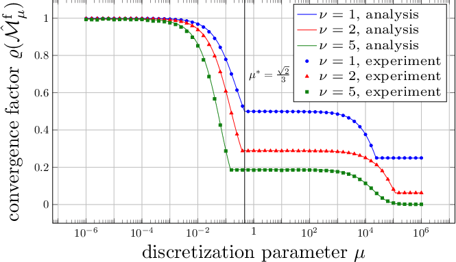
We plot as solid lines in the Figures 3a–3b the theoretical convergence factors $\varrho(\hat{\mathcal{M}}_{\mu}^{\mathrm{s}})$ as functions of the discretization parameter $\mu=\tau_{L}h_{L}^{-2}\in[10^{-6},10^{6}]$ for different polynomial degrees $p_{t}\in\left\{0,1\right\}$ , and different number of smoothing steps $\nu_{1}=\nu_{2}=\nu\in\{1,2,5\}$ . We observe that the theoretical convergence factors are always bounded by $\varrho(\hat{\mathcal{M}}_{\mu}^{\mathrm{s}})\leq\frac{1}{2}$ . For the case when semi coarsening in time is applied we see that the two-grid cycle converges for any discretization parameter $\mu$ . We also see for polynomial degree $p_{t}=1$ that the theoretical convergence factors are much smaller than the theoretical convergence factors for the lowest order case $p_{t}=0$ .

We also plot in Figures 3a–3b using dots, triangles and squares the numerically measured convergence factors for solving the equation

\mathcal{L}_{\tau_{L},h_{L}}\bm{u}=\bm{f}

with the two-grid cycle when semi coarsening in time is applied. For the numerical test we use a zero right hand side, i.e. $\bm{f}=\mathbf{0}$ and a random initial vector $\bm{u}^{0}$ with values between zero and one. The convergence factor of the two-grid cycle is measured by

\displaystyle\max_{k=1,\ldots,N_{\mathrm{iter}}}\frac{{\left\lVert{\bm{r}^{k+1}}\right\rVert}_{2}}{{\left\lVert{\bm{r}^{k}}\right\rVert}_{2}},\quad\text{with }\bm{r}^{k}:=\bm{f}-\mathcal{L}_{\tau_{L},h_{L}}\bm{u}^{k},

where $N_{\mathrm{iter}}\in\mathbb{N}$ , $N_{\mathrm{iter}}\leq 250$ is the number of two-grid iterations used until we have reached a given relative error reduction of $\varepsilon_{\mathrm{MG}}=10^{-140}$ . We observe that the numerical results agree very well with the theoretical results, even though the local Fourier mode analysis is not rigorous for the numerical simulation that does not use periodic boundary conditions.

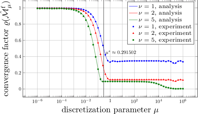
In Figures 4a–4b we plot the theoretical convergence factors $\varrho(\hat{\mathcal{M}}_{\mu}^{\mathrm{s}})$ for the two-grid cycle $\mathcal{M}_{\tau_{L},h_{L}}^{\mathrm{f}}$ with full space-time coarsening as function of the discretization parameter $\mu\in[10^{-6},10^{6}]$ for different polynomial degrees $p_{t}\in\{0,1\}$ . We observe that the theoretical convergence factors are bounded by $\varrho(\hat{\mathcal{M}}_{\mu}^{\mathrm{f}})\leq\frac{1}{2}$ if the discretization parameter $\mu$ is large enough, i.e. for $\mu\geq\mu^{\ast}$ . In Remark 23 we already computed these critical values $\mu^{\ast}$ for several polynomial degrees $p_{t}$ . As before we compared the theoretical results with the numerical results when full space-time coarsening is applied. In Figures 4a–4b the measured numerical convergence factors are plotted as dots, triangles and squares. We see that the theoretical results agree very well with the numerical results.

Overall we conclude that the two-grid cycle always converges to the exact solution of the linear system (3) when semi coarsening in time is applied. Furthermore, if the discretization parameter $\mu$ is large enough, we can also apply full space-time coarsening, which leads to a smaller coarse problem compared to the semi coarsening case.

Remark 36.

For the two-grid analysis above we used for the block Jacobi smoother

(18)

\displaystyle\mathcal{S}_{\tau_{L},h_{L}}^{\nu}=\left[I-\omega_{t}(D_{\tau_{L},h_{L}})^{-1}\mathcal{L}_{\tau_{L},h_{L}}\right]^{\nu}

the exact inverse of the diagonal matrix $D_{\tau_{L},h_{L}}=\mathrm{diag}\left\{A_{\tau_{L},h_{L}}\right\}_{n=1}^{N_{L_{t}}}$ . In practice, it is more efficient to use an approximation $\widetilde{D}_{\tau_{L},h_{L}}^{-1}$ by applying one multigrid iteration in space for the blocks $A_{\tau_{L},h_{L}}$ , see also [34], where such an approximate block Jacobi method is used directly to precondition GMRES. Hence the smoother (18) changes to

(19)

\displaystyle\overline{\mathcal{S}}_{\tau_{L},h_{L}}^{\nu}:=\left[I-\omega_{t}\left(I-\mathcal{M}_{\tau_{L},h_{L}}\right)(D_{\tau_{L},h_{L}})^{-1}\mathcal{L}_{\tau_{L},h_{L}}\right]^{\nu},

with the matrix $\mathcal{M}_{\tau_{L},h_{L}}:=\mathrm{diag}\left\{\mathcal{M}_{\tau_{L},h_{L}}^{x}\right\}_{n=1}^{N_{L_{t}}}$ , where $\mathcal{M}_{\tau_{L},h_{L}}^{x}$ is the iteration matrix of the multigrid scheme for the matrix $A_{\tau_{L},h_{L}}$ . In the case that the iteration matrix $\mathcal{M}_{\tau_{L},h_{L}}^{x}$ is given by a two-grid cycle, we further obtain the representation

\displaystyle\mathcal{M}_{\tau_{L},h_{L}}^{x}=\mathcal{S}_{\tau_{L},h_{L}}^{x,\nu_{2}^{x}}\left[I-\overline{\mathcal{P}}_{x}^{L_{x}}A_{\tau_{L},2h_{L}}^{-1}\overline{\mathcal{R}}_{x}^{L_{x}}A_{\tau_{L},h_{L}}\right]\mathcal{S}_{\tau_{L},h_{L}}^{x,\nu_{1}^{x}},

with a damped Jacobi smoother in space

\displaystyle\mathcal{S}_{\tau_{L},h_{L}}^{x,\nu^{x}}:=\left[I-\omega_{x}\left(D_{\tau_{L},h_{L}}^{x}\right)^{-1}A_{\tau_{L},h_{L}}\right]^{\nu^{x}},\quad D_{\tau_{L},h_{L}}^{x}:=\mathrm{diag}\big\{\frac{2h}{3}K_{\tau_{L}}+\frac{2}{h}M_{\tau_{L}}\big\}_{r=1}^{N_{L_{x}}}

and the restriction and prolongation operators

\displaystyle\overline{\mathcal{R}}_{x}^{L_{x}}:=\mathcal{R}_{x}^{L_{x}}\otimes I_{N_{t}}\quad\text{and}\quad\overline{\mathcal{P}}_{x}^{L_{x}}:=\mathcal{P}_{x}^{L_{x}}\otimes I_{N_{t}}.

With the different smoother (19) we also have to analyze the two different two-grid iteration matrices

(20)		$\displaystyle\overline{\mathcal{M}}_{\tau_{L},h_{L}}^{\mathrm{s}}$	$\displaystyle:=\overline{\mathcal{S}}_{\tau_{L},h_{L}}^{\nu_{2}}\left[I-\mathcal{P}_{\mathrm{s}}^{L_{x},L_{t}}\left(\mathcal{L}_{2\tau_{L},h_{L}}\right)^{-1}\mathcal{R}_{\mathrm{s}}^{L_{x},L_{t}}\mathcal{L}_{\tau_{L},h_{L}}\right]\overline{\mathcal{S}}_{\tau_{L},h_{L}}^{\nu_{1}},$
(21)		$\displaystyle\overline{\mathcal{M}}_{\tau_{L},h_{L}}^{\mathrm{f}}$	$\displaystyle:=\overline{\mathcal{S}}_{\tau_{L},h_{L}}^{\nu_{2}}\left[I-\mathcal{P}_{\mathrm{f}}^{L_{x},L_{t}}\left(\mathcal{L}_{2\tau_{L},2h_{L}}\right)^{-1}\mathcal{R}_{\mathrm{f}}^{L_{x},L_{t}}\mathcal{L}_{\tau_{L},h_{L}}\right]\overline{\mathcal{S}}_{\tau_{L},h_{L}}^{\nu_{1}}.$

Hence it remains to analyze the mapping property of the operator $\mathcal{M}_{\tau_{L},h_{L}}$ on the space of harmonics $\mathcal{E}_{L_{x},L_{t}}(\theta_{x},\theta_{t})$ . By several computations we find under the assumptions of periodic boundary conditions (6) that

\displaystyle\mathcal{M}_{\tau_{L},h_{L}}:\mathcal{E}_{L_{x},L_{t}}(\theta_{x},\theta_{t})\rightarrow\mathcal{E}_{L_{x},L_{t}}(\theta_{x},\theta_{t})

with the mapping

(22)

\displaystyle\begin{pmatrix}U_{1}\\ U_{2}\\ U_{3}\\ U_{4}\end{pmatrix}\mapsto\begin{pmatrix}\widetilde{M}_{\tau_{L},h_{L}}(\theta_{x})&0\\ 0&\widetilde{M}_{\tau_{L},h_{L}}(\theta_{x})\end{pmatrix}\begin{pmatrix}U_{1}\\ U_{2}\\ U_{3}\\ U_{4}\end{pmatrix},

and the iteration matrix

	$\displaystyle\widetilde{M}_{\tau_{L},h_{L}}(\theta_{x})$	$\displaystyle:=\widetilde{\mathcal{S}}_{\tau_{L},h_{L}}^{x,\nu_{1}^{x}}(\theta_{x})\mathcal{K}_{\tau_{L},h_{L}}^{x}(\theta_{x})\widetilde{\mathcal{S}}_{\tau_{L},h_{L}}^{x,\nu_{2}^{x}}(\theta_{x})\in\mathbb{C}^{2N_{t}\times 2N_{t}},$
	$\displaystyle\mathcal{K}_{\tau_{L},h_{L}}^{x}(\theta_{x},\theta_{t})$	$\displaystyle:=I_{2N_{t}}-\widetilde{\mathcal{P}}_{x}(\theta_{x})\widetilde{A}_{\tau_{L},2h_{L}}^{-1}(2\theta_{x})\widetilde{\mathcal{R}}_{x}(\theta_{x})\widetilde{A}_{\tau_{L},h_{L}}(\theta_{x})\in\mathbb{C}^{2N_{t}\times 2N_{t}},$

with the matrices

	$\displaystyle\widetilde{A}_{\tau_{L},h_{L}}(\theta_{x})$	$\displaystyle:=\begin{pmatrix}\hat{A}_{\tau_{L},h_{L}}(\theta_{x})&0\\ 0&\hat{A}_{\tau_{L},h_{L}}(\gamma(\theta_{x}))\end{pmatrix}\in\mathbb{C}^{2N_{t}\times 2N_{t}},$
	$\displaystyle\widetilde{A}_{\tau_{L},2h_{L}}^{-1}(2\theta_{x})$	$\displaystyle:=\left(\hat{A}_{\tau_{L},2h_{L}}(2\theta_{x})\right)^{-1}\in\mathbb{C}^{N_{t}\times N_{t}},$
	$\displaystyle\widetilde{\mathcal{S}}_{\tau_{L},h_{L}}^{x,\nu^{x}}(\theta_{x})$	$\displaystyle:=\begin{pmatrix}\left(\hat{\mathcal{S}}_{\tau_{L},h_{L}}(\omega_{x},\theta_{x})\right)^{\nu^{x}}&0\\ 0&\left(\hat{\mathcal{S}}_{\tau_{L},h_{L}}(\omega_{x},\gamma(\theta_{x}))\right)^{\nu^{x}}\end{pmatrix}\in\mathbb{C}^{2N_{t}\times 2N_{t}},$
	$\displaystyle\widetilde{\mathcal{R}}_{x}(\theta_{x})$	$\displaystyle:=\begin{pmatrix}\hat{\mathcal{R}}_{x}(\theta_{x})I_{N_{t}}&\hat{\mathcal{R}}_{x}(\gamma(\theta_{x}))I_{N_{t}}\end{pmatrix}\in\mathbb{C}^{2N_{t}\times N_{t}},$
	$\displaystyle\widetilde{\mathcal{P}}_{x}(\theta_{x})$	$\displaystyle:=\begin{pmatrix}\hat{\mathcal{P}}_{x}(\theta_{x})I_{N_{t}}\\ \hat{\mathcal{P}}_{x}(\gamma(\theta_{x}))I_{N_{t}}\end{pmatrix}\in\mathbb{C}^{N_{t}\times 2N_{t}},$

and the Fourier symbols

	$\displaystyle\hat{A}_{\tau_{L},h_{L}}(\theta_{x})$	$\displaystyle:=\frac{h_{L}}{3}\left(2+\cos(\theta_{x})\right)K_{\tau_{L}}+\frac{2}{h_{L}}\left(1-\cos(\theta_{x})\right)M_{\tau_{L}}\in\mathbb{C}^{N_{t}\times N_{t}},$
	$\displaystyle\hat{\mathcal{S}}_{\tau_{L},h_{L}}(\omega_{x},\theta_{x})$	$\displaystyle:=I_{N_{t}}-\omega_{x}\left(\frac{2h_{L}}{3}K_{\tau_{L}}+\frac{2}{h_{L}}M_{\tau_{L}}\right)^{-1}\hat{A}_{\tau_{L},h_{L}}(\theta_{x})\in\mathbb{C}^{N_{t}\times N_{t}}.$

Hence we can analyze the modified two-grid iteration matrices (20) by taking the additional approximation with the mapping (22) into account. For the smoothing steps $\nu_{1}^{x}=\nu_{2}^{x}=2$ and the damping parameter $\omega_{x}=\frac{2}{3}$ for the spatial multigrid component, the theoretical convergence factors with semi coarsening in time are plotted in Figures 5a–5b for the discretization parameter $\mu\in[10^{-6},10^{6}]$ with respect to the polynomial degrees $p_{t}\in\{0,1\}$ . We observe that the theoretical convergence factors are always bounded by $\varrho(\overline{\mathcal{M}}_{\mu}^{\mathrm{s}})\leq\frac{1}{2}$ . We also notice that the theoretical convergence factors are a little bit larger for small discretization parameters $\mu$ , compared to the case when the exact inverse of the diagonal matrix $D_{\tau_{L},h_{L}}$ is used. The numerical factors are plotted as dots, triangles and squares in Figures 5a–5b. We observe that the theoretical convergence factors coincide with the numerical results.

In Figures 6a–6b the convergence of the two-grid cycle for the full space-time coarsening case is studied. Here we see that the computed convergence factors are very close to the results which we obtained for the case when the exact inverse of the diagonal matrix $D_{\tau_{L},h_{L}}$ is used.

4 Numerical examples

We present now numerical results for the multigrid version of our algorithm, for which we analyzed the two-grid cycle in Section 3.2. Following our two-grid analysis, we also apply full space-time coarsening only if $\mu_{L}\geq\mu^{\ast}$ in the multigrid version. If $\mu_{L}<\mu^{\ast}$ , we only apply semi coarsening in time. In that case, we will have for the next coarser level $\mu_{L-1}=2\tau_{L}h_{L}^{-2}=2\mu_{L}$ . This implies that the discretization parameter $\mu_{L-1}$ gets larger when semi coarsening in time is used. Hence, if $\mu_{L-k}\geq\mu^{\ast}$ for $k<L$ we can apply full space-time coarsening to reduce the computational costs. If full space-time coarsening is applied, we have $\mu_{L-1}=2\tau_{L}\left(2h_{L}\right)^{-2}=\frac{1}{2}\mu_{L}$ , which results in a smaller discretization parameter $\mu_{L-1}$ . We therefore will combine semi coarsening in time or full space-time coarsening in the right way to get to the next coarser space-time level. For different discretization parameters $\mu=c\mu^{\ast}$ , $c\in\{1,10\}$ , this coarsening strategy is shown in Figure 7 for 8 time and 4 space levels. The restriction and prolongation operators for the space-time multigrid scheme are then defined by the given coarsening strategy.

We now show examples to illustrate the performance of our new space-time multigrid method.

Example 37 (Multigrid iterations).

In this example we consider the spatial domain $\Omega=(0,1)^{3}$ and the simulation interval $(0,T)$ with $T=1$ . The initial decomposition for the spatial domain $\Omega$ is given by $12$ tetrahedra. We use several uniform refinement levels to study the convergence behavior of the space-time multigrid solver with respect to the space-discretization. For the coarsest time level we use one time step, i.e. $\tau_{0}=1$ . For the space discretization we use P1 conforming finite elements and for the time discretization we use piecewise linear discontinuous ansatz functions, i.e. $p_{t}=1$ . To test the performance of the space-time multigrid method we use a zero right hand side, i.e. $\bm{f}=\mathbf{0}$ and as an initial guess $\bm{u}^{0}$ we use a random vector with values between zero and one. For the space-time multigrid solver we use $\nu_{1}=\nu_{2}=2$ , $\omega_{t}=\frac{1}{2}$ , $\gamma=1$ . We apply for each block $A_{\tau_{L},h_{L}}$ one geometric multigrid V-cycle to approximate the inverse of the diagonal matrix $D_{\tau_{L},h_{L}}$ . For this multigrid cycle we use $\nu_{1}^{x}=\nu_{2}^{x}=2$ , $\omega_{x}=\frac{2}{3}$ , $\gamma_{x}=1$ . For the smoother we use a damped block Jacobi smoother. We apply the space-time multigrid solver until we have reached a given relative error reduction of $\varepsilon_{\mathrm{MG}}=10^{-8}$ . In Table 1, the iteration numbers for several space and time levels are given. We observe that the iteration numbers stay bounded independently of the mesh size $h_{L_{x}}$ , the time step size $\tau_{L_{t}}$ and the number of time steps $N_{L_{t}}=2^{L_{t}}$ .

				time levels
		$0$	$1$	$2$	$3$	$4$	$5$	$6$	$7$	$8$	$9$	$10$	$11$	$12$	$13$	$14$
space levels	$0$	$1$	$7$	$7$	$7$	$7$	$7$	$7$	$7$	$8$	$8$	$9$	$9$	$9$	$9$	$9$
	$1$	$1$	$7$	$7$	$7$	$7$	$7$	$7$	$7$	$8$	$8$	$9$	$9$	$9$	$9$	$9$
	$2$	$1$	$7$	$7$	$7$	$7$	$7$	$8$	$7$	$8$	$8$	$9$	$9$	$9$	$9$	$9$
	$3$	$1$	$7$	$7$	$7$	$7$	$8$	$8$	$8$	$8$	$8$	$9$	$9$	$9$	$9$	$9$
	$4$	$1$	$7$	$7$	$7$	$8$	$8$	$8$	$8$	$8$	$8$	$8$	$9$	$9$	$9$	$9$
	$5$	$1$	$7$	$7$	$7$	$7$	$7$	$8$	$8$	$8$	$8$	$8$	$9$	$9$	$9$	$9$

Table 1: Multigrid iterations for Example 37.

Example 38 (High order time discretizations).

In this example we study the convergence of the space-time multigrid method for different polynomial degrees $p_{t}$ , which are used for the underlying time discretization. To do so, we consider the spatial domain $\Omega=(0,1)^{2}$ and the simulation interval $(0,T)$ with $T=1024$ . For the space-time discretization we use tensor product space-time elements with piecewise linear continuous ansatz functions in space, and for the discretization in time we use a fixed time step size $\tau=1$ . For the initial triangulation of the spatial domain $\Omega$ we consider $4$ triangles, which are refined uniformly several times. For the space-time multigrid approach we use the same parameters as in Example 37. We solve the linear system (4) with zero right hand side, i.e. $\bm{f}=\mathbf{0}$ and for the initial vector $\bm{u}^{0}$ we use a random vector with values between zero and one. We apply the space-time multigrid solver until we have reached a relative error reduction of $\varepsilon_{\mathrm{MG}}=10^{-8}$ . In Table 2 the iteration numbers for different polynomial degrees $p_{t}$ and different space levels are given. We observe that the iteration numbers are bounded, independently of the ansatz functions for the time discretization.

		polynomial degree $p_{t}$
		$0$	$1$	$2$	$3$	$4$	$5$	$10$	$15$	$20$	$25$	$30$	$35$	$40$	$45$
space levels	$0$	$7$	$7$	$6$	$6$	$6$	$6$	$5$	$5$	$4$	$4$	$4$	$4$	$5$	$5$
	$1$	$7$	$7$	$7$	$7$	$7$	$7$	$7$	$7$	$7$	$7$	$7$	$7$	$7$	$7$
	$2$	$7$	$7$	$7$	$7$	$7$	$7$	$7$	$7$	$7$	$7$	$7$	$7$	$7$	$7$
	$3$	$7$	$7$	$7$	$7$	$7$	$7$	$7$	$7$	$7$	$7$	$7$	$7$	$7$	$7$
	$4$	$7$	$7$	$7$	$7$	$7$	$7$	$7$	$7$	$7$	$7$	$7$	$7$	$7$	$7$
	$5$	$7$	$7$	$7$	$7$	$7$	$7$	$7$	$7$	$7$	$7$	$7$	$7$	$7$	$7$
	$6$	$7$	$7$	$7$	$7$	$7$	$7$	$7$	$7$	$7$	$7$	$7$	$7$	$7$	$7$
	$7$	$7$	$7$	$7$	$7$	$7$	$7$	$7$	$7$	$7$	$7$	$7$	$7$	$7$	$7$

Table 2: Multigrid iterations with respect to the polynomial degree

p_{t}

5 Parallelization

One big advantage of our new space-time multigrid method is that it can be parallelized also in the time direction, i.e. the damped block Jacobi smoother can be executed in parallel in time. For each time step we have to apply one multigrid cycle in space to approximate the inverse of the diagonal matrix $D_{\tau_{L},h_{L}}$ . The application of this space multigrid cycle can also be done in parallel, where one may use parallel packages like in [6, 5, 24]. Hence the problem (4) can be fully parallelized in space and time, see Figure 8.

The next example shows the excellent weak and strong scaling properties of our new space-time multigrid method.

Example 39 (Parallel computations).

In this example we consider the spatial domain $\Omega=(0,1)^{3}$ , which is decomposed into $49\;152$ tetrahedra. For the discretization in space we use P1 conforming finite elements and for the time discretization we use polynomials of order $p_{t}=3$ and a fixed time step size $\tau=10^{-1}$ . For the multigrid solver in space we use the best possible settings such that we obtain the smallest computational times when we apply the usual forward substitution. In particular we use a damped Gauß-Seidel smoother with the damping parameter $\omega_{x}=1.285$ and we apply one pre- and one post-smoothing step, i.e. $\nu_{1}^{x}=\nu_{2}^{x}=1$ . We also tune the multigrid parameters with respect to time, such that we also obtain the best possible computational times for the presented space-time multigrid solver. Here we use $\nu_{1}=\nu_{2}=1$ smoothing steps and since $\mu=\tau h^{-2}$ is large enough we use for the damping parameter $\omega_{t}=1$ , see also Remark 24. Of course we could also use the assymptotic optimal damping parameter $\omega_{t}^{\ast}=\frac{1}{2}$ which would lead to slightly more multigrid iterations for this case.

To show the parallel performance, we first study the weak scaling behavior of the new multigrid method. We use a fixed number of time steps per core, i.e. $2$ time steps for each core, and we increase the number of cores when we increase the number of time steps. Hence the computational cost for one space-time multigrid cycle stays almost the same for each core. Only the cost for the communication grows, since the space-time hierarchy gets bigger, when we increase the number of time steps. In Table 9a, we give timings for solving the linear system (4) for a different number of time steps. We see that the multigrid iterations stay bounded, if we increase the problem size and that the computational costs stay completely constant if we increase the number of cores. We also compare the presented space-time multigrid solver with the usual forward substitution. For this we apply for each time step the space multigrid solver with the best possible settings from above. We run the space multigrid solver until we obtain the same relative error tolerance as for the space-time multigrid method. In Table 9a the timings for the forward substitution are compared with the parallel space-time multigrid solver. Here we observe that the space-time multigrid solver is already faster when we use only two cores. Furthermore, when we increase the number of cores we observe that the space-time multigrid approach completely outperforms the forward substitution.

To test the strong scaling behavior, we fix the problem size and use $32\;768$ time steps, which results in a linear system with $979\;238\;912$ unknowns. Then we increase the number of cores, which results in smaller and smaller problems per computing core. In Table 9b the timings are given for different numbers of cores. We see that the computational costs are divided by a factor very close to two, if we double the number of cores. All the parallel computations of this example were performed on the Lemanicus BlueGene/Q Supercomputer in Lausanne, Switzerland, and for one, two and four cores, the computational times needed were too large to run, since Lemanicus has a maximum wall clock time restriction of 24 hours.

cores	time steps	dof	iter	time	fwd. sub.
$1$	$2$	$59\;768$	$7$	$29.3$	$21.2$
$2$	$4$	$119\;536$	$7$	$29.6$	$44.0$
$4$	$8$	$239\;072$	$7$	$29.6$	$87.7$
$8$	$16$	$478\;144$	$7$	$29.7$	$176.7$
$16$	$32$	$956\;288$	$7$	$29.6$	$351.7$
$32$	$64$	$1\;912\;576$	$7$	$29.7$	$703.8$
$64$	$128$	$3\;825\;152$	$7$	$29.7$	$1\;408.3$
$128$	$256$	$7\;650\;304$	$7$	$29.7$	$2\;819.8$
$256$	$512$	$15\;300\;608$	$7$	$29.8$	$5\;662.7$
$512$	$1\;024$	$30\;601\;216$	$7$	$29.7$	$11\;278.4$
$1\;024$	$2\;048$	$61\;202\;432$	$7$	$29.8$	$22\;560.3$
$2\;048$	$4\;096$	$122\;404\;864$	$7$	$29.7$	$45\;111.3$
$4\;096$	$8\;192$	$244\;809\;728$	$7$	$29.7$	$87\;239.8$
$8\;192$	$16\;384$	$489\;619\;456$	$7$	$29.8$	$174\;283.5$
$16\;384$	$32\;768$	$979\;238\;912$	$7$	$29.7$	$348\;324.0$

(a) Weak scaling results.

cores	time steps	dof	iter	time
$1$	$32\;768$	$979\;238\;912$	$7$	$-$
$2$	$32\;768$	$979\;238\;912$	$7$	$-$
$4$	$32\;768$	$979\;238\;912$	$7$	$-$
$8$	$32\;768$	$979\;238\;912$	$7$	$60\;232.5$
$16$	$32\;768$	$979\;238\;912$	$7$	$30\;239.5$
$32$	$32\;768$	$979\;238\;912$	$7$	$15\;136.2$
$64$	$32\;768$	$979\;238\;912$	$7$	$7\;590.0$
$128$	$32\;768$	$979\;238\;912$	$7$	$3\;805.2$
$256$	$32\;768$	$979\;238\;912$	$7$	$1\;906.8$
$512$	$32\;768$	$979\;238\;912$	$7$	$951.8$
$1\;024$	$32\;768$	$979\;238\;912$	$7$	$473.4$
$2\;048$	$32\;768$	$979\;238\;912$	$7$	$238.2$
$4\;096$	$32\;768$	$979\;238\;912$	$7$	$119.0$
$8\;192$	$32\;768$	$979\;238\;912$	$7$	$59.4$
$16\;384$	$32\;768$	$979\;238\;912$	$7$	$29.7$

(b) Strong scaling results.

Fig. 9: Scaling results with solving times in seconds.

6 Conclusions

We presented a new space-time multigrid method for the heat equation, and used local Fourier mode analysis to give precise asymptotic convergence and parameter estimates for the two-grid cycle. We showed that this asymptotic analysis predicts very well the performance of the new algorithm, and our parallel implementation gave excellent weak and strong scaling results for a large number of processors.

This new space-time multigrid algorithm can not only be used for the heat equation, it is applicable to general parabolic problems. It has successfully been applied to the time dependent Stokes equations, where one obtains similar speed up results as for the heat equation. Furthermore, this technique has been applied successfully to parabolic control problems, but the analysis and the results will appear elsewhere.

Acknowledgments

The financial support for CADMOS and the Blue Gene/Q system is provided by the Canton of Geneva, Canton of Vaud, Hans Wilsdorf Foundation, Louis-Jeantet Foundation, University of Geneva, University of Lausanne, and Ecole Polytechnique Fédérale de Lausanne.

References

[1] G. Bal. On the convergence and the stability of the parareal algorithm to solve partial differential equations. Lect. Notes Comput. Sci. Eng., Springer, Berlin, 40:425–432, 2005.
[2] D. Bennequin, M. J. Gander, and L. Halpern. A homographic best approximation problem with application to optimized Schwarz waveform relaxation. Mathematics of Computation, 78(265):185–223, 2009.
[3] S. Börm and R. Hiptmair. Analysis of tensor product multigrid. Numer. Algorithms, 26:219–234, 2001.
[4] M. Emmett and M. L. Minion. Toward an efficient parallel in time method for partial differential equations. Comm. App. Math. and Comp. Sci, 7(1):105–132, 2012.
[5] R. Falgout, J. Jones, and U. Yang. The design and implementation of hypre, a library of parallel high performance preconditioners. Lect. Notes Comput. Sci. Eng., 51:267–294, 2006.
[6] R. Falgout and U. Yang. hypre: A Library of High Performance Preconditioners. Proceedings of the International Conference on Computational Science-Part III, pages 632–641, 2002.
[7] M. J. Gander. A waveform relaxation algorithm with overlapping splitting for reaction diffusion equations. Numerical Linear Algebra with Applications, 6:125–145, 1998.
[8] M. J. Gander. 50 years of time parallel time integration. In Multiple Shooting and Time Domain Decomposition Methods. Springer Verlag, 2014.
[9] M. J. Gander and E. Hairer. Nonlinear convergence analysis for the parareal algorithm. In O. B. Widlund and D. E. Keyes, editors, Domain Decomposition Methods in Science and Engineering XVII, volume 60 of Lecture Notes in Computational Science and Engineering, pages 45–56. Springer, 2008.
[10] M. J. Gander and L. Halpern. Absorbing boundary conditions for the wave equation and parallel computing. Math. of Comp., 74(249):153–176, 2004.
[11] M. J. Gander and L. Halpern. Optimized Schwarz waveform relaxation methods for advection reaction diffusion problems. SIAM J. Numer. Anal., 45(2):666–697, 2007.
[12] M. J. Gander, L. Halpern, and F. Nataf. Optimal convergence for overlapping and non-overlapping Schwarz waveform relaxation. In C.-H. Lai, P. Bjørstad, M. Cross, and O. Widlund, editors, Eleventh international Conference of Domain Decomposition Methods. ddm.org, 1999.
[13] M. J. Gander, L. Halpern, and F. Nataf. Optimal Schwarz waveform relaxation for the one dimensional wave equation. SIAM Journal of Numerical Analysis, 41(5):1643–1681, 2003.
[14] M. J. Gander, Y.-L. Jiang, and R.-J. Li. Parareal Schwarz waveform relaxation methods. In O. B. Widlund and D. E. Keyes, editors, Domain Decomposition Methods in Science and Engineering XX, volume 60 of Lecture Notes in Computational Science and Engineering, pages 45–56, 2013.
[15] M. J. Gander, F. Kwok, and B. Mandal. Dirichlet-Neumann and Neumann-Neumann waveform relaxation algorithms for parabolic problems. 2014. submitted.
[16] M. J. Gander and M. Neumüller. Analysis of a time multigrid algorithm for DG-discretizations in time. SIAM J. Num. Anal., 2014. submitted.
[17] M. J. Gander and A. M. Stuart. Space-time continuous analysis of waveform relaxation for the heat equation. SIAM J. Sci. Comput., 19(6):2014–2031, 1998.
[18] M. J. Gander and S. Vandewalle. Analysis of the parareal time-parallel time-integration method. SIAM J. Sci. Comput., 29:556–578, 2007.
[19] E. Giladi and H. B. Keller. Space time domain decomposition for parabolic problems. Numerische Mathematik, 93(2):279–313, 2002.
[20] W. Hackbusch. Parabolic multigrid methods. Computing methods in applied sciences and engineering, VI, pages 189–197, 1984.
[21] W. Hackbusch. Multi-Grid Methods and Applications. Springer, Berlin, 1985.
[22] E. Hairer, S. P. Nørsett, and G. Wanner. Solving ordinary differential equations. I. Nonstiff problems. Springer Series in Computational Mathematics, 8. Springer-Verlag, Berlin, 1993.
[23] E. Hairer and G. Wanner. Solving ordinary differential equations. II. Stiff and differential-algebraic problems. Springer Series in Computational Mathematics, 14. Springer-Verlag, Berlin, 2010.
[24] I. Heppner, M. Lampe, A. Nägel, S. Reiter, M. Rupp, A. Vogel, and G. Wittum. Software Framework ug4: Parallel Multigrid on the Hermit Supercomputer. High Performance Computing in Science and Engineering, 12:435–449, 2013.
[25] G. Horton. The time-parallel multigrid method. Comm. Appl. Numer. Methods, 8:585–595, 1992.
[26] G. Horton and S. Vandewalle. A space-time multigrid method for parabolic partial differential equations. SIAM J. Sci. Comput., 16:848–864, 1995.
[27] G. Horton, S. Vandewalle, and P. Worley. An algorithm with polylog parallel complexity for solving parabolic partial differential equations. SIAM J. Sci. Comput., 16:531–541, 1995.
[28] F. Kwok. Neumann-Neumann waveform relaxation for the time-dependent heat equation. In Domain decomposition methods in science and engineering, DD21. Springer, 2014.
[29] J.-L. Lions, Y. Maday, and G. Turinici. A parareal in time discretization of PDEs. C.R. Acad. Sci. Paris, Serie I, 332:661–668, 2001.
[30] C. Lubich and A. Ostermann. Multigrid dynamic iteration for parabolic equations. BIT, 27:216–234, 1987.
[31] Y. Maday. A parareal in time procedure for the control of partial differential equations. C. R. Math. Acad. Sci. Paris, 335:387–392, 2002.
[32] Y. Maday and G. Turinici. The parareal in time iterative solver: a further direction to parallel implementation. Lect. Notes Comput. Sci. Eng., Springer, Berlin, 40:441–448, 2005.
[33] B. Mandal. A time-dependent Dirichlet-Neumann method for the heat equation. In Domain decomposition methods in science and engineering, DD21. Springer, 2014.
[34] E. G. McDonald and A. J. Wathen. A simple proposal for parallel computing over time of an evolutionary process with implicit time stepping. preprint, 2014.
[35] R. Speck, D. Ruprecht, M. Emmett, M. Minion, M. Bolten, and R. Krause. A multi-level spectral deferred correction method. arXiv preprint arXiv:1307.1312, 2013.
[36] R. Speck, D. Ruprecht, R. Krause, M. Emmett, M. Minion, M. Winkel, and P. Gibbon. A massively space-time parallel n-body solver. In Proceedings of the International Conference on High Performance Computing, Networking, Storage and Analysis, page 92. IEEE Computer Society Press, 2012.
[37] G. Staff and E. Rønquist. Stability of the parareal algorithm. Lect. Notes Comput. Sci. Eng., Springer, Berlin, 40:449–456, 2005.
[38] V. Thomée. Galerkin Finite Element Methods for Parabolic Problems. Springer, New York, 2006.
[39] U. Trottenberg, C. W. Oosterlee, and A. Schüller. Multigrid. Academic Press, Inc., San Diego, 2001.
[40] S. Vandewalle and E. de Velde. Space-time concurrent multigrid waveform relaxation. Ann. Numer. Math., 1:347–360, 1994.
[41] S. Vandewalle and R. Piessens. Efficient parallel algorithms for solving initial-boundary value and time-periodic parabolic partial differential equations. SIAM J. Sci. Statist. Comput., 13:1330–1346, 1992.
[42] P. Vassilevski. Multilevel block factorization preconditioners. Springer, New York, 2008.
[43] T. Weinzierl and T. Köppl. A geometric space-time multigrid algorithm for the heat equation. Numer. Math. Theory Methods Appl., 5:110–130, 2012.
[44] P. Wesseling. An Introduction to Multigrid Methods. John Wiley & Sons Ltd., 1992. Corrected Reprint. Philadelphia: R.T. Edwards, Inc., 2004.

Analysis of a New Space-Time Parallel Multigrid Algorithm for Parabolic Problems

Abstract

keywords

AMS

1 Introduction

2 Multigrid method

Theorem 1 (Discrete Fourier transform).

Definition 2 (Fourier modes, Fourier frequencies).

Definition 3 (Fourier space).

Definition 4 (Space of harmonics).

Lemma 5.

Lemma 6.

Lemma 7.

Lemma 8.

Lemma 9.

Lemma 10.

3 Local Fourier mode analysis

3.1 Smoothing analysis

Lemma 11.

Proof.

Definition 12 (Fourier space).

Lemma 13 (Shifting equality).

Proof.

Lemma 14 (Fourier symbol of ℒτL,hL\mathcal{L}_{\tau_{L},h_{L}}).

Proof.

Lemma 15 (Mapping property of 𝒮τL,hLν\mathcal{S}_{\tau_{L},h_{L}}^{\nu}).

Proof.

Definition 16 (High and low frequency ranges).

Definition 17 (Asymptotic smoothing factors).

Lemma 18.

Proof.

Lemma 19.

Proof.

Lemma 20 (Asymptotic smoothing factor for semi-coarsening).

Proof.

Lemma 21 (Asymptotic smoothing factor for full space-time coarsening).

Proof.

Lemma 22.

Proof.

Remark 23.

Remark 24.

3.2 Two-grid analysis

Lemma 25.

Proof.

Definition 26 (Space of harmonics).

Lemma 27.

Proof.

Definition 28.

Lemma 29.

Proof.

Lemma 30.

Proof.

Lemma 31.

Proof.

Lemma 32.

Proof.

Theorem 33.

Proof.

Theorem 34.

Proof.

Definition 35 (Asymptotic two-grid convergence factors).

Remark 36.

4 Numerical examples

Example 37 (Multigrid iterations).

Example 38 (High order time discretizations).

5 Parallelization

Example 39 (Parallel computations).

6 Conclusions

Acknowledgments

References

Lemma 14 (Fourier symbol of $\mathcal{L}_{\tau_{L},h_{L}}$ ).

Lemma 15 (Mapping property of $\mathcal{S}_{\tau_{L},h_{L}}^{\nu}$ ).