Modulated escape from a metastable state driven by colored noise
Abstract
Many phenomena in nature are described by excitable systems driven by colored noise. The temporal correlations in the fluctuations hinder an analytical treatment. We here present a general method of reduction to a white-noise system, capturing the color of the noise by effective and time-dependent boundary conditions. We apply the formalism to a model of the excitability of neuronal membranes, the leaky integrate-and-fire neuron model, revealing an analytical expression for the linear response of the system valid up to moderate frequencies. The closed form analytical expression enables the characterization of the response properties of such excitable units and the assessment of oscillations emerging in networks thereof.
pacs
05.40.-a, 05.10.Gg, 87.19.llI Introduction
In his pioneering work Kramers [1] investigated chemical reaction rates by considering the noise-activated escape from a metastable state as a problem of Brownian motion over a barrier. In the overdamped case, this generic setting applies to various phenomena ranging from ion channel gating [2], Josephson junctions [3, 4, 5], tunnel diodes [6], semiconductor lasers [7] to abstract models of cancer growth [8]. These studies assume the noise statistics to have a white spectrum. This idealization simplifies the analytical treatment and is the limit of non-white processes for vanishing correlation time [9]. White noise cannot exist in real systems, which is obvious considering, for example, the voltage fluctuations generated by thermal agitation in a resistor [10, 11]: if fluctuations had a flat spectrum, power dissipation would be infinite. In a non-equilibrium setting a system is driven by an external fluctuating force. The simplest model for such a non-white noise is characterized by a single time constant, representing a more realistic colored-noise model.
The effect of colored noise is relevant in modeling the phase difference in lasers [12], the velocity in turbulence models [13], genetic selection [14] and chemical reactions [15] (for further examples see [16, 17]). Its influence on the escape from a metastable state has been studied theoretically as the stationary mean first passage time (MFPT) of a particle in the Landau potential [18, 15, 19, 20, 21, 22]. Treating colored noise analytically comes along with considerable difficulties, since it adds a dimension to the governing Fokker-Planck equation (FPE) and the common strategy is to reduce the colored-noise problem to an effective white-noise system. Doering et al. [22] and Kłosek and Hagan [23] developed these approaches further by singular perturbation methods and boundary-layer theory, showing that the leading order correction to the static MFPT stems from an appropriate treatment of the boundary conditions of the effective system.
The organization of this work is as follows. In Section II we extend the works by Doering et al. [22] and Kłosek and Hagan [23] to the time-dependent case by a perturbation expansion of the flux operator appearing in the FPE itself. This approach leads to a general method that reduces a first order differential equation driven by additive and fast colored noise to an effective one-dimensional system, allowing the study of time-dependent phenomena and thus revealing the spectral properties of the system. The effective formulation implicitly contains the matching between outer and boundary-layer solutions. The latter appear close to absorbing boundaries and are obtained by a half-range expansion. Our main result is that colored-noise approximations for stationary but more importantly also for dynamic quantities are directly obtained by shifting the location of the boundary conditions in the solutions for the corresponding white-noise system.
In Section III we apply this general result to the particular problem of modeling biological membranes: the leaky integrate-and-fire (LIF) neuron model [24, 25] with exponentially decaying post-synaptic currents can equivalently be described as a first-order differential equation driven by colored noise. Based on the works of Doering et al. [22] and Kłosek and Hagan [23], Brunel et al. [26, 27] calculated the high-frequency limit of its transfer function. Here we complement these works deriving a novel analytical expression for the transfer function valid up to moderate frequencies, which we confirm by direct simulations. While for slow noise, an adiabatic approximation for the transfer function is known [28], this first order correction in the time scale of the noise is a qualitatively new result. In the previous work by Fourcaud and Brunel [27] it was shown that the first order correction vanishes in case of the integrate-and-fire neuron without a leak term, i.e. for the perfect integrator (PIF). For this type of neuron, the marginal statistics of the spike train was characterized for an arbitrary time scale of the noise with weak amplitude [29]. Further extensions to multiple time scales have recently been developed [30]. However, to date the correction to the transfer function of the LIF model is unknown in the biologically relevant regime of moderate frequencies.
The transfer function is at the heart of the contemporary theory of fluctuations in spiking neuronal networks [31, 32] and allows the derivation of analytical expressions for experimentally observable measures, such as pairwise correlations [33] and oscillations in the population activity [34, 35]. In Section IV we show analytically how realistic synaptic filtering affects the power spectrum in a recurrent network of excitatory and inhibitory neurons, a question that has been inaccessible prior to the present work.
II Reduction from colored to white noise
Consider a pair of coupled stochastic differential equations (SDE) with a slow component with time scale , driven by a fast Ornstein-Uhlenbeck process with time scale . In dimensionless time and with relating the two time constants we have
| (1) |
with a unit variance white noise . The setting (1) describes an overdamped Brownian motion of a particle in a possibly time dependent potential , driven by colored noise. The generic problem of escape from such a potential is illustrated in Figure 1A where the particle has to overcome a smooth barrier. The latter can be simplified, assuming an absorbing boundary at the right end of the domain, illustrated in Figure 1B for the quadratic potential . The potential (Figure 1C) is regarded as the archetypal form giving rise to a bistable system and is reviewed in [36] and [37]. The MFTP from one well to the peak of the potential can be calculated by assuming an absorbing boundary at the maximum, formally reducing this case to the one shown in Figure 1B. Note that the MFTP from one well to the other is not directly related to the MFTP to the peak, but rather is twice the MFTP to an absorbing boundary on the separatrix in the two-dimensional domain [38] spanned by and . However, we are here interested in the case where the component crosses a constant threshold value [39].

Initially we revisit the intuitive argument that in the case of fast noise the slow component approximately obeys the one-dimensional SDE . Heuristically this can be viewed as integrating on a time scale . For finite the integral of the autocorrelation of is , identical to the limit of vanishing , where becomes a white noise. We here set out to formally derive an effective diffusion equation for to obtain a formulation in which we can include the absorbing boundaries that are essential to study an escape problem. We consider the FPE [40] corresponding to the two-dimensional system (1)
| (2) |
where denotes the probability density and we introduce the probability flux operator in -direction as . Factoring-off the stationary solution of the fast part of the Fokker-Planck operator, , we observe the change of the differential operator , which transforms (2) to
| (3) |
We refer to as the outer solution, since initially we do not consider the absorbing boundary condition. The strategy is as follows: we show that the terms of first and second order in the small parameter of the perturbation ansatz
| (4) |
cause an effective flux acting on the -marginalized solution that can be expressed as a one-dimensional FPE which is correct up to linear order in . To this end we need to know the first order correction to the marginalized probability flux . Inserting the perturbation ansatz (4) into (3) we have . Noting the property , we see that the lowest order does not imply any further constraints on the -independent solution , which must be consistent with the solution to the one-dimensional Fokker-Planck equation corresponding to the limit of (1). The first and second orders are
| (5) | |||||
With , the general solution for the first order
| (6) |
leaves the freedom to choose a homogeneous (-independent) solution of . To generate the term linear in on the right hand side of the second order in (5), we need a term . The terms constant in require contributions proportional to , because . However, they can be dropped right away since their contribution to vanishes after marginalization. For the same reason the homogeneous solution can be dropped. Collecting all terms which contribute to in orders and higher in , the only relevant part of the second order solution is , which leaves us with
| (7) | ||||
from which we obtain the marginalized flux
| (8) |
We observe that is the flux operator of a one-dimensional system driven by a unit variance white noise and is the marginalization of (7) over . Note that in (7) the higher order terms in appear due to the operator in (3) that couples the and coordinate. Eq. (8) shows that these terms cause an effective flux that only depends on the -marginalized solution . This allows us to obtain the time evolution by applying the continuity equation to the effective flux (8) yielding the effective FPE
| (9) |

Effective FPEs, to first order identical to (9), but also including higher order terms, have been derived earlier [18, 15, 19, 20, 21]. These approaches have been criticized for an untended treatment of the boundary conditions of the effective system [23]. Doering et al. [22] and Kłosek and Hagan [23] used singular perturbation methods and boundary layer theory to show that the correction to the static MFPT stems from colored-noise boundary conditions for the marginalized density of the effective system. Extending this approach to the transient case requires a time-dependent boundary condition for or, equivalently, for , because we assume the one-dimensional problem to be exactly solvable and hence the boundary value of to be known. Without loss of generality, we assume an absorbing boundary at the right end of the domain. Thus trajectories must not enter the domain from above threshold, implying the flux to vanish at for all points with negative velocity in given by . A change of coordinates simplifies the condition to for . The flux and this half range boundary condition are shown in Figure 2A. The resulting boundary layer at requires the transformation of the FPE (3) to the shifted and scaled coordinate , which yields
| (10) | ||||
with and the operator . The boundary condition then takes the form
| (11) |
With the perturbation ansatz we obtain
| (12) |
the solution of which must match the outer solution. The latter varies only weakly on the scale of and therefore a first order Taylor expansion at the boundary yields the matching condition , illustrated in Figure 2B. We note with that the zeroth order vanishes. Inserting (6) into the matching condition, with the instantaneous flux in the white-noise system, the first order takes the form
| (13) |
The vanishing zeroth order implies with (12) for the first order Appendix B of Kłosek and Hagan [23] states the solution of the latter equation satisfying the half-range boundary condition
| (14) |
with given by Riemann’s -function and proportional to the -th Hermite polynomial. We equate (14) to (13) neglecting the latter exponential term which decays on a small length scale, so that the term proportional to fixes the time dependent function and hence the boundary value . This yields the central result of our theory: We have reduced the colored-noise problem (1) to the solution of a one-dimensional FPE (9) with the time-dependent boundary condition
| (15) |
where the time-dependent flux is obtained from the solution of the corresponding white-noise problem. The boundary condition can be understood intuitively: the filtered noise slows down the diffusion at the absorbing boundary with increasing ; the noise spectrum and the velocity of are bounded, so in contrast to the white-noise case, there can be a finite density at the boundary. Its magnitude results from a momentary equilibrium of the escape crossing the boundary and the flow towards it, where the latter is approximated by the flow at threshold in the white noise system. In principle one can obtain colored-noise solutions combining the effective system (9) with the time-dependent colored-noise boundary condition (15), which is explicitly shown in [41]. Here we aim for an even further reduction, recasting this time-dependent boundary condition into a static condition by considering a shift in the threshold
| (16) |
We perform a Taylor expansion of the effective density
| (17) |
using (15) and to show that the density vanishes to order . As a result, to first order in the dynamic boundary condition (15) can be rewritten as a perfectly absorbing (white-noise) boundary at shifted (16). For the particular problem of the stationary MFPT this was already found by Kłosek and Hagan [23] and Fourcaud and Brunel [27] as a corollary deduced from the steady state density rather than as the result of a generic reduction of a colored- to a white-noise problem. It remained unclear from these earlier works, whether and how it is possible to apply the effective FPE to time-dependent problems. We show above that the effective FPE (9) that directly follows from a perturbation expansion of the flux operator can be re-summed to an effective operator acting on a one-dimensional density. This, together with the effective boundary condition (15) or (16), is the crucial step to reduce the time-dependent problem driven by colored noise to an effective time-dependent white-noise problem, rendering the transient properties of the system accessible to an analytical treatment.
After escape certain physical systems reset the dynamic variable to a value , while leaving the noise variable unchanged. Note that the noise density at reset therefore does not follow the marginalized density shown in Figure 2. Instead, due to the fire and reset rule, it is biased to strictly positive noise values and in the limit of weak noise its approximate form was calculated for the PIF neuron [29]. In the presence of such a reset our calculation (see Appendix A) yields the additional boundary condition , which to first order in is equivalent to a white-noise boundary condition at shifted reset . The extension to the reset boundary condition is a further generalization of the theory making it applicable to systems that physically exhibit a reset, such as excitable biological membranes. Besides, it is a standard computational procedure to re-insert the trajectories directly after escape at a reset value in order to derive the stationary escape rate ([42], reviewed in [36]).
III LIF-neuron
We now apply the theory to the LIF model exposed to filtered synaptic noise. The corresponding system of coupled differential equations [27]
| (18) | |||||
describes the evolution of the membrane potential and the synaptic current driven by a Gaussian white noise with mean and variance . The white noise typically represents synaptic events that arrive at high rate but small individual amplitude as a result of a diffusion approximation [43]. Note that the system (18) can be obtained from (1) by introducing the coordinates
| (19) |
and the choice of as a linear function.
In the first subsection we consider the static case showing how our central result simplifies the derivation of the earlier obtained stationary firing rate. Hereby we introduce an operator notation exploiting the analogy of the LIF neuron model to the quantum harmonic oscillator. In the second subsection we combine this operator notation and our general result (17) to study the effect of synaptic filtering on the transfer of a time-dependent modulation of the input to the neuron to the resulting time-dependent modulation of its firing rate, characterized to linear order by the transfer function. A derivation containing additional intermediate steps is included in [41].
III.1 Stationary firing rate
For the LIF neuron model the white-noise Fokker-Planck equation (9) is
| (20) |
where we used , equation (19), and the density . In order to transform the right hand side into a Hermitian form we follow [40] and factor-off the square root of the stationary solution, i.e. . We obtain
| (21) |
where and we define the operators , , satisfying and , where is the stationary solution of (21) obeying . So is the ascending, the descending operator and is the -th eigenstate of the system (21) as in the quantum harmonic oscillator. The flux transforms to
and thus the stationary solution exhibiting a constant flux between reset and threshold obeys the ordinary inhomogeneous linear differential equation
| (22) |
The latter equation can be solved by standard methods given the white-noise boundary conditions . The normalization of the resulting stationary density then already leads to the known result [44, 45] for the firing rate
| (23) |
with . In order to obtain the correction of the firing rate due to colored noise we only have to shift the boundaries in this expression according to our general result (16), i.e.
| (24) |
which yields
| (25) |
identical to the earlier found solution [26, 27]. In contrast to these works, we here obtain the expression without any explicit calculation, since the shift of the boundaries emerges from the generic reduction from colored to white noise (Section II).
The analytical expression (25) is in agreement with direct simulations up to (Figure 3A). All simulations were carried out with NEST [46]. The firing rate shows a dependence on , which becomes obvious from a Taylor expansion of (25) in . The figure shows additional simulations in which the threshold and the reset parameter in the neuron model are shifted according to
| (26) |
counteracting the shift (16) caused by the synaptic filtering. As predicted by the theory the firing rate stays constant as the synaptic time constant is increased.
In conclusion the leading order correction to the stationary rate or equivalently the MFPT stems only from the correct treatment of the boundary conditions. In order to show that this effect is not due to the simplified assumption of a perfectly absorbing boundary, we next consider the case of a continuous boundary of the potential in Figure 3B. For concreteness we choose the exponential integrate-and-fire neuron model. For a steep falloff of the potential we still observe a dependence of the firing rate and more importantly are able to keep the firing rate constant as we shift the location of the boundaries, indicating that our central result holds true if the condition of a perfectly absorbing threshold is relaxed. It is therefore adequate to approximate the escape process by the system reaching a fixed threshold. Close to this point, the density resembles the boundary layer solution for the hard potential. For smoother potentials, the boundary layer will successively be softened and its correction to order diminishes [39]. This is in line with the recent observation that the dominant correction to the transfer function of the exponential integrate-and-fire model with a smooth falloff is of order [47].

III.2 Transfer function
We now derive a novel first order correction for the input-output transfer function up to moderate frequencies, which in the case of the PIF model neuron has been shown to vanish [27]. This complements the earlier obtained limit for the modulation at high frequencies [27, 26].
We first simplify the derivation for white noise [34, 48] by exploiting the analogies to the quantum harmonic oscillator introduced in Section III.1 and then study the effect of colored noise. To linear order a periodic input with and modulates the firing rate , proportional to the transfer function to be determined. With a perturbation ansatz for the modulated density and the separation of the time dependent part, follows a second order ordinary linear differential equation . Here is the perturbation operator, the first term of which originates from the periodic modulation of the mean input with , the second terms stems from the modulation of the variance. In operator notation the perturbed FPE transforms to with the particular solution
where we used the properties of the ladder operators and . We observe that the variation of contributes the first excited state, the modulation of the second. The homogeneous solution can be expressed as a linear combination of parabolic cylinder functions , [49, 48]. For white noise, the boundary condition on is
| (27) | |||||
where we introduced a shorthand notation in the second line. The flux due to the perturbation can be expressed with the transfer function as a sum of two contributions, the first resulting from the unperturbed flux operator acting on the perturbed density, the second from the perturbed operator acting on the unperturbed density and consistently neglecting the term of second order, i.e.
| (28) |
Knowing the particular solution yields four conditions, for the homogeneous solution and its derivative that determine the homogeneous solution on the whole domain as well as the transfer function arising from the solvability condition as
| (29) |
where and we introduced as well as to obtain the known result [34, 26, 48].
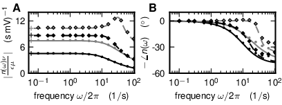

With the general theory developed above we directly obtain an approximation for the colored-noise transfer function , replacing in the white-noise solution (29), denoted by . Here we only consider a modulation of the mean , because it dominates the response properties and briefly discuss a modulation of the variance in the next section. Note that here the modulation enters the equation for . If one is interested in the linear response of the system with respect to a perturbation of the input to , as it appears in the neural context due to synaptic input, one needs to take into account the additional low pass filtering , which is trivial.
A Taylor expansion of the resulting function around the original boundaries reveals the first order correction in
| (30) | ||||
valid for arbitrary noise intensity entering the expression via the boundaries . The first correction term is similar to the -term in (29) indicating that colored noise has a similar effect on the transfer function as a modulation of the variance [48] in the white-noise case. In the high frequency limit this similarity was already found: modulation of the variance leads to finite transmission at infinite frequencies in the white-noise system [48]. The same is true for modulation of the mean in the presence of filtered noise [26]. However, for infinite frequencies our analytical expression behaves differently. The two correction terms in the second line of (30) cancel each other, since and . Thus the transfer function decays to zero as in the white-noise case. This deviation originates from neglecting the time derivative on the left hand side of (10) that is of order , which is true only up to moderate frequencies . The high frequency limit is known explicitly [26], but it was shown that the finite high-frequency transmission is due to the artificial hard threshold in the LIF model [50, 51]. Figure 4 shows a comparison of the analytical prediction (30) to direct simulations for different noise levels and firing rates controlled by the mean . The absolute value of the analytical result is in agreement with simulations for the displayed range of frequencies. Above deviations occur as expected. However, these are less important, since our theory predicts the response properties well in the frequency range where transmission is high. The deviations are more pronounced and already observed at lower frequencies in the phase shift. At high firing rate and low noise, the neuron is mean driven and exhibits a resonance at its firing frequency, again well predicted by the analytical result. The upper row in Figure 5 shows a comparison to the white-noise case. A qualitative change can be observed: synaptic filtering on the one hand increases the dc-susceptibility in contrast to the decreased firing rate (Figure 3A). For this increase is already , implying that this correction is not negligible even for short time constants . On the other hand the cutoff frequency (inset in panel A) is reduced, a behavior which is not expected from the existing knowledge that colored noise enhances the transmission in the high frequency limit. Our theory fully explains these qualitative changes by a shift in the reset and the threshold analogously to the stationary case (Figure 3). This is shown explicitly in panels C and D: for different synaptic time constants the response in the low frequency regime is not altered in comparison to the white-noise case if reset and threshold are adapted according to to compensate for the effect of colored noise.
IV Balanced Random Network
On the network level, the theory of fluctuations (reviewed in [52]) relies on the transfer function as well as the analysis of the stability of networks [53] and of emerging oscillations [34]. With the results from the previous section these collective properties of recurrent networks become analytically accessible for the biologically relevant case of synaptic filtering. We here consider a network consisting of excitatory and inhibitory LIF-model neurons (Section III). The architecture is similar to the one studied in [54] with the extension to synaptic filtering. Each neuron obeys the coupled set of differential equations
| (31) |
corresponding to (18), but with input provided by presynaptic spike trains , where the mark the time points at which neuron emits an action potential, i.e. where exceeds the threshold and denotes the synaptic delay. We use the same neuron parameters as in Figure 5, except a reset of to reduce the impact of an incoming synaptic event, avoiding nonlinear effects. The synaptic weight is for excitatory and for inhibitory synapses. Each excitatory neuron receives excitatory inputs, being the connection probability, and inhibitory inputs drawn randomly and uniformly from the respective populations. Additionally, the neurons receive excitatory and inhibitory external Poisson drive with rates to fix the set point defined by the mean and the standard deviation of the fluctuating input to a cell. Due to homogeneity the excitatory and inhibitory neurons can be summarized into populations with activity , where . In this two-dimensional representation the connectivity can be expressed by the in-degree matrix
A sketch of the network architecture is shown in Figure 6A.
The autospectra and cross-spectra of the population activity can be determined by mapping the system to a linear rate model [52]. The solution is
| (32) |
with the diagonal matrix and the propagator matrix
Here is the weighted transfer function
with given by (25) and identifying , in and given by (29), where we use shifted boundaries (24) to account for the colored noise. Here, we also take into account the contribution to the colored-noise transfer function originating from a modulation of the variance. Its form is again obtained from a shift of the boundaries in the white noise solution , since the general method of reduction (Section II) holds true also for a time-dependent variance as shown in Appendix B.
From (32) we obtain the autospectra of the network activity by a weighted average over the matrix entries
| (33) |
The analytical prediction (33) is in excellent agreement with the spectra obtained in direct simulations of the network (Figure 6). The shape of the power spectra is well captured for different values of and the theory predicts the suppression of fluctuations at frequencies in the low (-) and the high gamma range () caused by synaptic filtering. These frequency bands are related to task dependent activity studied in animals [55] and humans [56]. Although the synaptic time constants are small compared to the membrane time constant (), the influence on the network dynamics is strong. We here present for the first time an analytical argument explaining the effect. The observed deviations at low frequencies are expected: The theory in [52] assumes the autocorrelation of single neurons to be -shaped. This is an approximation likely to be violated, since after reset the membrane potential needs time to recharge, resulting in a dip of the autocorrelation around zero corresponding to a reduction of power at low frequencies. However, the spectrum of the population activity is dominated by cross-correlations resulting in a good overall agreement between theory and simulation. Dummer et al. [57] show that the influence of the cross-correlations on the single neuron’s auto-correlation is negligible and developed an iterative procedure which numerically solves for the self-consistent solution of the auto-correlation. One could incorporate this approach into the theory presented here, replacing the simplified assumption of a -shaped auto-correlation with its self-consistent solution.

V Discussion
In this manuscript we investigate the impact of realistic colored noise on the escape of a Brownian particle from a meta-stable state. Independent of the physical system, specified by the potential, the leading order correction to the escape time solely comes about by the effect of the colored noise in conjunction with the absorbing boundary; there is no correction at the leading order to the Fokker-Planck equation describing the bulk of the density away from the boundary. This is reflected in our generic main result: A time-dependent system driven by colored-noise can to first order be equivalently described by a white-noise system with shifted boundary locations. The modification of the boundary condition can be understood on physical grounds. An absorbing boundary in a white-noise driven system results in a vanishing density at the boundary, because the infinitely fast noise causes any state sufficiently close to the boundary to immediately cross this threshold. The situation is different if the noise has a band-limited spectrum. The diffusive motion induced by the noise is slower, reducing the rate of escape for states close to the boundary. Since the density follows a continuity equation (it obeys conservation of probability), its stationary magnitude results from an equilibrium between inflow and outflow at any instant. A reduced outflow over the threshold is therefore accompanied by elevated density at threshold, which is exactly what is formally achieved by displacing the perfectly absorbing white-noise boundary beyond the point of the physical threshold. This result is in line with the recently observed phenomenon of noise-enhanced stability of a meta-stable state that exhibits a shift of the critical initial position as a function of the color of the noise [58], similar to the shift of the absorbing boundary.
As discussed in Section III.2 the general reduction presented here is valid up to moderate frequencies, while for high frequencies the time derivative on the left hand side of (10) cannot be treated as a second order perturbation in . The presented theory could be extended by absorbing the time derivative into the operator . However, this significantly complicates the form of the outer as well as the boundary-layer solution and the matching between the two. Additionally, the theory could be generalized to multiplicative noise, i.e. an arbitrary factor in front of the noise in (1).
In Section III we apply the central result to the LIF neuron model and obtain an approximation for its transfer function in the presence of colored noise. We show that for biologically relevant parameters the theory presents a viable approximation. In deriving the underlying white-noise transfer function we exploit the analogy between diffusion processes and quantum mechanics by transforming the Fokker-Planck equation of the LIF model to the Hamiltonian of the quantum harmonic oscillator. Besides the technical advantage of using the established operator algebra, this formal analogy exposes that the two components of the transfer function, due to a modulation of the mean input and due to a modulation of the incoming fluctuations, are related to the first and second excited state, respectively, of the quantum harmonic oscillator. These two contributions to the neuronal signal transmission have been studied theoretically [48] and experimentally [59] and the exposed formal analogy casts a new light on this known result. The analytical expression (30) of the transfer function for the colored noise case has immediate applications: The transmission of correlated activity by pairs of neurons exposed to common input [32, 60], can now be studied in a time-resolved manner. Further it enables us to study the effect of synaptic filtering on the oscillatory properties of recurrent networks, as shown in Section IV. More generally, the result allows researchers to map out the phase space (including regions of stability, and the emergence of oscillations) of recurrent neuronal networks, analogous to the white-noise case [54], also in presence of biologically realistic synaptic filtering. This is in particular important as contemporary network models in neuroscience tend to become more and more complex, featuring multiple neuronal populations on the meso- and the macroscopic scale [61, 62]. Having an analytical description at hand allows the identification of sub-circuits critical for the emergence of oscillatory activity and fosters the systematic construction of network models that are in line with experimental observations. In connection with the recently proposed method of linear stability analysis of pulse-coupled oscillators on the basis of perturbations of the inter-event density [63], our modified boundary condition can replace the white noise boundary condition [63, their eq. (9)], to obtain an approximation for the case of colored noise avoiding the need to extend their method to a two-dimensional Fokker-Planck equation.
Excitable systems are ubiquitous in nature and a large body of literature discusses their properties. In particular the escape from a meta-stable state activated by colored noise appears in diverse areas of the natural sciences, including semiconductor physics, physical chemistry, genetics, hydrodynamics and laser physics [16, 17]. The simplicity of the presented method, reducing this general problem to the well understood escape from a potential driven by white-noise, but with displaced boundaries, opens a wide field of applications, where the effect of realistic colored noise can now be accessed in a straight-forward manner.
Acknowledgements.
The authors thank Hannah Bos for substantially contributing to the theory and the simulation code used in Section IV. This work was partially supported by Helmholtz young investigator’s group VH-NG-1028, Helmholtz portfolio theme SMHB, Jülich Aachen Research Alliance (JARA), EU Grant 269921 (BrainScaleS), and EU Grant 604102 (Human Brain Project, HBP). We thank two anonymous referees for their constructive comments which helped us to substantially improve the manuscript. We thank Benjamin Lindner and Nicolas Brunel for helpful comments on an earlier version of the manuscript.References
- [1] H. Kramers, Physica 7, 284 (1940).
- [2] I. Goychuk and P. Hänggi, Proc. Nat. Acad. Sci. USA 99, 3552 (2002), eprint http://www.pnas.org/content/99/6/3552.full.pdf.
- [3] A. Malakhov and A. Pankratov, Physica C: Superconductivity 269, 46 (1996).
- [4] A. L. Pankratov and B. Spagnolo, Phys. Rev. Lett. 93, 177001 (2004).
- [5] R. N. Mantegna and B. Spagnolo, Phys. Rev. Lett. 84, 3025 (2000).
- [6] R. N. Mantegna and B. Spagnolo, Phys. Rev. Lett. 76, 563 (1996).
- [7] J. Hales, A. Zhukov, R. Roy, and M. Dykman, Phys. Rev. Lett. 85, 78 (2000).
- [8] B. Spagnolo, A. Dubkov, A. Pankratov, E. Pankratova, A. Fiasconaro, and A. Ochab-Marcinek, Acta Phys. Pol. B 38, 1925 (2007).
- [9] C. W. Gardiner, Handbook of Stochastic Methods for Physics, Chemistry and the Natural Sciences (Springer-Verlag, Berlin, 1983).
- [10] J. B. Johnson, Phys. Rev. 32, 97 (1928).
- [11] H. Nyquist, Phys. Rev. 32, 110 (1928).
- [12] K. Vogel, T. Leiber, H. Risken, P. Hänggi, and W. Schleich, Phys. Rev. A 35, 4882 (1987).
- [13] U. Frisch and R. Morf, Phys. Rev. A 23, 2673 (1981).
- [14] W. Horsthemke, Noise Induced Transitions, vol. 27 of Springer Series in Synergetics (Springer Berlin Heidelberg, 1984), ISBN 978-3-642-70198-6, URL http://dx.doi.org/10.1007/978-3-642-70196-2_23.
- [15] K. Lindenberg and B. J. West, Physica A 119, 485 (1983).
- [16] F. Moss and P. V. E. McClintock, eds., Noise in Nonlinear Dynamical Systems, vol. 2 (Cambridge University Press, 1989a).
- [17] F. Moss and P. V. E. McClintock, eds., Noise in Nonlinear Dynamical Systems, vol. 3 (Cambridge University Press, 1989b).
- [18] J. M. Sancho, M. SanMiguel, S. L. Katz, and J. D. Gunton, Phys. Rev. A 26, 1589 (1982).
- [19] P. Hanggi, T. J. Mroczkowski, F. Moss, and P. V. E. McClintock, Phys. Rev. A 32, 695 (1985).
- [20] R. F. Fox, Phys. Rev. A 33, 467 (1986).
- [21] P. Grigolini, Phys. Lett. 119, 157 (1986).
- [22] C. R. Doering, P. S. Hagan, and C. D. Levermore, Phys. Rev. Lett. 59, 2129 (1987).
- [23] M. M. Kłosek and P. S. Hagan, J. Math. Phys. 39, 931 (1998).
- [24] L. Lapicque, J. Physiol. Pathol. Gen. 9, 620 (1907).
- [25] R. B. Stein, Biophys. J. 7, 37 (1967).
- [26] N. Brunel, F. S. Chance, N. Fourcaud, and L. F. Abbott, Phys. Rev. Lett. 86, 2186 (2001).
- [27] N. Fourcaud and N. Brunel, Neural Comput. 14, 2057 (2002).
- [28] R. Moreno-Bote and N. Parga, Phys. Rev. Lett. 96, 028101 (2006).
- [29] B. Lindner, Phys. Rev. E 69, 0229011 (2004).
- [30] T. Schwalger, F. Droste, and B. Lindner, Journal of computational neuroscience 39, 29 (2015).
- [31] B. Lindner, B. Doiron, and A. Longtin, Phys. Rev. E 72, 061919 (2005).
- [32] E. Shea-Brown, K. Josic, J. de la Rocha, and B. Doiron, Phys. Rev. Lett. 100, 108102 (2008).
- [33] J. Trousdale, Y. Hu, E. Shea-Brown, and K. Josic, PLOS Computational Biology 8, e1002408 (2012).
- [34] N. Brunel and V. Hakim, Neural Comput. 11, 1621 (1999).
- [35] N. Brunel and X.-J. Wang, J. Neurophysiol. 90, 415 (2003).
- [36] P. Hänggi, P. Talkner, and M. Borkovec, Rev. Mod. Phys. 62, 251 (1990).
- [37] P. Hänggi and P. Jung, Advances in chemical physics 89, 239 (1995).
- [38] P. Hänggi, P. Jung, and P. Talkner, Phys. Rev. Lett. 60, 2804 (1988).
- [39] C. R. Doering, R. J. Bagley, P. S. Hagan, and C. D. Levermore, Phys. Rev. Lett. 60, 2805 (1988).
- [40] H. Risken, The Fokker-Planck Equation (Springer Verlag Berlin Heidelberg, 1996).
- [41] J. Schuecker, M. Diesmann, and M. Helias, arXiv pp. 1410.8799v3 [q–bio.NC] (2014).
- [42] L. Farkas, Z. phys. Chem 125, 236 (1927).
- [43] L. M. Ricciardi, A. Di Crescenzo, V. Giorno, and A. G. Nobile, MathJaponica 50, 247 (1999).
- [44] A. J. Siegert, Phys. Rev. 81, 617 (1951).
- [45] L. M. Ricciardi, Diffusion Processes and Related Topics on Biology (Springer-Verlag, Berlin, 1977).
- [46] http://www.nest simulator.org.
- [47] A. K. Alijani and M. J. E. Richardson, Physical Review E 84, 011919 (2011).
- [48] B. Lindner and L. Schimansky-Geier, Phys. Rev. Lett. 86, 2934 (2001).
- [49] M. Abramowitz and I. A. Stegun, Handbook of Mathematical Functions: with Formulas, Graphs, and Mathematical Tables (Dover Publications, New York, 1974).
- [50] B. Naundorf, T. Geisel, and F. Wolf, arXiv pp. arXiv:physics/0307135 [physics.bio–ph] (2003).
- [51] N. Fourcaud-Trocmé, D. Hansel, C. van Vreeswijk, and N. Brunel, J. Neurosci. 23, 11628 (2003).
- [52] D. Grytskyy, T. Tetzlaff, M. Diesmann, and M. Helias, Front. Comput. Neurosci. 7, 131 (2013).
- [53] L. F. Abbott and C. van Vreeswijk, Phys. Rev. E 48, 1483 (1993).
- [54] N. Brunel, J. Comput. Neurosci. 8, 183 (2000).
- [55] S. Ray, N. E. Crone, E. Niebur, P. J. Franaszczuk, and S. S. Hsiao, J. Neurosci. 28, 11526 (2008), ISSN 1529-2401.
- [56] T. Ball, E. Demandt, I. Mutschler, E. Neitzel, C. Mehring, K. Vogt, A. Aertsen, and A. Schulze-Bonhage, NeuroImage 41, 302 (2008).
- [57] B. Dummer, S. Wieland, and B. Lindner, Front. Comput. Neurosci. 8, 104 (2014).
- [58] A. Fiasconaro and B. Spagnolo, Phys. Rev. E 80, 041110 (2009).
- [59] G. Silberberg, M. Bethge, H. Markram, K. Pawelzik, and M. Tsodyks, J. Neurophysiol. 91, 704 (2004).
- [60] J. De la Rocha, B. Doiron, E. Shea-Brown, J. Kresimir, and A. Reyes, Nature 448, 802 (2007).
- [61] T. C. Potjans and M. Diesmann, Cereb. Cortex 24, 785 (2014), doi: 10.1093/cercor/bhs358.
- [62] M. Schmidt, S. van Albada, R. Bakker, and M. Diesmann, in 2014 Neuroscience Meeting Planner. Washington, DC: Society for Neuroscience. (2014), p. 186.22/TT43.
- [63] F. Farkhooi and C. van Vreeswijk, Phys. Rev. Lett. 115, 038103 (2015).
Appendix A Boundary condition at reset
Certain physical systems, such as biological membranes, exhibit a reset to a smaller value by assigning after has escaped over the threshold. This corresponds to the flux escaping at threshold being re-inserted at reset . The corresponding boundary condition is
With the half-range boundary condition we get
from which we conclude
| (34) |
We now consider the boundary layer at reset described with the rescaled coordinate . We define the boundary layer solution
where we introduced two auxiliary functions and : here is a continuous solution of (3) on the whole domain and, above reset, agrees to the solution that obeys the boundary condition at reset. Correspondingly, the continuous solution agrees to the searched-for solution below reset. With (34) it follows . Thus we have the same boundary condition as in the boundary layer at threshold (11). Therefore the calculations (12)-(15) can be performed analogously, whereby on has to use the continuity of the white-noise solution at reset, i.e. . The result is
a time-dependent boundary condition for the jump of the first-order correction of the outer solution at reset proportional to the probability flux of the white-noise system.
Appendix B Modulation of the noise amplitude
We here show that the reduction from the colored-noise system to the white-noise system presented in Section II can be performed analogously in the case of a temporally modulated noise. To this end we start with the system of equations
where is a time-dependent positive () prefactor modulating the amplitude of the noise. Rescaling both coordinates with the amplitude of the noise and , the temporal derivatives transform to and . After division by and using , we get
where we defined the function appearing in the modified drift term for . The corresponding Fokker-Planck equation (cf. (2) for case with noise of constant amplitude) is
| (35) |
By comparing to (2) we observe that the only formal difference is the additional term . Factoring-off the stationary solution of the fast part with
we obtain (cf. (3))
| (36) | |||||
The additional term affects the perturbation expansion (5) at second order. Since is independent of we have which leads to
Due to , the additional term in the particular solution of the second order is . This term does not contribute to the first order correction of the marginalized probability flux in -direction , because the factor in causes a point-symmetric function in that vanishes after integration over while the factor yields a contribution that is second order in . Therefore the effective flux has the same form as before (8) meaning that the one-dimensional Fokker-Planck equation (9) with replaced with
holds for the case of time-modulated noise. The corresponding SDE is
Transforming back to the original coordinate we get
so that we obtain a SDE with time modulated white noise .
To obtain the boundary condition, we follow the same calculation as in Section II and transform the FPE (36) to the shifted and scaled coordinates , and which yields
| (37) | ||||
with and the operator . Since the additional term is of second order in it only affects the perturbative solution of the second order in (12), so the effective boundary conditions (15) and (16) also hold in the case of time-dependent noise. The reduction of the colored-noise to the corresponding white-noise problem can therefore be performed in the same way as for constant noise.