Nonparametric estimation of extremal dependence

Let $\bm{X}=(X_{1},\ldots,X_{d})$ be a random vector with continuous marginal distribution functions $F_{j}(x_{j})=\mathbb{P}(X_{j}\leq x_{j})$ and joint distribution function $F(\bm{x})=\mathbb{P}(X_{1}\leq x_{1},\ldots,X_{d}\leq x_{d})$. To study tail dependence, we zoom in on the joint distribution of $(F_{1}(X_{1}),\ldots,F_{d}(X_{d}))$ in the neighbourhood of its upper endpoint $(1,\ldots,1)$. That is, we look at

where $t>0$ is small and where the numbers $x_{1},\ldots,x_{d}\in[0,\infty)$ parametrize the relative distances to the upper endpoints of the $d$ variables. The above probability converges to zero as $t\to 0$ and is in fact proportional to $t$:

The stable tail dependence function, $\ell:[0,\infty)^{d}\rightarrow[0,\infty)$, is then defined by

for $\bm{x}\in[0,\infty)^{d}$ (Huang, 1992; Drees and Huang, 1998). The existence of the limit in (4) is an assumption that can be tested (Einmahl et al., 2006).

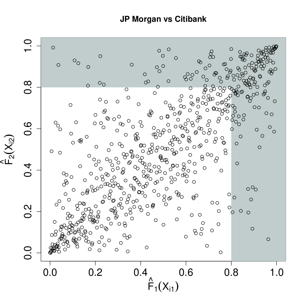
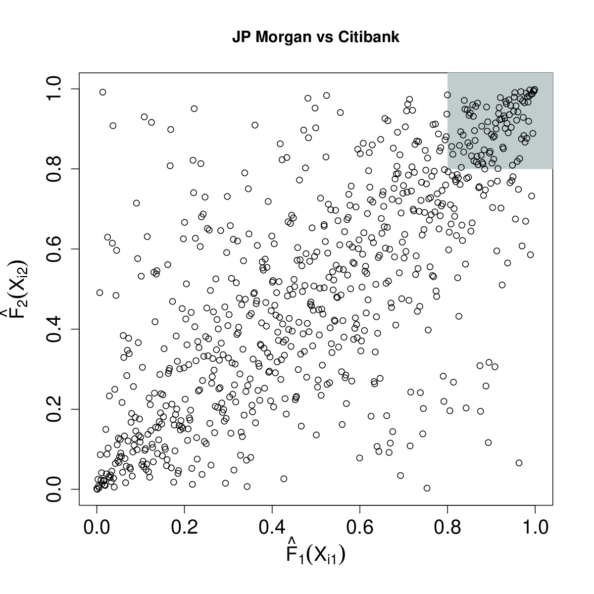
The probability in (3) represents the situation where at least one of the variables is large: for instance, the sea level exceeds a critical height at one or more locations. Alternatively, we might be interested in the situation where all variables are large simultaneously. Think of the prices of all stocks in a financial portfolio going down together. The tail copula, $R:[0,\infty)^{d}\to[0,\infty)$, is defined by

for $\bm{x}\in[0,\infty]^{d}\setminus\{(\infty,\ldots,\infty)\}$. Again, existence of the limit is an assumption. In the bivariate case ($d=2$), the functions $\ell$ and $R$ are directly related by $R(x,y)=x+y-\ell(x,y)$. The difference between $\ell$ and $R$ is visualized in Figure 2 for the log-returns of the stock prices of JP Morgan versus Citibank. From now on, we will focus on the function $\ell$ because of its direct link to the joint distribution function; see (6).

It is convenient to transform the random variables $X_{1},\ldots,X_{j}$ to have the unit-Pareto distribution via the transformations $X_{j}^{*}=1/\{1-F_{j}(X_{j})\}$ for $j=1,\ldots,d$. The existence of $\ell$ in (4) is equivalent to the statement that the joint distribution function, $H_{0}$, of the random vector $\bm{X}^{*}=(X_{1}^{*},\ldots,X_{d}^{*})$ is in the max-domain of attraction of a $d$-variate extreme-value distribution, say $G_{0}$, with unit-Fréchet margins, i.e., $G_{0j}(z_{j})=\exp(-1/z_{j})$ for $z_{j}>0$. The link between $\ell$ and $G_{0}$ is given by

so that $G_{0}(\bm{z})=\exp{\{-\ell(1/z_{1},\ldots,1/z_{d})\}}$. Since, for “large” $z_{1},\ldots,z_{d}$ we have

we see that estimating the stable tail dependence function $\ell$ is key to estimation of the tail of $H_{0}$, and thus, after marginal transformation, of $F$. If, in addition, the marginal distributions $F_{1},\ldots,F_{d}$ are in the max-domains of attraction of the univariate extreme-value distributions $G_{1},\ldots,G_{d}$, then $F$ is in the max-domain of attraction of the $d$-variate extreme-value distribution $G(\bm{x})=\exp\{-\ell(-\log G_{1}(x_{1}),\ldots,-\log G_{d}(x_{d}))\}$.

Every stable tail dependence function $\ell$ has the following properties:

1. 1.

   $\max{(x_{1},\ldots,x_{d})}\leq\ell(\bm{x})\leq x_{1}+\cdots+x_{d}$, and in particular $\ell(0,\ldots,0,x_{j},0,\ldots,0)=x_{j}$ for $j=1,\ldots,d$;

2. 2.

   convexity, that is, $\ell\bigl(t\bm{x}+(1-t)\bm{y}\bigr)\leq t\,\ell(\bm{x})+(1-t)\,\ell(\bm{y})$, for $t\in[0,1]$;

3. 3.

   order-one homogeneity: $\ell(ax_{1},\ldots,ax_{d})=a\,\ell(x_{1},\ldots,x_{d})$, for $a>0$;

(Beirlant et al., 2004, page 257). When $d=2$, these three properties characterize the class of stable tail dependence functions. When $d\geq 3$, a function satisfying these properties is not necessarily a stable tail dependence function.

The two boundary cases are complete dependence, $\ell(\bm{x})=\max(x_{1},\ldots,x_{d})$, and independence, $\ell(\bm{x})=x_{1}+\cdots+x_{d}$. Another example is the logistic model,

As $\theta\rightarrow 1$, extremes become independent and as $\theta\rightarrow\infty$, extremes become completely dependent. The copula of the extreme-value distribution $G_{0}$ with this stable tail dependence function is the Gumbel–Hougaard copula.

The stable tail dependence function is related to two other functions:

• •

  The exponent measure function $V(\bm{z})\coloneqq-\log G_{0}(\bm{z})=\ell(1/z_{1},\ldots,1/z_{d})$, for $\bm{z}\in(0,\infty]^{d}$ (Coles and Tawn, 1991).

• •

  The Pickands dependence function $A$, which is just the restriction of $\ell$ to the unit simplex $\{\bm{x}\in[0,\infty)^{d}:x_{1}+\cdots+x_{d}=1\}$ (Pickands, 1981). In dimension $d=2$, it is common to set $A(t)=\ell(1-t,t)$ for $t\in[0,1]$.

Another insightful approach for modelling extremal dependence of a $d$-dimensional random vector is to look at the contribution of each of the $d$ components to their sum conditionally on the sum being large.

Consider first the bivariate case. In Figure 3 we show pseudo-random samples from the Gumbel copula, which is related to the logistic model (7), at two different values of the dependence parameter $\theta$: strong dependence ($\theta=2.5$) at the top and weak dependence ($\theta=1.25$) at the bottom. For convenience, the axes in the scatter plots on the left are on the logarithmic scale. The points for which the sum of the coordinates belong to the top-10% are shown in black. In the middle panels we plot the ratio of the first component to the sum (horizontal axis) against the sum itself (vertical axis). On the right, finally, histograms are given of these ratios for those points for which the sum exceeded the threshold in the plots on the left and in the middle. Strong extremal dependence leads to the ratios being close to $0.5$ (top), whereas low extremal dependence leads to the ratios being close to either $0$ or $1$ (bottom).

We learn that the distribution of the ratios of the components to their sum, given that the sum is large, carries information about dependence between large values. This distribution is called the angular or spectral measure (de Haan and Resnick, 1977) and is denoted here by $H$. The reference lines in Figure 3 represent the spectral density associated with the Gumbel copula with parameter $\theta>1$, that is,

In Figure 4 we show the same plots as in Figure 3 but now for the pairs of negative log-returns of the stock prices of JP Morgan versus Citibank (top) and JP Morgan versus IBM (bottom). For each of the two pairs we do the following. Let $(X_{i},Y_{i})$, $i=1,\ldots,n$, denote a bivariate sample. First, we transform the data to the unit-Pareto scale using and (1) and (2), i.e.,

Here $R_{i,X}$ is the rank of $X_{i}$ among $X_{1},\ldots,X_{n}$ and $R_{i,Y}$ is the rank of $Y_{i}$ among $Y_{1},\ldots,Y_{n}$. Next, we construct an approximate sample from the spectral measure $H$ by setting

The data in the pseudo-polar representation (9) are shown in the middle plots. The histograms of the ratios $\widehat{W}_{i}$ for those points for which the sum $\widehat{S}_{i}$ is above the $95\%$ sample quantile are displayed on the right-hand side. The solid black lines show the smoothed spectral density estimator in (21) below.

For JP Morgan versus Citibank, the ratios are spread equally across the unit interval, suggesting extremal dependence. In contrast, for JP Morgan versus IBM, the spectral density has peaks at the boundaries $0$ and $1$, suggesting weak extremal dependence.

In the general, $d$-dimensional setting we transform the random vector $\bm{X}^{*}=(X_{1}^{*},\ldots,X_{d}^{*})=(1/\{1-F_{j}(X_{j})\}:j=1,\ldots,d)$ as follows:

The spectral measure is defined as the asymptotic distribution of the vector of ratios $\bm{W}$ given that the sum $S$ is large:

The support of $H$ is included in the unit simplex $\Delta_{d-1}=\{\bm{w}\in[0,\infty)^{d}:w_{1}+\cdots+w_{d}=1\}$. In case of asymptotic independence, the spectral measure is concentrated on the $d$ vertices of $\Delta_{d-1}$, whereas in case of complete asymptotic dependence it reduces to a unit point mass at the center of $\Delta_{d-1}$.

The spectral measure is related to the stable tail dependence function via

The property that $\ell(0,\ldots,0,1,0,\ldots,0)=1$ implies the moment constraints

Taking these constraints into account helps to improve the efficiency of nonparametric estimators of $H$ (Section 3.1).

Any probability measure on the unit simplex satisfying (13) can be shown to be a valid spectral measure. The family of stable tail dependence functions is then characterized by (12) via a certain integral transform of such measures.

Let $(X_{i},Y_{i})$, $i=1,\ldots,n$, be independent copies of a random vector $(X,Y)$ with distribution function $F$ and continuous marginal distribution functions $F_{X}$ and $F_{Y}$. Assume that $F$ has a stable tail dependence function $\ell$ as in (24). The function $\ell$ can be represented by the spectral measure $H$ via (12), which in the bivariate case specializes to

the unit simplex in $\mathbb{R}^{2}$ being identified with the unit interval, $[0,1]$. The moment constraints in (13) simplify to

The aim here is to estimate the spectral measure $H$. The starting point is the limit relation (11). Standardize the margins to the unit-Pareto distribution via $X^{*}=1/\{1-F_{X}(X)\}$ and $Y^{*}=1/\{1-F_{Y}(Y)\}$ and write

Equation (11) then becomes

The spectral measure $H$ can be interpreted as the limit distribution of the angular component, $W$, given that the radial component, $S$, is large.

Mimicking the transformation from $(X,Y)$ via $(X^{*},Y^{*})$ to $(S,W)$ in a given data-set, it is convenient to standardize the data to the unit-Pareto distribution via (8) and then switch to pseudo-polar coordinates using (9). Different choices for the angular components are possible; for example, Einmahl and Segers (2009) use $\arctan(X^{*}/Y^{*})$. For the radial component one can take in general the $L_{p}$ norm, $p\in[1,+\infty]$; Einmahl et al. (2001) take the $L_{\infty}$ norm and de Carvalho et al. (2013) take the $L_{1}$ norm. Note however that different normalizations lead to different spectral measures.

For estimation purposes, transform pairs $(X_{i},Y_{i})$ into $(\widehat{S}_{i},\widehat{W}_{i})$ as in (8) and (9). Set the threshold $u$ in (16) to $n/k$, where $k=k_{n}\in(0,n]$ is an intermediate sequence such that $k\to\infty$ and $k/n\to 0$ as $n\to\infty$. Let $I_{n}=\{i=1,\ldots,n:\;\widehat{S}_{i}\geq n/k\}$ denote the set of indices that correspond to the observations with pseudo-radial component $\widehat{S}_{i}$ above a high threshold, and let $N_{n}=\left\lvert{I_{n}}\right\rvert$ denote its cardinality. Here we specify $u$ as the $95\%$ quantile of $\widehat{S}_{i}$.

In the literature, three nonparametric estimators of the spectral measure have been proposed. All three are of the form

The estimators distinguish themselves in the way the weights $\widehat{p}_{l,i}$ are defined.

For the empirical spectral measure (Einmahl et al., 2001), the weights are set to be constant, i.e., $\widehat{p}_{1,i}=1/N_{n}$. The estimator $\widehat{H}_{1}$ (17) becomes an empirical version of (16). However, this estimator does not necessarily satisfy the moment constraints in (15). This is a motivation for the two other estimators where the moment constraint is enforced by requiring that $\sum_{i\in I_{n}}\widehat{W}_{i}\widehat{p}_{l,i}=1/2$.

The maximum empirical likelihood estimator (Einmahl and Segers, 2009), $\widehat{H}_{2}\left(x\right)$, has probability masses $\widehat{p}_{2,i}$ solving the optimization problem

By construction, the weights $\widehat{p}_{2,i}$ satisfy the moment constraints. The optimization problem in (18) can be solved by the method of Lagrange multipliers. In the nontrivial case where $1/2$ is in the convex hull of $\{W_{i}:i\in I_{n}\}$, the solution is given by

where $\lambda\in\mathbb{R}$ is the Lagrange multiplier associated to the second equality constraint in (18), defined implicitly as the solution to the equation

Note that in (18), it is implicitly assumed that $\widehat{p}_{2,i}>0$.

Another estimator that satisfies the moment constraints is the maximum Euclidean likelihood estimator (de Carvalho et al., 2013). The probability masses $\widehat{p}_{3,i}$ solve the following optimization problem:

This quadratic optimization problem with linear constraints can be solved explicitly with the method of Lagrange multipliers, yielding

where $\overline{W}$ and $S_{W}^{2}$ denote the sample mean and sample variance of $\widehat{W}_{i}$, $i\in I_{n}$, respectively, that is,

The weights $\widehat{p}_{3,i}$ could be negative, but this does usually not occur as the weights are all nonnegative with probability tending to one.

It is shown in Einmahl and Segers (2009) and de Carvalho et al. (2013) that $\widehat{H}_{2}\left(x\right)$ and $\widehat{H}_{3}\left(x\right)$ are more efficient than $\widehat{H}_{1}\left(x\right)$. Moreover, asymptotically there is no difference between the maximum empirical likelihood or maximum Euclidean likelihood estimators. The maximum Euclidean likelihood estimator is especially convenient as the weights $\widehat{p}_{3,i}$ are given explicitly.

For the stock market data from JP Morgan, Citibank and IBM, Figure 5 shows the empirical spectral measure $\widehat{H}_{1}\left(x\right)$ and the maximum Euclidean estimator $\widehat{H}_{3}\left(x\right)$ for the two pairs involving JP Morgan. In each case, the threshold $u$ is set to be the $95\%$ quantile of the sample of radii $\widehat{S}_{i}$. Enforcing the moment constraints makes a small but noticeable difference. Tail dependence is strongest for the pair JP Morgan versus Citibank, with spectral mass distributed approximately uniformly over $[0,1]$. For the pair JP Morgan versus IBM, tail dependence is weaker, the spectral measure being concentrated mainly near the two endpoints, $0$ and $1$.

The nonparametric estimators of the spectral probability measure can be smoothed in such a way that the smoothed versions still obey the moment constraints. This can be done using kernel smoothing techniques, although some care is needed since the spectral measure is defined on a compact interval. In de Carvalho et al. (2013) the estimator is constructed by combining Beta distributions with the weights, $\widehat{p}_{3,i}$, of the maximum Euclidean likelihood estimate. To ensure that the estimated measure obeys the marginal moment constraints, it is imposed that the mean of each smoother equals the observed pseudo-angle. The Euclidean spectral density estimator is defined as

where $\nu>0$ is the smoothing parameter, to be chosen via cross-validation, and

is the Beta density with parameters $p,q>0$.

For the financial data, the realized spectral density estimator $\widetilde{h}_{3}(x)$ is plotted on the right-hand panel of Figure 4. The picture is in agreement with the one in Figure 5. The distribution of the spectral mass points to asymptotic dependence for JP Morgan versus Citibank and to weaker asymptotic dependence for JP Morgan versus IBM.

Integrating out the estimated spectral density yields a smoothed version of the empirical spectral measure or its variants: for the maximum Euclidean likelihood estimator, we get

with $\mathcal{B}(x;p,q)=\int_{0}^{x}\beta(y;p,q)\,\mathrm{d}y$ the regularized incomplete beta function. As

the moment constraint (15) is satisfied.

Consider again the general, multivariate case. Given a random sample $\bm{X}_{i}=(X_{i1},\ldots,X_{id})$, $i=1,\ldots,n$, the aim is to estimate the stable tail dependence function $\ell$ in (4) of the common distribution $F$ with continuous margins $F_{1},\ldots,F_{d}$. A straightforward nonparametric estimator can be defined as follows. Let $k=k_{n}\in\{1,\ldots,n\}$ be such that $k\to\infty$ and $k/n\to 0$ as $n\to\infty$. By replacing $\mathbb{P}$ by the empirical distribution function, $t$ by $k/n$, and $F_{1},\ldots,F_{d}$ by $\widehat{F}_{1},\ldots,\widehat{F}_{d}$ as defined in (2), we obtain the empirical tail dependence function (Huang, 1992; Drees and Huang, 1998)

Under minimal assumptions, the estimator is consistent and asymptotically normal with a convergence rate of $\sqrt{k}$ (Einmahl et al., 2012; Bücher et al., 2014). Alternatively, the marginal distributions might be estimated by $\widehat{F}_{j,2}(X_{ij})=R_{ij,n}/n$ or $\widehat{F}_{j,3}(X_{ij})=(R_{ij,n}-1/2)/n$, resulting in estimators that are asymptotically equivalent to $\widehat{\ell}$.

Another estimator of $\ell$ can be defined by estimating the spectral measure, $H$, and applying the transformation in (12), an idea going back to Capéraà and Fougères (2000). In the bivariate case, we can replace $H$ in (14) by one of the three nonparametric estimators $\widehat{H}_{l}$ studied in Section 3.1. Recall the notations in (8) and (9). If we modify the definition of the index set $I_{n}$ to $I_{n}=\{i=1,\ldots,n:\widehat{S}_{i}>\widehat{S}_{(k+1)}\}$, where $\widehat{S}_{(k+1)}$ denotes the $(k+1)$-th largest observation of the $\widehat{S}_{i}$’s, then there are exactly $k$ elements in the set $I_{n}$. Starting from the empirical spectral measure $\widehat{H}_{1}$, we obtain the estimator

For the maximum empirical or Euclidean likelihood estimators $\widehat{H}_{2}$ and $\widehat{H}_{3}$, one needs to replace the factor $1/k$ by the weights $\widehat{p}_{2,i}$ and $\widehat{p}_{3,i}$, respectively.

A way to visualize the function $\ell$ or an estimator thereof is via the level sets $\mathcal{D}_{c}\coloneqq\{(x,y):\ell(x,y)=c\}$ for a range of value of $c>0$. Note that the level sets are equal to the lines $x+y=c$ in case of asymptotic independence and to the elbow curves $\max(x,y)=c$ in case of complete asymptotic dependence. Likewise, a plot of the level sets of an estimator of $\ell$ can be used as a graphical diagnostic of asymptotic (in)dependence; see de Haan and de Ronde (1998) or de Haan and Ferreira (2006, Section 7.2).

We plot the lines $\mathcal{D}_{c}$ for $c\in\{0.2,0.4,0.6,0.8,1\}$ and $k=50$ of $\widehat{\ell}$ and $\widehat{\ell}_{CF}$ for the weekly log-returns of JP Morgan versus Citibank and JP Morgan versus IBM in Figure 6. The level sets for JP Morgan versus IBM resemble the straight lines $x+y=c$ much more closely than the level sets for JP Morgan versus Citibank do. The estimator based on the spectral measure, $\widehat{\ell}_{CF}$, acts as a smooth version of the empirical tail dependence function $\widehat{\ell}$.

Nonparametric estimators for $\ell$ can also serve as stepping stone for semiparametric inference. Assume that $\ell=\ell_{\theta_{0}}\in\{\ell_{\theta}:\theta\in\Theta\}$, a finite-dimensional parametric family. Then one could estimate $\theta_{0}$ by minimizing a distance or discrepancy measure between $\hat{\ell}$ and members of the parametric family (Einmahl et al., 2012; Einmahl et al., 2014).

A first measure for the strength of asymptotic dependence is the tail dependence coefficient

(Coles et al., 1999). By the properties of $\ell$ (Section 2.1), we have $\ell(x,y)=x+y$ for all $(x,y)$ if and only if $\ell(1,1)=2$. That is, asymptotic independence is equivalent to $\chi=0$, whereas asymptotic dependence is equivalent to $\chi\in(0,1]$.

To estimate $\chi$, we will first write it as the limit of a function $\chi(u)$, so that $\lim_{u\uparrow 1}\chi(u)=\chi$; the function $\chi(u)$ is defined as

To estimate $\chi(u)$ from a sample $(X_{1},Y_{1}),\ldots,(X_{n},Y_{n})$, simply replace $F_{X}$ and $F_{Y}$ by their empirical counterparts in (2):

For the stock price log-returns of JP Morgan, Citibank, and IBM, the estimated tail dependence coefficients $\widehat{\chi}(u)$ of the three possible pairs are shown in Figure 7 as a function of $u\geq 0.8$. The plot confirms the earlier finding that tail dependence is stronger between the two banking stocks, JP Morgan and Citibank, than between either of the two banks and IBM.

If the variables are asymptotically independent, $\chi=0$, we need a second measure quantifying the extremal dependence. The coefficient of tail dependence, $\eta$, can be motivated as follows (Ledford and Tawn, 1996). Since $\mathbb{P}[1/\{1-F_{X}(X)\}>t]=1/t$ for $t\geq 1$, we have

A model that links these two situations is given by the assumption that the joint survival function above is regularly varying at $\infty$ with index $-1/\eta$, i.e.,

where $\mathcal{L}$ is a slowly varying function, that is, $\mathcal{L}(tr)/\mathcal{L}(t)\to 1$ as $t\to\infty$ for fixed $r>0$; see for example Resnick (1987).

For large $t$, if we treat $\mathcal{L}$ as constant, there are three cases of non-negative extremal association to distinguish:

1. 1.

   $\eta=1$ and $\mathcal{L}(t)\to c>0$: asymptotic dependence;

2. 2.

   $1/2<\eta<1$: positive association within asymptotic independence;

3. 3.

   $\eta=1/2$: (near) perfect independence.

Values of $\eta<1/2$ occur when there is negative association between the two random variables at extreme levels.

In order to estimate $\eta$, we first define the structure variable

For a high threshold $u$ and for $t\geq 0$, we have, by slow variation of $\mathcal{L}$,

On the right-hand side we recognize a generalized Pareto distribution with shape parameter $\eta$. Given the sample $(X_{1},Y_{1}),\ldots,(X_{n},Y_{n})$, we can estimate $\eta$ with techniques from univariate extreme value theory applied to the variables

One possibility consists of fitting the generalized Pareto distribution to the sample of excesses $\widehat{T}_{i}-u$ for those $i$ for which $\widehat{T}_{i}>u$ (Ledford and Tawn, 1996, page 180). Alternatively, one can use the Hill estimator (Hill, 1975)

where $\widehat{T}_{(1)}\geq\cdots\geq\widehat{T}_{(n)}$ denote the order statistics of $\widehat{T}_{1},\ldots,\widehat{T}_{n}$. Figure 7 shows the estimators $\widehat{\eta}_{H}$ of the coefficient of tail dependence between JP Morgan and Citibank, JP Morgan and IBM, and Citibank and IBM for a decreasing number of order statistics. The estimators suggest asymptotic dependence for the log-returns of JP Morgan versus Citibank.

Another frequently used measure in case of asymptotic independence can be obtained from (26). Taking logarithms on both sides and using slow variation of $\mathcal{L}$, we obtain

Coles et al. (1999) proposed the coefficient

As $0<\eta\leq 1$, we have $-1<\overline{\chi}\leq 1$. For a bivariate normal dependence structure, $\overline{\chi}$ is equal to the correlation coefficient $\rho$. Together, the two coefficients $\chi$ and $\overline{\chi}$ contain complementary information on the amount of tail dependence:

REFERENCES

- Bacro and Toulemonde (2013) Bacro, J.-N. and G. Toulemonde (2013). Measuring and modelling multivariate and spatial dependence of extremes. Journal de la Société Française de Statistique 154(2), 139–155.
- Beirlant et al. (2004) Beirlant, J., Y. Goegebeur, J. Segers, and J. Teugels (2004). Statistics of Extremes: Theory and Applications. Wiley.
- Bücher et al. (2014) Bücher, A., J. Segers, and S. Volgushev (2014). When uniform weak convergence fails: empirical processes for dependence functions and residuals using epi- and hypographs. The Annals of Statistics (to appear), http://arxiv.org/abs/1305.6408.
- Capéraà and Fougères (2000) Capéraà, P. and A.-L. Fougères (2000). Estimation of a bivariate extreme value distribution. Extremes 3(4), 311–329.
- Coles et al. (1999) Coles, S., J. Heffernan, and J. Tawn (1999). Dependence measures for extreme value analyses. Extremes 2(4), 339–365.
- Coles and Tawn (1991) Coles, S. and J. Tawn (1991). Modelling extreme multivariate events. Journal of the Royal Statistical Society: Series B (Statistical Methodology) 53, 377–392.
- de Carvalho et al. (2013) de Carvalho, M., B. Oumow, J. Segers, and M. Warchoł (2013). A euclidean likelihood estimator for bivariate tail dependence. Communications in Statistics - Theory and Methods 42(7), 1176–1192.
- de Carvalho and Ramos (2012) de Carvalho, M. and A. Ramos (2012). Bivariate extreme statistics, ii. REVSTAT - Statistical Journal 11(1), 83–107.
- de Haan and de Ronde (1998) de Haan, L. and J. de Ronde (1998). Sea and wind: Multivariate extremes at work. Extremes 1, 7–45.
- de Haan and Ferreira (2006) de Haan, L. and A. Ferreira (2006). Extreme Value Theory: an Introduction. Springer-Verlag Inc.
- de Haan and Resnick (1977) de Haan, L. and S. I. Resnick (1977). Limit theory for multivariate sample extremes. Z. Wahrscheinlichkeitstheorie und Verw. Gebiete 40(4), 317–337.
- Draisma et al. (2004) Draisma, G., H. Drees, A. Ferreira, and L. De Haan (2004). Bivariate tail estimation: dependence in asymptotic independence. Bernoulli 10(2), 251–280.
- Drees and Huang (1998) Drees, H. and X. Huang (1998). Best attainable rates of convergence for estimators of the stable tail dependence function. Journal of Multivariate Analysis 64(1), 25–47.
- Einmahl et al. (2006) Einmahl, J., L. de Haan, and D. Li (2006). Weighted approximations of tail copula processes with application to testing the bivariate extreme value condition. The Annals of Statistics 34, 1987–2014.
- Einmahl et al. (2014) Einmahl, J., A. Kiriliouk, A. Krajina, and J. Segers (2014). An M-estimator of spatial tail dependence. Available on http://arxiv.org/abs/1403.1975.
- Einmahl et al. (2012) Einmahl, J., A. Krajina, and J. Segers (2012). An M-estimator for tail dependence in arbitrary dimensions. The Annals of Statistics 40, 1764–1793.
- Einmahl et al. (2001) Einmahl, J. H., L. de Haan, and V. I. Piterbarg (2001). Nonparametric estimation of the spectral measure of an extreme value distribution. The Annals of Statistics 29(5), 1401–1423.
- Einmahl and Segers (2009) Einmahl, J. H. J. and J. Segers (2009). Maximum empirical likelihood estimation of the spectral measure of an extreme-value distribution. The Annals of Statistics 37(5B), 2953–2989.
- Falk et al. (2011) Falk, M., J. Hüsler, and R.-D. Reiss (2011). Laws of small numbers: extremes and rare events (extended ed.). Birkhäuser/Springer Basel AG, Basel.
- Fisher and Tippett (1928) Fisher, R. A. and L. H. C. Tippett (1928). Limiting forms of the frequency distribution of the largest or smallest member of a sample. In Mathematical Proceedings of the Cambridge Philosophical Society, Volume 24, pp. 180–190. Cambridge Univ Press.
- Gnedenko (1943) Gnedenko, B. (1943). Sur la distribution limite du terme maximum d’une serie aleatoire. Annals of mathematics, 423–453.
- Heffernan and Stephenson (2012) Heffernan, J. E. and A. G. Stephenson (2012). ismev: An Introduction to Statistical Modeling of Extreme Values. R package version 1.38.
- Hill (1975) Hill, B. M. (1975). A simple general approach to inference about the tail of a distribution. The Annals of Statistics 3, 1163–1174.
- Huang (1992) Huang, X. (1992). Statistics of bivariate extreme values. Ph. D. thesis, Tinbergen Institute Research Series.
- Hüsler and Li (2009) Hüsler, J. and D. Li (2009). Testing asymptotic independence in bivariate extremes. Journal of Statistical Planning and Inference 139, 990–998.
- Ledford and Tawn (1996) Ledford, A. W. and J. A. Tawn (1996). Statistics for near independence in multivariate extreme values. Biometrika 83, 169–187.
- Pickands (1981) Pickands, J. (1981). Multivariate extreme value distributions. In Bulletin of the International Statistical Institute, pp. 859–878.
- Resnick (1987) Resnick, S. I. (1987). Extreme Values, Regular Variation, and Point Processes. Springer, New York.
- Segers (2012) Segers, J. (2012). Max-stable models for multivariate extremes. REVSTAT Statistical Journal 10, 61–82.
- Sibuya (1960) Sibuya, M. (1960). Bivariate extreme statistics, I. Annals of the Institute of Statistical Mathematics 11(2), 195–210.