Are the small neutrino oscillation parameters all related?

Information on neutrino mass and mixing have been steadily emerging from oscillation experiments. Among them the angle¹¹ 1 For the lepton mixing matrix the standard PMNS form is used. $\theta_{13}$ is small ($\sin\theta_{13}\sim 0.1$) [1] while global fits to the solar, atmospheric, accelerator, and reactor neutrino oscillation data indicate that $\theta_{23}$ is near maximal ($\sim\pi/4$) [2, 3]. On the other hand, the solar mass square difference is two orders smaller than the atmospheric one. These mixing parameters and the mass ordering are essential inputs for identifying viable models for neutrino masses.

A natural choice could be to take the mixing angles to be initially either $\pi/4$ ($\theta_{23}$) or zero ($\theta_{13}$, $\theta_{12}$) and the solar splitting absent. In this spirit, here a proposal is put forward under which the atmospheric mass splitting and maximal mixing in this sector arise from a zero-order mass matrix while the smaller solar mass splitting and realistic $\theta_{13}$ and $\theta_{23}$ are generated by a Type-I see-saw [4] which acts as a perturbation. $\theta_{12}$ also arises out of the same perturbation and as a consequence of degeneracy is not constrained to be small. Attempts to generate some of the neutrino parameters by perturbation theory are not new [5, 6], but to our knowledge there is no work in the literature that indicates that all the small parameters could have the same perturbative origin and agree with the current data.

The unperturbed neutrino mass matrix in the mass basis is $M^{0}={\rm diag}\{m^{(0)}_{1},m^{(0)}_{1},m^{(0)}_{3}\}$ with the mixing matrix of the form

Here $\Delta m^{2}_{atm}=(m^{(0)}_{3})^{2}-(m^{(0)}_{1})^{2}$. By suitably choosing the Majorana phases the masses $m^{(0)}_{1},m^{(0)}_{3}$ are taken to be real and positive. The columns of $U^{0}$ are the unperturbed flavour eigenstates²² 2 In the flavour basis the charged lepton mass matrix is diagonal.. As stated, $\Delta m^{2}_{solar}=0$ and $\theta_{13}=0$. Since the first two states are degenerate in mass, one can also take $\theta_{12}=0$. It is possible to generate this mass matrix from a Type-II see-saw.

In the flavour basis the mass matrix is $(M^{0})^{flavour}=U^{0}M^{0}U^{0T}$ which in terms of $m^{\pm}=m_{3}^{(0)}\pm m_{1}^{(0)}$ is

The perturbation is obtained by a Type-I see-saw. To reduce the number of independent parameters, in the flavour basis the Dirac mass term is taken to be proportional to the identity, i.e.,

In this basis, in the interest of minimality the right-handed neutrino Majorana mass matrix is taken with only two non-zero complex entries.

where $x,y$ are dimensionless constants of ${\cal O}(1)$. No generality is lost by keeping the Dirac mass real.

As a warm-up consider first the real case, i.e., $\phi_{1}=0~{\rm or}~\pi,\phi_{2}=0~{\rm or}~\pi$. For notational convenience in the following the phase factors are not displayed; instead $x$ ($y$) is taken as positive or negative depending on whether $\phi_{1}$ ($\phi_{2}$) is 0 or $\pi$. Negative $x$ and $y$ offer interesting variants which are stressed at the appropriate points.

The Type-I see-saw contribution in the mass basis is:

The effect on the solar sector is governed by the submatrix of $M^{\prime mass}$ in the subspace of the two degenerate states,

To first order in the perturbation:

For $y/x=1$ one obtains the tribimaximal mixing value of $\theta_{12}$ which, though allowed by the data³³ 3 We use the 3$\sigma$ ranges $7.03\leq\Delta m_{21}^{2}/10^{-5}\,{\rm eV}^{2}\leq 8.03\;\;{\rm and}\;\;31.30^{\circ}\leq\theta_{12}\leq 35.90^{\circ}$ [2]. at 3$\sigma$, is beyond the $1\sigma$ region. Since for the entire range of $\theta_{12}$ one has $\tan 2\theta_{12}>0$, $x$ and $y$ must be chosen of the same sign. Therefore, either $\phi_{1}=0=\phi_{2}$ or $\phi_{1}=\pi=\phi_{2}$. From the global fits to the experimental results one finds:

Further, from eq. (6),

To first order in the perturbation the corrected wave function $|\psi_{3}\rangle$ is:

where

For positive $x$ the sign of $\kappa$ is fixed by that of $m^{-}$. Since by convention all the mixing angles $\theta_{ij}$ are in the first quadrant, from eq. (10) one must identify:

where for $x>0$ the PMNS phase $\delta=0$ for normal mass ordering (NO) and $\delta=\pi$ for inverted mass ordering (IO). Needless to say, both these cases are CP conserving. If $x$ is negative then NO (IO) would correspond to $\delta=\pi~(0)$.

An immediate consequence of eqs. (12), (7), and (9) is

which exhibits how the solar sector and $\theta_{13}$ are intertwined. The positive sign of $\Delta m^{2}_{solar}$, preferred by the data, is trivially verified since ${\rm sgn}(x)~m^{-}\sin\theta_{13}\cos\delta>0$ from eq. (12). However, eq. (13) excludes inverted ordering. Once the neutrino mass square splittings, $\theta_{12}$, and $\theta_{13}$ are chosen, eq. (13) determines the lightest neutrino mass, $m_{0}$. Defining $z=m^{-}m^{(0)}_{1}/\Delta m^{2}_{atm}$ and $m_{0}/\sqrt{|\Delta m^{2}_{atm}|}=\tan\xi$, one has

It is seen that $0\leq z\leq 1/2$ for NO and $1/2\leq z\leq 1$ for IO, with $z\rightarrow 1/2$ corresponding to quasidegeneracy, i.e., $m_{0}\rightarrow$ large, in both cases. From eq. (13)

with $|\cos\delta|=1$ for real $M_{R}$. As shown below, the allowed ranges of the oscillation parameters imply $z\sim 10^{-2}$ and so inverted mass ordering is disallowed.

From eq. (10) one further finds:

where, using eqs. (7) and (12),

$\theta_{23}$ will be in the first (second) octant, i.e., the sign of $\omega$ will be positive (negative) if $\delta=0~(\pi)$. Recall, this corresponds to $x>0$ ($x<0$).

In Fig. 1 the global-fit 3$\sigma$ range of $\sin\theta_{13}$ and $\tan 2\theta_{12}$ is shown as the blue dot-dashed box with the best-fit value indicated by a black dot. Once the atmospheric and solar mass splittings are fixed, for any point within this region eq. (15) determines a $z$, or equivalently an $m_{0}$, which leads to the correct solar splitting.

From the 3$\sigma$ data [2] $\omega_{min}=0$ for both octants and $\omega_{max}=6.6^{\circ}~(-8.3^{\circ})$ for the first (second) octant. As $|\cos\delta|=1$ for the real $M_{R}$ case, in this model one has from eq. (17) for both octants $|\omega|\geq 5.14^{\circ}$ at 3$\sigma$. Thus the range of $\theta_{23}$ that can be obtained is rather limited⁴⁴ 4 This range is excluded at 1$\sigma$ for the first octant.. The green solid (dashed) straight line is from eq. (17) for $\omega_{max}$ for the first (second) octant. The region below this line is excluded in this model. Note that the best-fit point is permitted only for $\theta_{23}$ in the second octant.

Using the 3$\sigma$ global-fit limits of $\theta_{13}$ and $\theta_{12}$, from eq. (15) one gets $z_{max}=6.03\times 10^{-2}$ implying that $(m_{0})_{max}$ = 3.10 meV. Also, consistency with both eqs. (17) at $\omega_{max}$ and (15) sets $z_{min}$ = 4.01 $\times 10^{-2}$ (3.88 $\times 10^{-2}$) for the first (second) octant corresponding to $(m_{0})_{min}$ = 2.13 (2.06) meV. If, as a typical example, $m_{0}=2.5$ meV is taken and the best-fit values of the solar and atmospheric mass splittings are used then eq. (13) gives the red dotted curve in Fig. 1.

In summary, for real $M_{R}$ the free parameters are $m_{0}$, $m_{D}^{2}/xm_{R}$ and $y$ with which the solar mass splitting, $\theta_{12},\theta_{13},\theta_{23}$ are reproduced for normal mass ordering. Inverted ordering cannot be accommodated.

Reverting now to the complex $M_{R}$ in eq. (4) one has in the mass basis in place of eq. (5):

$x$ and $y$ are now positive. $M^{\prime}$ is no longer hermitian. This is addressed, as usual, by defining the hermitian combination $(M^{0}+M^{\prime})^{\dagger}(M^{0}+M^{\prime})$ and treating $M^{0\dagger}M^{0}$ as the unperturbed term and $(M^{0\dagger}M^{\prime}+M^{\prime\dagger}M^{0})$ as the perturbation to lowest order. The zero order eigenvalues are now $(m^{(0)}_{i})^{2}$ and the complex yet hermitian perturbation matrix is

where

The subsequent analysis is similar to the one for real $M_{R}$.

The perturbation which splits the degenerate solar sector is the $2\times 2$ block of eq. (19). The solar mixing angle now is

The limits of eq. (8) apply on the ratio $(y\cos\phi_{1}/x\cos\phi_{2})$. Also, $(\cos\phi_{1}/\cos\phi_{2})$ must be positive.

Including first order corrections the wave function $|\psi_{3}\rangle$ is

Now $\kappa$ is positive (negative) for NO (IO). One immediately has

The sign of $\cos\delta$ is the same as (opposite of) sgn$(\cos\phi_{1})$ for normal (inverted) mass ordering. Further, $\sin\phi_{1}$ determines the combination $\sin\theta_{13}\sin\delta$ that appears in the Jarlskog parameter, $J$, a measure of CP-violation. Note, $\phi_{2}$ plays no role in fixing the CP-phase $\delta$.

It is seen that for normal ordering ($\kappa>0$) the quadrant of $\delta$ is the same as that of $\phi_{1}$. For inverted ordering ($\kappa<0$) $\delta$ is in the first (third) quadrant if $\phi_{1}$ is in the second (fourth) quadrant and vice-versa.

$\theta_{23}$ obtained from eq. (22) is

where, using eqs. (21) and (23),

Eq. (17) is recovered when $\cos\delta=\pm 1$. From eq. (25), if $\delta$ lies in the first or the fourth quadrant – which yield opposite signs of $J$ – $\theta_{23}$ is in the first octant while it is in the second octant otherwise.

A straight-forward calculation after expressing $m_{D}$ and $m_{R}$ in terms of $\sin\theta_{13}\cos\delta$, yields

which bears a strong similarity with eq. (13) for real $M_{R}$. Eqs. (14) and (15) continue to hold. To ensure the positivity of $\Delta m^{2}_{solar}$, noting the factors determining the sign of $\cos\delta$, one concludes that sgn$(\cos\phi_{1}\cos\phi_{2})$ must be positive for both mass orderings. Thus, satisfying the solar mass splitting leaves room for either octant of $\theta_{23}$ for both mass orderings. The allowed range of $\delta$ can be easily read off if we reexpress eq. (15) as:

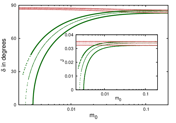
In the following $m_{0},\theta_{13}$, and $\theta_{12}$ are taken as inputs and $\delta$ and $\theta_{23}$ are obtained using eqs. (27) and (25). From these the CP-violation measure, $J$, and the combination $|m_{\nu_{e}\nu_{e}}|$ which determines the rate of neutrinoless double beta decay are calculated.

In the left panel of Fig. 2 is shown (thick curves) the dependence of $\theta_{23}$ on the lightest neutrino mass $m_{0}$ when the neutrino mass square splittings and the angles $\theta_{13}$ and $\theta_{12}$ are varied over their allowed ranges at 3$\sigma$. The thin curves correspond to taking the best-fit values. The green (pink) curves are for normal (inverted) mass ordering while solid (dashed) curves are for solutions in the first (second) octant. For inverted ordering the thick and thin curves are very close and cannot be distinguished in this figure. Notice that the 3$\sigma$ predictions from this model are not consistent with $\theta_{23}=\pi/4$. As expected from eq. (25), $\theta_{23}$ values are symmetrically distributed around $\pi/4$. Its range for inverted ordering falls outside the 1$\sigma$ global fits but are consistent at 3$\sigma$. An improvement in the determination of $\theta_{23}$ will be the easiest way to exclude one of the orderings unless one is in the quasidegenerate regime. For normal ordering the smallest value of $m_{0}$ is determined by the 3$\sigma$ limits of $\theta_{23}$ in the two octants. Eq. (26) permits arbitrarily small $m_{0}$ for inverted mass ordering (see below).

In the right panel of Fig. 2 $|m_{\nu_{e}\nu_{e}}|$ has been plotted. The sensitivity of direct neutrino mass measurements is expected to reach around 200 meV [7] in the near future. Planned neutrinoless double beta decay experiments will also probe the quasidegenerate range of $m_{0}$ [8]. As can be seen from this figure, to distinguish the two mass orderings at least a further one order improvement in sensitivity will be needed. Long baseline experiments or large atmospheric neutrino detectors such as INO will settle the mass ordering more readily.

In Fig. 3 is displayed the variation of $\delta$ with $m_{0}$ for both mass orderings while $J$ is shown in the inset. The conventions are the same as in Fig. 2. The sign of $J$ is positive if $\delta$ is in the first or second quadrant and is negative for the other cases. As noted, the quadrant of $\delta$ (and the associated sign of $J$) can be altered by the choice of the quadrant of $\phi_{1}$. However, from eq. (27) for these alternatives, namely, $\pm\delta$ and $(\pi\pm\delta)$, the dependence of $|\cos\delta|$ on $m_{0}$ is the same for a particular mass ordering. With this proviso in mind, Fig. 3 has been plotted keeping $\delta$ in the first quadrant and $J$ has been taken as positive.

$J$, which is proportional to $\sin 2\theta_{23}$, has no dependence on the octant of $\theta_{23}$ as the latter is symmetrical around $\pi/4$. In both Figs. 2 and 3, for normal ordering a slightly larger range of $m_{0}$ is allowed when $\theta_{23}$ is in the second octant. For the region where both octants are allowed the curves in Fig. 3 completely overlap. For inverted mass ordering both $\delta$ and $J$ remain nearly independent of $m_{0}$.

For $m_{0}$ smaller than 10 meV, the CP-phase $\delta$ is significantly larger for inverted ordering⁵⁵ 5 In fact for inverted ordering $\delta$ remains close to $\pi/2$ or $3\pi/2$ for all $m_{0}$.. This could provide a clear test of this model when the mass ordering is known and CP-violation in the neutrino sector is measured. The real limit ($\delta$ = 0) is seen to be admissible, as expected from Fig. 1, only for normal ordering and that too not for the entire 3$\sigma$ range, with the second octant allowing a larger region.

Since $0\leq z\leq 1/2$ for NO and $1/2\leq z\leq 1$ for IO, the allowed values of $\delta$ in the two orderings as seen from eq. (27) are complementary tending towards a common value as $z\rightarrow 1/2$, the quasidegenerate limit, which begins to set in from around $m_{0}$ = 100 meV. The main novelty from the real $M_{R}$ case is that in eq. (15) by choosing $\cos\delta$ sufficiently small one can make $z\equiv m^{-}m^{(0)}_{1}/\Delta m^{2}_{atm}\sim 1$ so that solutions exist for $m_{0}$ for inverted mass ordering corresponding to even vanishing $m_{0}$ unlike the case of normal ordering where the lower limit of $m_{0}$ is set by $\cos\delta=1$, i.e., real $M_{R}$.

We have checked that the size of the perturbation is at most around 20% of the unperturbed contribution for all cases.

In conclusion, a model for neutrino masses has been proposed in which the atmospheric mass splitting together with $\theta_{23}=\pi/4$ has an origin different from that of the solar mass splitting, $\theta_{12}$, $\theta_{13}$, and $\omega=\pi/4-\theta_{23}$, all of which arise from a single perturbation resulting from a Type-I see-saw. The global fits to the mass splittings, $\theta_{12}$ and $\theta_{13}$ completely pin-down the model and the CP-phase $\delta$ and the octant of $\theta_{23}$ are predicted in terms of the lightest neutrino mass $m_{0}$. Both mass orderings are allowed, the inverted ordering being associated with near-maximal CP-violation. Both octants of $\theta_{23}$ can be accommodated. Further improvements in the determination of $\theta_{23}$, a measurement of the CP-phase $\delta$, along with a knowledge of the neutrino mass ordering will put this model to tests from several directions.

Acknowledgements: SP acknowledges a Senior Research Fellowship from CSIR, India. AR is partially funded by the Department of Science and Technology Grant No. SR/S2/JCB-14/2009.

References

- [1] For the present status of see presentations from Double Chooz, RENO, Daya Bay, MINOS/MINOS+ and T2K at Neutrino 2014. https://indico.fnal.gov/conferenceOtherViews.py?view=standard&confId=8022.
- [2] M. C. Gonzalez-Garcia, M. Maltoni, J. Salvado and T. Schwetz, JHEP 1212, 123 (2012) [arXiv:1209.3023v3 [hep-ph]], NuFIT 1.3 (2014).
- [3] D. V. Forero, M. Tortola and J. W. F. Valle, Phys. Rev. D 86, 073012 (2012) [arXiv:1205.4018 [hep-ph]].
- [4] P. Minkowski, Phys. Lett. B 67, 421 (1977); M. Gell-Mann, P. Ramond and R. Slansky, in Supergravity, p. 315, edited by F. van Nieuwenhuizen and D. Freedman, North Holland, Amsterdam, (1979); T. Yanagida, Proc. of the Workshop on Unified Theory and the Baryon Number of the Universe, KEK, Japan, (1979); S.L. Glashow, NATO Sci. Ser. B 59, 687 (1980); R.N. Mohapatra and G. Senjanović, Phys. Rev. D 23, 165 (1981).
- [5] Earlier work on neutrino mass models in which a few elements dominate over others can be traced to F. Vissani, JHEP 9811, 025 (1998) [hep-ph/9810435]. Models with somewhat similar points of view as those espoused here are E. K. Akhmedov, Phys. Lett. B 467, 95 (1999) [hep-ph/9909217], and M. Lindner and W. Rodejohann, JHEP 0705, 089 (2007) [hep-ph/0703171].
- [6] For more recent work after the determination of see, for example, B. Brahmachari and A. Raychaudhuri, Phys. Rev. D 86, 051302 (2012) [arXiv:1204.5619 [hep-ph]]; B. Adhikary, A. Ghosal and P. Roy, Int. J. Mod. Phys. A 28, 1350118 (2013) arXiv:1210.5328 [hep-ph]; D. Aristizabal Sierra, I. de Medeiros Varzielas and E. Houet, Phys. Rev. D 87, 093009 (2013) [arXiv:1302.6499 [hep-ph]]; R. Dutta, U. Ch, A. K. Giri and N. Sahu, Int. J. Mod. Phys. A 29, 1450113 (2014) arXiv:1303.3357 [hep-ph]; L. J. Hall and G. G. Ross, JHEP 1311, 091 (2013) arXiv:1303.6962 [hep-ph]; T. Araki, PTEP 2013, 103B02 (2013) arXiv:1305.0248 [hep-ph]; M. -C. Chen, J. Huang, K. T. Mahanthappa and A. M. Wijangco, JHEP 1310, 112 (2013) [arXiv:1307.7711] [hep-ph]. S. Pramanick and A. Raychaudhuri, Phys. Rev. D 88, 093009 (2013) [arXiv:1308.1445 [hep-ph]]; B. Brahmachari and P. Roy, JHEP 1502, 135 (2015) [arXiv:1407.5293 [hep-ph]].
- [7] M. Haag [KATRIN Collaboration], PoS EPS -HEP2013, 518 (2013).
- [8] W. Rodejohann, Int. J. Mod. Phys. E 20, 1833 (2011) [arXiv:1106.1334 [hep-ph]].
Abstract
Neutrino oscillations reveal several small parameters, namely, , the solar mass splitting vis-à-vis the atmospheric one, and the deviation of from maximal mixing. Can these small quantities all be traced to a single source and, if so, how could that be tested? Here a see-saw model for neutrino masses is presented wherein a dominant term generates the atmospheric mass splitting with maximal mixing in this sector, keeping and zero solar splitting. A Type-I see-saw perturbative contribution results in non-zero values of , , , as well as allows to deviate from in consistency with the data while interrelating them all. CP-violation is a natural consequence and is large () for inverted mass ordering. The model will be tested as precision on the neutrino parameters is sharpened.
Key Words: Neutrino mixing, , Leptonic CP-violation, Neutrino Mass ordering, Perturbation