Fluctuation-induced Nambu-Goldstone bosons in a Higgs-Josephson model

Introduction When global and continuous symmetries are spontaneously broken, gapless excitation modes, called the Nambu-Goldstone bosons, exist and govern the long-distance behaviors of the system[1, 2, 3]. When the $U(1)$ rotational symmetry is spontaneously broken, there is a massless Nambu-Goldstone boson. When there is an interaction that violates the $U(1)$ symmetry, we have no massless boson. An interesting question is whether such an interaction will continuously conceal the Nambu-Goldstone bosons when the perturbative corrections are taken into account. We present a model that exhibits a fluctuation induced Nambu-Goldstone boson in this paper. This means that a massless boson appears inspite of an interaction that hides Nambu-Goldstone bosons. We propose the mechanism of fluctuation induced Nambu-Goldstone boson.

We consider a model of an n-component scalar field with Josephson interactions, so called the Higgs-Josephson model[4, 5, 6, 7]. Let us consider the action given as

where $\phi\equiv(\phi_{1},\cdots,\phi_{n})$ is a complex n-component scalar field. We write $\phi_{j}$ as

where $\rho_{j}$ ($j=1,\cdots,n$) are real scalar fields. The last term in the action is the Josephson term. We assume that $\gamma_{ij}$ are real and $\gamma_{ij}=\gamma_{ji}$. Without this interaction, the phase modes $\theta_{j}$ $(j=1,\cdots,n)$ represent massless modes. Because of this term, we have $n-1$ phase massive modes and one massless mode as shown by expanding $\cos(\theta_{i}-\theta_{j})$ in terms of $\theta_{i}-\theta_{j}$. We adopt that $\beta_{j}$ is positive so that the action has a minimum. When $\alpha_{j}$ is negative, $\rho_{j}$ takes a finite value at the minimum of the potential. We set this value as $\Delta_{j}$ and write $\rho_{j}=\Delta_{j}+H_{j}$. $H_{j}$ is the Higgs field and represents fluctuation of the scalar field around the minimum $\Delta_{j}$. We simply assume that $K=K_{j}$, $\Delta=\Delta_{j}$ and $\gamma_{ij}=\gamma_{ji}\equiv\gamma$. Then the action for the phase variables $\theta_{j}$ is

where $t/\Lambda^{d-2}=k_{B}T/(K\Delta^{2})$ and $\lambda\Lambda^{2}=\gamma/K$. We have introduced the cutoff $\Lambda$ so that $t$ and $\lambda$ are dimensionless parameters. We assume that $\lambda>0$ in this paper. We now focus on $\theta_{j}$ and consider the case $n=3$. Since the potential term is written as

the mode of the total phase $\theta_{1}+\theta_{2}+\theta_{3}$ remains massless. We do not consider this mode because the coupling to the gauge field turns this mode into a gapped mode (Higgs mechanism). The other $n-1$ modes do not become massive by the coupling to the gauge field. Let us consider the case $\lambda>0$. As is easily shown, the ground state of $V$ has a $2\pi/3$ structure, namely, $\theta_{2}-\theta_{1}=2\pi/3$ and $\theta_{3}-\theta_{2}=2\pi/3$ as shown in Fig.1(a). The state in Fig.1(b) has also the same energy. Two states are indexed by the chirality $\kappa=1$ for (a) and $\kappa=-1$ for (b), where $\kappa$ is defined by $\kappa=(2/3\sqrt{3})(\sin(\theta_{2}-\theta_{1})+\sin(\theta_{3}-\theta_{2})+\sin(\theta_{1}-\theta_{3})$[8, 9, 10, 11, 12, 13, 14, 15]. We set $\varphi_{1}=\theta_{3}-\theta_{1}$ and $\varphi_{2}=\theta_{1}-2\theta_{2}+\theta_{3}$ to write the potential density as

$V$ has a minimum at $\varphi_{1}=4\pi/3$ and $\varphi_{2}=0$. We mention here that an $S_{3}$ symmetry of the Josephson potential is not lost when we express the potential in terms of $\varphi_{1}$ and $\varphi_{2}$. When $V$ has a minimum at some value of $\varphi_{1}=\theta_{3}-\theta_{1}$, $V$ has also a minimum when $\theta_{3}-\theta_{2}$ takes the same value (modulo $2\pi$). When the former has the chirality $\kappa=1$, the latter has $\kappa=-1$. We consider the fluctuation around this minimum. For this purpose, we perform a unitary transformation by defining $\varphi_{1}=4\pi/3+\sqrt{2}\eta_{1}$ and $\varphi_{2}=\sqrt{6}\eta_{2}$:

where $\eta_{i}$ ($i=1,2,3$) indicate fluctuation fields. $\eta_{3}$ describes the total phase mode, $\eta_{3}=(\theta_{1}+\theta_{2}+\theta_{3})/\sqrt{3}$, and is not important in this paper because this mode turns out to be a plasma mode by coupling with the long-range Coulomb potential. We obtain $\sum_{i}(\nabla\theta_{i})^{2}=\sum_{i}(\nabla\eta_{i})^{2}$, and then the action $S[\eta]\equiv S[\theta]$ is

The potential term has a minimum at $\eta_{1}=\eta_{2}=0$. Both of $\eta_{1}$ and $\eta_{2}$ represent massive modes with mass $3\lambda/(2t)$.

Fluctuation induced Nambu-Goldstone boson The potential $V$ corresponds to the potential of a two-dimensional XY model on the triangular lattice with a frustrated interaction. The ground state has an well known $2\pi/3$-structure. We consider the role of fluctuation and show the existence of fluctuation-induced massless mode. We examine the following free-energy density by neglecting the kinetic term:

The partition function is given by

for the free energy functional $F$. Using the formula for the modified Bessel function,

we have, by using $\varphi_{2}/2=\sqrt{3/2}\eta_{2}$,

We use $I_{0}(-x)=I_{0}(x)$ and the asymptotic formula $I_{0}(z)\sim e^{z}/\sqrt{2\pi z}$ ($z>0$) at low temperature. Then the effective free-energy density for $\eta_{1}$ is

where $\epsilon_{0}\equiv k_{B}T\lambda/t$. We have an effective entropy term being proportional to the temperature $T$. $F[\eta_{1}]$ has a minimum at $\eta_{1}=0$ ($\varphi_{1}=4\pi/3$) at absolute zero $T=0$. In contrast, at finite temperature $T>0$, the minimum is at $\eta_{1}=-\sqrt{2}\pi/6$ and $\varphi_{1}=\pi$. This is shown in Fig.2 where we present the potential $f[\eta_{1}]/\epsilon_{0}$ as a function of $\varphi\equiv\varphi_{1}=4\pi/3+\sqrt{2}\eta_{1}$ for $t=\lambda$ with setting $\Lambda=1$. At $\varphi=\pi$, $\eta_{2}$ becomes a massless boson because the free-energy density in eq.(10) becomes independent of $\eta_{2}$ with vanishing of the mass term. This is due to the fluctuation of $\eta_{2}$ field at finite temperature. The qualitatively same result is obtained by the Gaussian integration with respect to $\eta_{2}$ after expanding cosine function as $\cos(\sqrt{3/2}\eta_{2})=1-(3/4)\eta_{2}^{2}+\cdots$ and assuming that $\cos(\eta_{1}/\sqrt{2}+2\pi/3)<0$. (We can use the formula $I_{0}(z)\sim e^{z}/\sqrt{2\pi z}$ when $z>0$ is large. In the limit $z\rightarrow 0$, we have a largee entropy coming from the volume of the phase space and thus the minimum is at $\varphi_{1}=\pi$ for $T>0$ when $T$ is higher than a critical value.) This state is shown in Fig.1(c) using a spin analogue where we have two antiferromagnetic spins and one vanishing spin. This means that the $\eta_{2}$-mode is massless and $\varphi_{2}=\sqrt{6}\eta_{2}=\theta_{1}-2\theta_{2}+\theta_{3}$ can take any value. At the absolute zero, we have the index of chirality $\kappa=\pm 1$ as shown in Figs.1(a) and 1(b). The chirality disappears at finite temperature leading to the emergency of a Nambu-Goldstone boson. This represents a phenomenon that the Nambu-Goldstone boson appears due to a fluctuation effect.

Phase transition at finite temperature We next consider the kinetic terms of $\eta_{j}$. For this purpose, we use the expansion of cosine term and write the action in the form

When $\cos(\varphi_{1}/2)<0$, we use $\cos(\sqrt{3/2}\eta_{2})=1-(4/3)\eta_{2}^{2}+\cdots$. Around the minimum at $\varphi_{1}=2\pi/3$ and $\varphi_{2}=2\pi$ (with chirality $\kappa=-1$), we use instead the expansion by defining $\varphi_{2}=2\pi+\sqrt{6}\eta_{2}$. We integrate out the field $\eta_{2}$ to obtain the effective action, using $\varphi\equiv\varphi_{1}=4\pi/3+\sqrt{2}\eta_{1}$,

When we neglect the kinetic term $-\nabla^{2}$, this action is reduced to the previous effective free energy. We adopt that the spatial variation of $\varphi$ field is very slow so that we can perform the ${\bf k}$-summation for $-\nabla^{2}={\bf k}^{2}$. In the two-dimensional case $(d=2)$, the effective free-energy density is obtained as

where we have chosen the cutoff $k_{0}$ in the momentum space as $k_{0}^{2}=c\Lambda^{2}$ for a constant $c$.

The spatial fluctuation softens the thermal fluctuation effect and there is a finite critical temperature where the minimum at $\varphi=4\pi/3$ disappears and simultaneously the chirality vanishes. We show the potential term as a function of $\varphi$ for $t=2c$ and $\lambda=c$ with $c=4\pi$ in Fig.3 where we subtracted the term $k_{B}T/2\ln\Lambda^{d}$ which is independent of $\varphi$ (or equivalently we set $\Lambda=1$). We have a minimum at $\varphi=\pi$ when $t$ is large as shown in Fig.3. The critical temperature $t_{c}$ is scaled by $\lambda/c$:

$t_{c}$ is estimated by the equation $V(\varphi=4\pi/3)=V(\varphi=\pi)$, which gives

For small $\lambda\rightarrow 0$, $t_{c}$ is small: $t_{c}\simeq 16\pi/(3\ln(1/3\lambda))$. When $\lambda$ is large, $\lambda\gg 1$, $t_{c}$ is also large $t_{c}\simeq 4\pi\lambda/c\ln(3\lambda/4c)$. In Fig.4 we show the potential for $t/c=0.5$, $0.935$, $2$, and $\lambda/c=1$ with $c=4\pi$. When $t$ is small, the potential has a minimum at $\varphi=4\pi/3$ or at $\varphi=2\pi/3$ indicating that the ground state has the $2\pi/3$ structure with the chirality $\pm 1$. In contrast, when $t$ is large, we have a minimum $\varphi=\pi$. There is a transition at finite temperature $t=t_{c}$. This is a first-order transition since we have the double-minimum potential in the range $\pi\leq\varphi\leq 2\pi$. This should be called a weak first-order transition because the change of $V_{total}(\varphi=\pi)$ is slow as $t$ is varied near the critical temperature. The minimum point of $\varphi$ changes gradually from $4\pi/3$ and changes suddenly to $\pi$ at the critical temperature. For $t>t_{c}$, the $\eta_{2}$-mode represents a massless boson. We show $t_{c}$ as a function of $\lambda/c$ in Fig.5.

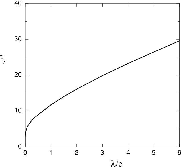
We discuss a relation to the classical XY model on a two-dimensional triangular lattice. The ground state of the 2D XY model has the $2\pi/3$-structure to minimize the energy. There is a transition of the chirality at finite temperature. The critical temperature $T_{c}$ is of the order of the exchange coupling $J$ because $\lambda/t=J/k_{B}T$ in this case. The Kosterlitz-Thouless (KT) transition also occurs in the XY model on the 2D triangular lattice. The critical temperature of the KT transition $T_{KT}$ is determined by the renormalization group equation. In general, $T_{KT}$ is different from the critical temperature of the chiral transition $T_{chiral}\equiv K\Delta^{2}t_{c}$.

The similar phenomenon occurs for an $n=4$ theory with the potential

where $a\geq 1$ is a constant. This model has a close relation with the 2D antiferromagnetic XY model on a square lattice[16, 17]. One of the ground state is given by $(\theta_{1},\theta_{2},\theta_{3},\theta_{4})=(0,\theta,\pi,\theta+\pi)$ where real $\theta$ is arbitrary and the ground state is degenerate with respect to $\theta$. We define $\varphi_{1}=\theta_{1}-\theta_{2}-\theta_{3}+\theta_{4}=\eta_{1}$, $\varphi_{2}=\theta_{1}+\theta_{2}-\theta_{3}-\theta_{4}=\eta_{2}-2\pi$, $\varphi_{3}=\theta_{1}-\theta_{2}+\theta_{3}-\theta_{4}=\eta_{3}-2\theta$, and the total phase $\Phi=\theta_{1}+\theta_{2}+\theta_{3}+\theta_{4}$. Then the potential becomes

where $\cdots$ indicates higher order terms. The $\eta_{3}$-mode becomes massless and the ground state energy $-2a$ is independent of $\theta$. This is the $n-3$ series state[18] which we call the type I. When $a=1$, $\eta_{1}$- or $\eta_{2}$-mode is massless in the case $\theta=0$ or $\pi$. This is the $n-2$ series state. The effective potential $V_{eff}$ is obtained by integrating out the $\eta_{1}$ and $\eta_{2}$ variables in a similar way to the case $n=3$ in two dimensions:

where we used the cutoff $k_{0}$ in the momentum integral satisfying $k_{0}^{2}/(4\pi)=\Lambda^{2}$. The potential is shown in Fig.6 for several parameters where the ground state is at $\theta=m\pi$ for an integer $m$. This indicates that a Nambu-Goldstone boson emerges for $a=1$ as a result of fluctuation of the $U(1)$ phase variables. We can regard the sign of $\sin\theta$ as a kind of chirality. The emergence of new massless boson is accompanied by the vanishing of chirality.

We can generalize our argument to an $n$-component scalar field with Josephson couplings. The potential

has a series of massless bosons; there are two types of ground states called the type I and II[18]. In the ground state I one has $n-3$ massless bosons and in the ground state II one has $n-2$ massless bosons. (The $n-2$ series exists only for even $n$.) Two ground states I and II are degenerate for the potential $V$. However, the ground state II becomes more stable than the state I due to fluctuation effect. Thus, when we are in the ground state I first, the fluctuation effect leads us to the state II with increasing the number of Nambu-Goldstone bosons.

Order to order transition by disorder The chiral transition considered in this paper is a transition from the $2\pi/3$-structure in Fig.1(a) (or (b)) to the antiferromagnetic state in Fig.1(c). We can say that the ordered state with a massless boson in Fig.1(c) is induced by disorder, namely, thermal fluctuation. We call this an order to order transition by disorder. We discuss here the fluctuation effect on the induced Nambu-Goldstone boson. For this purpose, we write $\varphi_{1}=\pi+\phi_{1}$ so that $\phi_{1}$ indicates the fluctuation mode in the neighborhood of $\pi$. The action is written as

The $\varphi_{2}$-mode is obviously a massless mode, but there is an interaction with $\phi_{1}$. This interaction will generate an effective potential of $\varphi_{2}$ that is proportional to $\cos^{2}(\varphi_{2}/2)=(\cos(\varphi_{2})+1)/2$. Then, the effective action for $\varphi_{2}$ is given by the sine-Gordon model:

The low-energy property is determined by the values of $\lambda$ and $t$ as indicated by the renormalization group equations[26, 27] near two dimensions. The critical value of $t$, denoted by $t_{2c}$, is $t_{2c}=8\pi/3$. We assume that $t>t_{c}>t_{2c}$. When $\lambda$ is small, $\lambda$ is renormalized to $0$ following the renormalization flow. This indicates that the $\varphi_{2}$-mode remains massless for small $\lambda$. When $\lambda$ is large, $\lambda$ is renormalized to be a large value, showing that the potential term dominates the behavior of $\varphi_{2}$-mode and then that $\varphi_{2}$ takes the value near $0$. In this case the massless $\varphi_{2}$-mode becomes massive, that is, a gapped mode again. Basically $\varphi_{2}$-mode may remain massless because the Josephson coupling $\lambda$ is small in real superconductors.

Summary We have proposed the mechanism of fluctuation induced Nambu-Goldstone bosons. In an n-component scalar field theory with frustrated Josephson interactions, massless bosons appear due to fluctuations at finite temperature. In the 3-component theory discussed in the paper, a massless boson appears and the chirality vanishes as the temperature is increased, that is, the $Z_{2}$-symmetry breaking is driven by the chirality. This shows that nature prefers massless bosons. In fact, in an n-component model, the ground state at absolute zero will flow into the state with more massless bosons as the temperature is increased from $(n-3)$-state to $(n-2)$-state.

The excitation modes in our model has an analogy to the vibration modes of a molecule CH₂. Two modes, the scissoring mode and the rocking mode, are important in determining the excitation spectra of CH₂[28, 29]. The modes shown by $\varphi_{1}=\theta_{3}-\theta_{1}$ and $\varphi_{2}=\theta_{1}-2\theta_{2}+\theta_{3}$ represent the scissoring and rocking modes, respectively. In our model, the rocking mode plays a significant role. The fluctuation effect of the rocking mode becomes large as the temperature is increased and gives rise to the phase transition. The model presented in the paper appears as an effective free energy in multi-band superconductors[13, 14, 15, 19, 20, 21, 22, 23]. Low energy excitation states are important in superconductors, the existence of massless modes have been pointed out[18, 21, 24, 25]. In this paper we have presented a new mechanism of the emergence of Nambu-Goldstone bosons.

We express our sincere thanks to J. Kondo and I. Hase for useful discussions. This work was supported by a Grant-in-Aid for Scientific Research from the Ministry of Education, Culture, Sports, Science and Technology of Japan.

References

- [1] Y. Nambu, Phys. Rev. 117, 648 (1960).
- [2] Y. Nambu, Broken Symmetry Selected Papers of Y. Nambu, edited by T. Eguchi and K. Nishijima, World Scientific, Singapore 1995.
- [3] J. Goldstone, Nuovo Cimento 19, 154 (1961).
- [4] P. W. Higgs, Phys. Rev. Lett. 13, 508 (1964).
- [5] P. W. Higgs, Phys. Rev. 145, 1156 (1966).
- [6] B. D. Josephson, Rev. Lett. 1, 251 (1962).
- [7] B. D. Josephson, Rev. Mod. Phys. 36, 216 (1964).
- [8] S. Miyashita and H. Shiba, J. Phys. Soc. Jpn. 53, 1145 (1984).
- [9] Y. Ozeki and N. Ito, Phys. Rev. B68, 054414 (2003).
- [10] M. Hasenbusch and A. Peliseto and E. Vicati, J. Stat. Mech. P12002 (2005).
- [11] S. Okumura, H. Yoshino and H. Kawamura, Phys. Rev. B83, 094429 (2011).
- [12] T. Obuchi and H. Kawamura, J. Phys. Soc. Jpn. 81, 054003 (2012).
- [13] Y. Tanaka and T. Yanagisawa, J. Phys. Soc. Jpn. 79, 114706 (2010).
- [14] Y. Tanaka and T. Yanagisawa, Solid State Commun. 150, 1980 (2010).
- [15] T. Yanagisawa, Y. Tanaka, I. Hase and K. Yamaji, J. Phys. Soc. Jpn. 81, 024712 (2012).
- [16] C. L. Henley, Phys. Rev. Lett. 62, 2056 (1989).
- [17] D. Loison and P. Simon, Phys. Rev. B61, 6114 (2000).
- [18] T. Yanagisawa and I. Hase, J. Phys. Soc. Jpn. 82, 124704 (2013).
- [19] V. Stanev and Z. Tesanovic, Phys. Rev. B81, 134522 (2010).
- [20] R. G. Dias and A. M. Marques, Supercond. Sci. Technol. 24, 085009 (2011).
- [21] S.-Z. Lin and X. Hu, Phys. Rev. Lett. 108, 177005 (2012).
- [22] B. J. Wilson and M. P. Das, J. Phys.: Condens. Matter 25, 425702 (2013).
- [23] S. Malti and A. V. Chubukov, Phys. Rev. B87, 144511 (2013).
- [24] K. Kobayashi, M. Machida, Y. Ota and F. Nori, Phys. Rev. B88, 224516 (2013).
- [25] Y. Tanaka, T. Yanagisawa, A. Crisan, P. M. Shirage, A. Iyo, K. Tokiwa, T. Nishio, A. Sundaresan and N. Terada, Physica C471, 747 (2011).
- [26] D. J. Amit, Y. Y. Goldschmidt and G. Grinstein, J. Phys. A13, 585 (1980).
- [27] J. Zinn-Justin, Quantum Field Theory and Critical Phenomena (Oxford University Press, Oxford, 2002).
- [28] T. J. Sears, R. R. Bunker, A. R. W. McKellar, K. M. Evenson, D. A. Jennings and J. M. Brown: J. Chem. Phys. 77, 5348 (1982).
- [29] D. G. Leopold, K. K. Murray and W. C. Lineberger: J. Chem. Phys. 81, 1048 (1984).