Velocity-density twin transforms in thin disk model

In this paper we deal with axisymmetric and infinitesimally thin disk model. We use cylindrical coordinate system $\rho,\phi,z$.

Given a surface mass density $\sigma(\rho)$ in the disk plane $z=0$, we can infer the circular velocity $v(\rho)$ of test bodies moving in that plane. Conversely, given a $v(\rho)$, we can find the corresponding $\sigma(\rho)$. Instead of $\sigma(\rho)$ it is more convenient to consider the ring density $\mu(\rho)=2\pi G\,\rho\,\sigma(\rho)$. In the next section we show that

• The quantities $\mu(\rho)$ and $v^{2}(\rho)$ are related through the following pair of mutually inverse integral expressions with the same weighting function $w(x)$:

The one-fold integral forms are more suitable for numerical integration than the equivalent double-integral (or chain forms) which we shall come to later.

The weighting function $w(x)$ in both integrals is given by a combination of complete elliptic integrals $K$ and $E$:¹¹ 1 We use $K$ and $E$ as defined by Gradshtein et al. (2007)

Because $w(x)$ has an integrable singularity at $x=1$, the integration should be understood in the Cauchy principal value sense. The nature of the pole $x=1$ is such that the integrals are sensitive to the radial gradients of the integrands $\mu$ and $v^{2}$. This is a characteristic feature of the disk model.

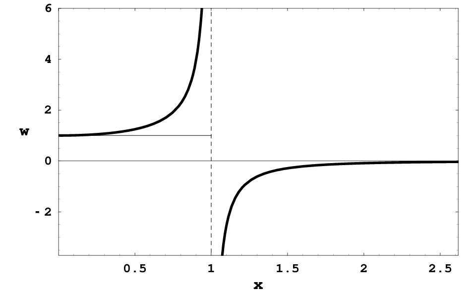
Despite the wide use of disk model, it seems that Eq.2 may not be widely known. A more familiar is the equivalent Toomre (1963) integrated formula

which contains only a logarithmic singularity of $K$, but on the cost of involving the derivative of $v^{2}$ which introduces additional uncertainty in modeling galactic disks. The usual advice about numerical evaluation of singular integrals is to integrate by parts, which may be the reason why Toomre (1963) gave no expression in form of a one-fold integral without the derivative of $v^{2}$. But the singularity in $w(x)$ is nowadays easily tractable numerically and presents itself no difficulty at all.

A word of warning may be appropriate, here. Owing to the sensitivity to radial gradients mentioned above, the disk model was pointed out in the context of Toomre’s integrated formula to be of relatively little use in practice on account of the fact that the derivative of $v^{2}$ is usually subject to significant observational errors, resulting in a $\sigma$ varying in an erratic and unphysical way (Binney & Tremaine, 1987). The disk model has also other limitations. In realistic situations the rotation curves do not extend far enough and one has to extrapolate the data. Unfortunately, the results depend on the way one choses to extrapolate. Therefore, the disk model must be used with due care.

We decided to focus on the integral form Eq.2 in this separate paper, because of usefulness of a formula turning the rotation curve to the surface density in modeling galactic disks. A reduced one-fold integral form is needed for practical reasons, for the accuracy and speeding up the numerical integration, especially in finding column mass densities of finite-width disks by means of recursions, like in (Jałocha et al., 2014).

There are also known various forms of equivalent double integral representations of Eq.2, e.g. (Shatskiy et al., 2012) or those implied by Toomre (1963) or Kalnajs (1999) methods which we focus later on. We recall also that there are numerical methods of finding $\sigma$ from a fragment of $v^{2}$, given some other measurements complementary to the rotation data (Jałocha et al., 2008). An algebraic approach to inverting Eq.1 presented by Feng & Gallo (2011), offers an interesting alternative to the direct formula Eq.2 represented on a union of osculating rings, if it can be assumed that $\sigma$ practically vanishes beyond the last measured point of $v$. With transforms Eq.1 and Eq.2 cut-off at the last point, the same result can be then obtained by iterations, analogous to those in (Jałocha et al., 2008), assuming vanishing density beyond the cutoff.

Surface density for axi-symmetric discs is naturally expressed in terms of Hankel transforms which are a special case of Fourier transforms involving circular symmetry. For our purposes we intentionally rewrite the result of Toomre (1963) method into the chain form corresponding to Eq.2

Toomre called it as too formal to be of any direct use and, having integrated by parts, gave his integrated formula as the final result. Nevertheless, the above form with Bessel functions is useful in finding analytical expressions for $\sigma$, given a $v^{2}$ (or vice versa), e.g. (Freeman, 1970).

To complete our derivation, it remains to determine $u(x)$. Instead of using tables of integrals, we can deduce $u(x)$ by comparing the previous expression for $v^{2}$ with one from a textbook calculation concerning the axisymmetric gravitational potential $\Phi(\rho,z)$ of a thin disk. First, we arrange the expression for $\Phi$ so as to isolate the elliptic function $K$ (for a fixed $\phi$ we make use of a new integration variable $\tilde{\phi}\to\gamma$: $2\gamma=\tilde{\phi}-\phi+\pi$)

By differentiating $\Phi$ with respect to $\rho$, using the property $K^{\prime}(k)=\frac{E(k)}{k(1-k^{2})}-\frac{K(k)}{k}$ and taking the limit $z\to 0$, we can obtain the desired result from the force equilibrium condition $\rho^{-1}v^{2}(\rho)=\partial_{\rho}\Phi\left(\rho,0^{\pm}\right)$ for circular orbits in the disk plane. By substituting $\tilde{\rho}=\rho x$, and denoting $k(x)\equiv{2\sqrt{x}}/\left(1+x\right)$, the result can be simplified to

From this result we immediately see that $u(x)\equiv w(x)$, which in turn proves the relation Eq.2.²² 2 A similar expression to Eq.2 we obtained in a not so straightforward way in (Sikora et al., 2012) and it is connected with the present form by the inversion $x\to x^{-1}$.

There is a more sophisticated way of understanding the fact that the integrals turning $v^{2}$ to $\mu$ and $\mu$ to $v^{2}$ can be put into forms with the same weight function.

Kalnajs (1999) related column density $\sigma(\rho)$ to the circular velocity $v^{2}(\rho)$ in the plane $z=0$ for a spheroid with similar isodensity surfaces $\rho^{2}+z^{2}/q^{2}=m^{2}$ characterized by a fixed flattening $q$ and parameterized by $m$. With the definitions $\hat{P}(\alpha)\equiv\frac{\Gamma(3/2)\Gamma((1-i\alpha)/2)}{\Gamma(1-i\alpha/2)}$ and $\hat{S}(\alpha,q)\equiv\left(1+i\alpha\right)^{-1}\cdot{}_{2}F_{1}(1,1+i\alpha,(3+i\alpha)/2,(1-q)/2)$, Kalnajs’ result can be arranged in the chain form

Kalnajs’ method exploits the translational symmetry in the scale-invariant variable $u=\ln\left(\rho/\rho_{o}\right)$ ($\rho_{o}$ being an arbitrary and fixed scale parameter). For $q=0$ the ratio $\frac{\hat{S}(\alpha,q)}{\hat{P}(\alpha)}$ reduces to $\frac{\hat{P}(-\alpha)}{\hat{P}(\alpha)}$ with absolute value $1$. It then makes sense to consider the inverse convolution whose Fourier transform is $\frac{\hat{P}(\alpha)}{\hat{P}(-\alpha)}$.³³ 3 For nonzero flattening, the ratio $\frac{\hat{S}(\alpha,q)}{\hat{P}(\alpha)}$ tends to $0$ at infinity and we cannot write the inverse convolution form, the absolute value of that ratio only tends non-uniformly to $1$ as $q\to 0$. This allows us to write down the following integrals with identical weight functions

(in the second integral we have reflected the variables $\alpha,u,\tilde{u}$ with respect to $0$). The above expressions are counterparts of Toomre’s chain forms.

As a byproduct from the two methods we can deduce the following integral representations of function $w(x)$:

References

- Binney & Tremaine (1987) Binney J., Tremaine S., 1987, Galactic dynamics
- Bratek et al. (2008) Bratek Ł., Jałocha J., Kutschera M., 2008, MNRAS, 391, 1373
- Feng & Gallo (2011) Feng J. Q., Gallo C. F., 2011, Research in Astronomy and Astrophysics, 11, 1429
- Freeman (1970) Freeman K. C., 1970, ApJ, 160, 811
- Gradshtein et al. (2007) Gradshtein I., Ryzhik I., Jeffrey A., Zwillinger D., 2007, Table of integrals, series and products. Academic Press
- Jałocha et al. (2008) Jałocha J., Bratek Ł., Kutschera M., 2008, ApJ, 679, 373
- Jałocha et al. (2014) Jałocha J., Sikora S., Bratek Ł., Kutschera M., 2014, A&A, 566, A87
- Kalnajs (1999) Kalnajs A. J., 1999, in Gibson B. K., Axelrod R. S., Putman M. E., eds, The Third Stromlo Symposium: The Galactic Halo Vol. 165 of Astronomical Society of the Pacific Conference Series, Rotation Curves of Galaxies. p. 325
- Shatskiy et al. (2012) Shatskiy A. A., Novikov I. D., Silchenko O. K., Hansen J., Katkov I. Y., 2012, MNRAS, 420, 3071
- Sikora et al. (2012) Sikora S., Bratek Ł., Jałocha J., Kutschera M., 2012, A&A, 546, A126
- Toomre (1963) Toomre A., 1963, ApJ, 138, 385