Results from lattice simulations
of $\mathcal{N}=4$ supersymmetric Yang–Mills

The lattice theory we employ results from discretizing a topologically twisted form of continuum $\mathcal{N}=4$ SYM with gauge group SU($N$). There are three independent topological twists of $\mathcal{N}=4$ SYM, of which we employ the Marcus or Geometric-Langlands twist [15, 16]. This twisted theory is most conveniently written as a dimensional reduction of a five-dimensional action

$$S=\frac{N}{2\lambda}\mathcal{Q}\int d^{5}x\left(\chi_{ab}\mathcal{F}_{ab}+\eta\left[\overline{\mathcal{D}}_{a},\mathcal{D}_{a}\right]+\frac{1}{2}\eta d\right)-\frac{N}{8\lambda}\int d^{5}x\ \epsilon_{abcde}\ \chi_{ab}\overline{\mathcal{D}}_{c}\chi_{de}.$$

(1)

$\lambda=g^{2}N$ is the ’t Hooft coupling. The gauge fields $\mathcal{A}_{a}$ (and their associated covariant derivatives $\mathcal{D}_{a}$ and $\overline{\mathcal{D}}_{a}$) have real parts which are just the usual Yang–Mills gauge fields, while their imaginary parts arise from the five scalars that appear after reducing $\mathcal{N}=1$ SYM in ten dimensions down to five dimensions. The appearance of the scalar fields as vectors is odd at first sight, but is at the heart of the twisting process.

Twisting decomposes the fields under the diagonal subgroup of the Euclidean Lorentz symmetry and the R symmetry of the theory. Since the scalars transform as vectors under the R symmetry they remain vectors under the twisted symmetry, and naturally combine with the R-singlet gauge fields. Similar arguments show that twisting transforms the original four Majorana fermions into a set of antisymmetric fields with integer spins under the twisted symmetry, appearing as $(\eta,\psi_{a},\chi_{ab})$ in the above action. Likewise the $\mathcal{N}=4$ fermionic supercharges $Q_{\alpha i}$, $Q_{\dot{}\alpha i}^{{\dagger}}$ become integer-spin $(\mathcal{Q},\mathcal{Q}_{a},\mathcal{Q}_{ab})$. In flat space twisting does not change the physical content of the theory. It is merely an exotic change of variables, to a spinor-free form better suited to discretization.

The first part of the action in Eq. 1 is the $\mathcal{Q}$ variation of a function. This scalar supercharge $\mathcal{Q}$ is the supersymmetry that can be preserved under discretization. It acts on the fields as follows:

		$\displaystyle\mathcal{Q}\;\mathcal{A}_{a}=\psi_{a}$		$\displaystyle\mathcal{Q}\;\psi_{a}=0$		(2)
		$\displaystyle\mathcal{Q}\;\chi_{ab}=-\overline{\mathcal{F}}_{ab}$		$\displaystyle\mathcal{Q}\;\overline{\mathcal{A}}_{a}=0$		(3)
		$\displaystyle\mathcal{Q}\;\eta=d$		$\displaystyle\mathcal{Q}\;d=0.$

Its nilpotent character guarantees that the first piece of the action is trivially $\mathcal{Q}$ invariant. The second term can be shown to be invariant using the Bianchi identity, so that $\mathcal{Q}S=0$.

We recover the standard Marcus twist of four-dimensional $\mathcal{N}=4$ SYM from naive dimensional reduction, by simply setting to zero the momentum in the fifth dimension, $\partial_{4}=0$, and identifying the corresponding component of the gauge field as the sixth scalar field, $\mathcal{A}_{4}\to\phi$. A more symmetric choice is to project the theory onto the four-dimensional hyperplane with normal vector $\widehat{\mathbf{n}}=\frac{1}{\sqrt{5}}(1,1,1,1,1)$. This corresponds to setting $\sum_{a=0}^{4}\partial_{a}=0$ and $\sum_{a=0}^{4}\mathcal{A}_{a}\to\phi$, preserving an $S_{5}$ permutation symmetry.

Using this formalism, the transition to the lattice is quite straightforward. The lattice structure follows from a similar dimensional reduction. Starting with the five-dimensional hypercubic lattice in momentum space, the constraint $\sum_{a=0}^{4}\partial_{a}=0\to\sum_{a=0}^{4}n_{a}=0$ produces the $A_{4}$ lattice. Transforming back to real space leaves us with the dual $A_{4}^{*}$ lattice, which retains an $S_{5}$ point group symmetry manifest as five (linearly dependent) basis vectors symmetrically spanning four space-time dimensions. This $S_{5}$ symmetry provides a set of irreducible representations that match those of the continuum twisted SO(4) symmetry [17]. It can be useful to think of $A_{4}^{*}$ as the four-dimensional analog of the triangular lattice $A_{2}^{*}$ in two dimensions, or as the weight lattice of SU(5).

The complex gauge fields $\mathcal{A}_{a}(x)$ become complexified $\mathcal{U}_{a}(n)$ living on the five links of the $A_{4}^{*}$ lattice. The form of the nilpotent scalar supersymmetry $\mathcal{Q}$ remains the same as in the continuum (Eq. 3), and requires that these $\mathcal{U}_{a}(n)$ be elements of the algebra $\mathfrak{gl}(N,\mathbb{C})$, with consequences we will discuss in Section 3. Supersymmetry also forces us to assign the $\psi_{a}$ fermions to the same links, while the $\eta$ fermion and bosonic auxiliary field $d$ are placed on sites. The $\chi_{ab}$ fermions are associated with the field strengths

$$\overline{\mathcal{F}}_{ab}(n)=\overline{\mathcal{U}}_{a}(n+\widehat{\mu}_{b})\overline{\mathcal{U}}_{b}(n)-\overline{\mathcal{U}}_{b}(n+\widehat{\mu}_{a})\overline{\mathcal{U}}_{a}(n),$$

and connect lattice sites $n+\widehat{\mu}_{a}+\widehat{\mu}_{b}$ and $n$ so that their contractions with

$$\mathcal{D}_{a}^{(+)}\psi_{b}=\mathcal{U}_{a}(n)\psi_{b}(n+\widehat{\mu}_{a})-\psi_{b}(n)\mathcal{U}_{a}(n+\widehat{\mu}_{b})$$

will produce gauge invariant loops. After integrating out the auxiliary field $d$, on the lattice the two terms in Eq. 1 become

	$\displaystyle S_{exact}$	$\displaystyle=\frac{N}{2\lambda_{\rm lat}}\sum_{n}a^{4}\ \mbox{Tr}\left[-\overline{\mathcal{F}}_{ab}\mathcal{F}_{ab}(n)+\frac{1}{2}\left(\overline{\mathcal{D}}_{a}^{(-)}\mathcal{U}_{a}(n)\right)^{2}-\chi_{ab}\mathcal{D}_{[a}^{(+)}\psi_{b]}^{\ }(n)-\eta\overline{\mathcal{D}}^{(-)}_{a}\psi_{a}(n)\right]$
	$\displaystyle S_{closed}$	$\displaystyle=-\frac{N}{8\lambda_{\rm lat}}\sum_{n}a^{4}\ \mbox{Tr}\left[\epsilon_{abcde}\ \chi_{de}(n+\widehat{\mu}_{a}+\widehat{\mu}_{b}+\widehat{\mu}_{c})\overline{\mathcal{D}}^{(-)}_{c}\chi_{ab}(n)\right],$		(4)

where the specific form of the forward and backward difference operators can be found in Ref. [12].

This exactly supersymmetric lattice action was studied analytically in Refs. [9, 11, 13]. These studies have found that the single exact supersymmetry suffices to establish the following results:

• •

  The moduli space survives to all orders of lattice perturbation theory, which prohibits any scalar potential being induced through radiative corrections.

• •

  The $\beta$ function vanishes at least at one loop in lattice perturbation theory.

• •

  Certain quantities, such as the partition function, may be computed exactly in the semi-classical limit.

• •

  Lattice symmetries imply that only a single tuning of a marginal operator is necessary to restore R symmetry and all supersymmetries in the continuum limit.

We derive the last result in the next section.

Since $\mathcal{N}=4$ SYM possesses a line of conformal fixed points, we reach the continuum limit of the lattice theory by taking $1/L\to 0$ for any fixed ’t Hooft coupling $\lambda$, where $L$ is the linear length of the lattice volume. We must ensure that the long-distance effective action $S_{eff}$ of the lattice theory appropriately recovers $\mathcal{N}=4$ SYM in the continuum limit. Simply defining $S_{eff}$ requires the existence of a real-space renormalization group (RG) blocking transformation that preserves both the symmetries of the system and the geometric interpretation of the fields. In this section we will present an explicit example of such a blocking scheme, derive the long-distance effective action, and show that only a single tuning is required if the moduli space is not lifted by nonperturbative effects. These results were recently derived in Ref. [13].

Writing the original $A_{4}^{*}$ lattice as $\Lambda=\left\{a\sum_{i=0}^{3}n_{i}\widehat{\mu}_{i}\ |\ n\in\mathbb{Z}^{4}\right\}$, with $\widehat{\mu}_{i}$ the first four of the five (degenerate) basis vectors, the blocked lattice $\Lambda^{\prime}=\left\{2a\sum_{i=0}^{3}n_{i}\widehat{\mu}_{i}\ |\ n\in\mathbb{Z}^{4}\right\}$ is merely doubled in every direction. The blocked fields must begin and end on sites of $\Lambda^{\prime}$. We will denote the blocked fields by primes, and work in lattice units with $a=1$. The following blocking transformation preserves both the $\mathcal{Q}$ algebra and the geometric interpretation of the fields:

	$\displaystyle\mathcal{U}_{a}^{\prime}(n)=$	$\displaystyle\xi\mathcal{U}_{a}(n)\mathcal{U}_{a}(n+\widehat{\mu}_{a})\hskip 113.81102pt\overline{\mathcal{U}}_{a}^{\prime}(n)=\xi\overline{\mathcal{U}}_{a}(n+\widehat{\mu}_{a})\overline{\mathcal{U}}_{a}(n)$
	$\displaystyle d^{\prime}(n)=$	$\displaystyle d(n)\hskip 199.16928pt\eta^{\prime}(n)=\eta(n)$
	$\displaystyle\psi_{a}^{\prime}(n)=$	$\displaystyle\xi\left[\psi_{a}(n)\mathcal{U}_{a}(n+\widehat{\mu}_{a})+\mathcal{U}_{a}(n)\psi_{a}(n+\widehat{\mu}_{a})\right]$		(5)
	$\displaystyle\chi_{ab}^{\prime}(n)=$	$\displaystyle\frac{\xi^{2}}{2}\left[\overline{\mathcal{U}}_{a}(n+\widehat{\mu}_{a}+2\widehat{\mu}_{b})\overline{\mathcal{U}}_{b}(n+\widehat{\mu}_{a}+\widehat{\mu}_{b})+\overline{\mathcal{U}}_{b}(n+2\widehat{\mu}_{a}+\widehat{\mu}_{b})\overline{\mathcal{U}}_{a}(n+\widehat{\mu}_{a}+\widehat{\mu}_{b})\right]\chi_{ab}(n)$
		$\displaystyle+\xi^{2}\left[\overline{\mathcal{U}}_{a}(n+\widehat{\mu}_{a}+2\widehat{\mu}_{b})\chi_{ab}(n+\widehat{\mu}_{b})\overline{\mathcal{U}}_{b}(n)+\overline{\mathcal{U}}_{b}(n+2\widehat{\mu}_{a}+\widehat{\mu}_{b})\chi_{ab}(n+\widehat{\mu}_{a})\overline{\mathcal{U}}_{a}(n)\right]$
		$\displaystyle+\frac{\xi^{2}}{2}\chi_{ab}(n+\widehat{\mu}_{a}+\widehat{\mu}_{b})\left[\overline{\mathcal{U}}_{a}(n+\widehat{\mu}_{b})\overline{\mathcal{U}}_{b}(n)+\overline{\mathcal{U}}_{b}(n+\widehat{\mu}_{a})\overline{\mathcal{U}}_{a}(n)\right].$

Because the link variables are non-compact elements of $\mathfrak{gl}(N,\mathbb{C})$, we allow for the possibility that they are rescaled by a factor $\xi$ under the transformation. For the site variables $\eta$ and $d$ we simply use decimation. From Eq. 5 it is easy to see that $\mathcal{U}_{a}^{\prime}$ and $\psi_{a}^{\prime}$ connect lattice sites $n$ and $n+2\widehat{\mu}_{a}$, while $\chi_{ab}^{\prime}$ connects $n+2\widehat{\mu}_{a}+2\widehat{\mu}_{b}$ and $n$, as desired. As a consequence, the properties of the system under the $S_{5}$ point group symmetry are preserved. Any $S_{5}$ invariant of the original fields, such as $\sum_{a}\mathcal{U}_{a}\overline{\mathcal{U}}_{a}$, remains invariant when expressed in terms of the blocked fields.

It is obvious that $\mathcal{Q}\overline{\mathcal{U}}_{a}^{\prime}=0$, $\mathcal{Q}\eta^{\prime}=d^{\prime}$ and $\mathcal{Q}d^{\prime}=0$, just as in Eq. 3. $\mathcal{Q}\mathcal{U}_{a}^{\prime}=\psi_{a}^{\prime}$ also follows from the original algebra, while $\mathcal{Q}\psi_{a}^{\prime}=0$ due to the negative sign from anticommuting $\mathcal{Q}$ past $\psi_{a}$:

$$\mathcal{Q}\psi_{a}^{\prime}(n)=\xi\left[-\psi_{a}(n)\psi_{a}(n+\widehat{\mu}_{a})+\psi_{a}(n)\psi_{a}(n+\widehat{\mu}_{a})\right]=0.$$

Finally, defining the blocked field strength as expected,

$$\overline{\mathcal{F}}_{ab}^{\prime}(n)=\overline{\mathcal{U}}_{a}^{\prime}(n+\widehat{\mu}_{b})\overline{\mathcal{U}}_{b}^{\prime}(n)-\overline{\mathcal{U}}_{b}^{\prime}(n+\widehat{\mu}_{a})\overline{\mathcal{U}}_{a}^{\prime}(n),$$

just a few lines of algebra are required to check $\mathcal{Q}\chi_{ab}^{\prime}=\mathcal{F}_{ab}^{\prime}$. So we see that the blocking scheme in Eq. 5 preserves the supersymmetry $\mathcal{Q}^{2}=0$ along with the other symmetries of the system.

We can now consider what lattice operators could possibly be generated under RG flow based on this blocking scheme. Those that give relevant or marginal operators in the continuum limit must be included in the most general long-distance effective action $S_{eff}$. If two lattice operators produce the same relevant or marginal continuum operator, and only differ by irrelevant operators in the continuum limit, then we only need to include one of them in $S_{eff}$. We must ensure that every operator in the effective action acquires its canonical coefficient, either by fine-tuning the corresponding coefficients in the UV theory, Eq. 4, or by adding new counterterms to the lattice action. As we will describe below, some operators can be given their canonical coefficients simply by rescaling the fields.

In both the continuum and lattice theories, there is only one renormalizable $\mathcal{Q}$-closed operator: the second line of Eq. 4 gives the second term in Eq. 1. The only renormalizable $\mathcal{Q}$-exact terms must take the form $\mathcal{Q}\mbox{Tr}\left[\Psi f(\mathcal{U},\overline{\mathcal{U}},d)\right]$ or $\mathcal{Q}\left\{\mbox{Tr}\left[\eta\right]\mbox{Tr}\left[f(\mathcal{U},\overline{\mathcal{U}},d)\right]\right\}$ where $\Psi$ stands for one of the fermion fields. $\mathcal{Q}$ must act on a fermionic quantity so that $S_{eff}$ is bosonic, while cubic or higher powers of fermions would be nonrenormalizable. Only $\eta$ can be used in double-trace operators, since traces must be evaluated at sites to be gauge invariant. Finally, the effective action must be invariant under two further global symmetries of the system: the shift symmetry

$$\eta\to\eta+c\mathbb{I}_{N},$$

(6)

with $c$ a constant Grassmann parameter, and a U(1) “ghost number” symmetry [1] corresponding to the untwisted part of the SO(6) R symmetry.

For $\Psi=\eta$ these requirements leave only three possible terms,

$\displaystyle\mathcal{Q}\mbox{Tr}\left[\eta\overline{\mathcal{D}}_{a}^{(-)}\mathcal{U}_{a}\right]$

$\displaystyle\mathcal{Q}\mbox{Tr}\left[\eta d\right]$

$\displaystyle\mathcal{Q}\mbox{Tr}\left[\eta\mathcal{U}_{a}\overline{\mathcal{U}}_{a}\right]-\frac{1}{N}\mathcal{Q}\left\{\mbox{Tr}\left[\eta\right]\mbox{Tr}\left[\mathcal{U}_{a}\overline{\mathcal{U}}_{a}\right]\right\},$

(7)

the first two of which are already present in Eq. 4. The only nontrivial operator with $\Psi=\psi_{a}$ is forbidden by the U(1) ghost number symmetry [13]. Finally, for $\Psi=\chi_{ab}$ the antisymmetry of $\chi_{ab}$ requires that $\mathcal{Q}\mbox{Tr}\left[\chi_{ab}\mathcal{U}_{a}\mathcal{U}_{b}\right]$ and $\mathcal{Q}\mbox{Tr}\left[\chi_{ab}\mathcal{U}_{b}\mathcal{U}_{a}\right]$ be combined with a negative sign, leaving

$$\mathcal{Q}\mbox{Tr}\left[\chi_{ab}\mathcal{F}_{ab}\right]$$

(8)

which is also already in Eq. 4. These arguments only hold because the blocking scheme in Eq. 5 preserves the geometric interpretation of the blocked fields on $\Lambda^{\prime}$, so that the same terms appear in both the original action and the long-distance effective theory. It is also important that the blocking preserves the $S_{5}$ symmetry, without which many other operators would have been generated.

Thus the most general long-distance effective action is

$$\begin{split}S_{eff}&=\mathcal{Q}\mbox{Tr}\left[\alpha_{1}\chi_{ab}\mathcal{F}_{ab}+\alpha_{2}\eta\overline{\mathcal{D}}_{a}^{(-)}\mathcal{U}_{a}-\frac{\alpha_{3}}{2}\eta d\right]-\frac{\alpha_{4}}{4}\epsilon_{abcde}\mbox{Tr}\left[\chi_{de}\overline{\mathcal{D}}_{c}^{(-)}\chi_{ab}\right]\\ &\qquad+\beta\mathcal{Q}\left\{\mbox{Tr}\left[\eta\mathcal{U}_{a}\overline{\mathcal{U}}_{a}\right]-\frac{1}{N}\mbox{Tr}\left[\eta\right]\mbox{Tr}\left[\mathcal{U}_{a}\overline{\mathcal{U}}_{a}\right]\right\},\end{split}$$

(9)

suppressing the overall $\frac{N}{2\lambda_{\rm lat}}\sum_{n}a^{4}$ for brevity. Acting with $\mathcal{Q}$, followed by the rescaling

$\displaystyle\eta$

$\displaystyle\to\lambda_{\eta}\eta$

$\displaystyle\psi_{a}$

$\displaystyle\to\lambda_{\psi}\psi_{a}$

$\displaystyle\chi_{ab}$

$\displaystyle\to\lambda_{\chi}\chi_{ab}$

$\displaystyle d$

$\displaystyle\to\lambda_{d}d,$

(10)

	$\displaystyle S_{eff}$	$\displaystyle=\mbox{Tr}\left[-\alpha_{1}\overline{\mathcal{F}}_{ab}\mathcal{F}_{ab}-\alpha_{1}\lambda_{\chi}\lambda_{\psi}\chi_{ab}\mathcal{D}_{[a}^{(+)}\psi_{b]}^{\ }+\alpha_{2}\lambda_{d}d\overline{\mathcal{D}}_{a}^{(-)}\mathcal{U}_{a}-\alpha_{2}\lambda_{\eta}\lambda_{\psi}\eta\overline{\mathcal{D}}_{a}^{(-)}\psi_{a}-\frac{\alpha_{3}}{2}\lambda_{d}^{2}d^{2}\right]$
		$\displaystyle-\frac{\alpha_{4}}{4}\lambda_{\chi}^{2}\epsilon_{abcde}\mbox{Tr}\left[\chi_{de}\overline{\mathcal{D}}_{c}^{(-)}\chi_{ab}\right]$		(11)
		$\displaystyle+\beta\left\{\lambda_{d}\mbox{Tr}\left[d\mathcal{U}_{a}\overline{\mathcal{U}}_{a}\right]-\lambda_{\eta}\lambda_{\psi}\mbox{Tr}\left[\eta\psi_{a}\overline{\mathcal{U}}_{a}\right]-\frac{\lambda_{d}}{N}\mbox{Tr}\left[d\right]\mbox{Tr}\left[\mathcal{U}_{a}\overline{\mathcal{U}}_{a}\right]+\frac{\lambda_{\eta}\lambda_{\psi}}{N}\mbox{Tr}\left[\eta\right]\mbox{Tr}\left[\psi_{a}\overline{\mathcal{U}}_{a}\right]\right\}.$

We are now free to set many of the coefficients to $\alpha_{1}$ by imposing four constraints,

$\displaystyle\alpha_{1}\lambda_{\chi}\lambda_{\psi}$

$\displaystyle=\alpha_{1}$

$\displaystyle\alpha_{2}\lambda_{d}$

$\displaystyle=\alpha_{1}$

$\displaystyle\alpha_{2}\lambda_{\eta}\lambda_{\psi}$

$\displaystyle=\alpha_{1}$

$\displaystyle\alpha_{4}\lambda_{\chi}^{2}$

$\displaystyle=\alpha_{1}.$

(12)

Solving this system of equations produces the rescaling

$\displaystyle\lambda_{\eta}$

$\displaystyle=\sqrt{\frac{\alpha_{1}^{3}}{\alpha_{4}\alpha_{2}^{2}}}$

$\displaystyle\lambda_{\chi}$

$\displaystyle=\frac{1}{\lambda_{\psi}}=\sqrt{\frac{\alpha_{1}}{\alpha_{4}}}$

$\displaystyle\lambda_{d}$

$\displaystyle=\frac{\alpha_{1}}{\alpha_{2}}.$

(13)

We can then absorb an overall factor of $\alpha_{1}$ into the renormalized gauge coupling, which does not need to be tuned since the continuum theory is conformal for any $\lambda$. This leaves

	$\displaystyle S_{eff}$	$\displaystyle=\mbox{Tr}\left[-\overline{\mathcal{F}}_{ab}\mathcal{F}_{ab}-\chi_{ab}\mathcal{D}_{[a}^{(+)}\psi_{b]}^{\ }+d\overline{\mathcal{D}}_{a}^{(-)}\mathcal{U}_{a}-\eta\overline{\mathcal{D}}_{a}^{(-)}\psi_{a}-\frac{1}{2}\frac{\alpha_{1}\alpha_{3}}{\alpha_{2}^{2}}d^{2}\right]$
		$\displaystyle\qquad-\frac{1}{4}\epsilon_{abcde}\mbox{Tr}\left[\chi_{de}\overline{\mathcal{D}}_{c}^{(-)}\chi_{ab}\right]$		(14)
		$\displaystyle\qquad+\frac{\beta}{\alpha_{2}}\left\{\mbox{Tr}\left[d\mathcal{U}_{a}\overline{\mathcal{U}}_{a}\right]-\mbox{Tr}\left[\eta\psi_{a}\overline{\mathcal{U}}_{a}\right]-\frac{1}{N}\mbox{Tr}\left[d\right]\mbox{Tr}\left[\mathcal{U}_{a}\overline{\mathcal{U}}_{a}\right]+\frac{1}{N}\mbox{Tr}\left[\eta\right]\mbox{Tr}\left[\psi_{a}\overline{\mathcal{U}}_{a}\right]\right\}.$

At most two fine-tunings are required to obtain continuum $\mathcal{N}=4$ SYM: $\alpha_{3}\to\alpha_{2}^{2}/\alpha_{1}$ and $\beta\to 0$. In particular, it is remarkable that the relation $\lambda_{d}=\lambda_{\eta}\lambda_{\psi}$ keeps the $\beta$ term from bifurcating into multiple operators with different coefficients. We can already appreciate the benefits of maintaining an exact supersymmetry at nonzero lattice spacing by comparing these two tunings against the eight that would be necessary with naive Wilson fermions [13]. In addition, as mentioned at the end of Section 1, this exact supersymmetry ensures that the moduli space survives to all orders of lattice perturbation theory [9]. Ref. [13] demonstrates that the $\beta$ term in Eq. 14 lifts the moduli space. Therefore if nonperturbative effects such as instantons also preserve the moduli space, then the $\beta$ term is forbidden and $\beta=0$ is preserved by the RG flow.

In the absence of the $\beta$ term, we can easily integrate out the auxiliary field $d$ in Eq. 14. The resulting long-distance effective action reproduces Eq. 4 up to one change:

$$\frac{1}{2}\left(\overline{\mathcal{D}}_{a}^{(-)}\mathcal{U}_{a}(n)\right)^{2}\longrightarrow\frac{c_{2}}{2}\left(\overline{\mathcal{D}}_{a}^{(-)}\mathcal{U}_{a}(n)\right)^{2}$$

(15)

in $S_{exact}$, with $c_{2}=2-\alpha_{2}^{2}/(\alpha_{1}\alpha_{3})$. That is, a single fine-tuning of this marginal $c_{2}$ should suffice to recover $\mathcal{N}=4$ SYM in the continuum limit defined by $1/L\to 0$ with fixed $\lambda_{\rm lat}$. We have begun to explore this tuning in numerical calculations. Before we describe our initial results in Section 4, we must discuss certain sources of soft $\mathcal{Q}$ supersymmetry breaking that are required to stabilize numerical simulations of lattice $\mathcal{N}=4$ SYM.

For the lattice theory to recover $\mathcal{N}=4$ SYM in the continuum limit, we must also require that the lattice gauge fields have the expansion

$$\mathcal{U}_{a}(n)=\frac{1}{a}\mathbb{I}_{N}+\mathcal{A}_{a}(x)+\mathcal{O}(a)$$

(16)

in some appropriate gauge. Without the unit matrix the lattice $\mathcal{F}_{ab}$ would lack the derivative (kinetic) terms required to correspond to the continuum field strength. If the link variables were elements of the gauge group this unit matrix would arise automatically from expanding the exponential of terms in the algebra. Eq. 16 is nontrivial since our links are themselves elements of the algebra $\mathfrak{gl}(N,\mathbb{C})$, which also implies that the lattice gauge group is U($N$) as opposed to the target SU($N$) [18, 19, 20]. In the continuum limit the U(1) degrees of freedom decouple as $\mbox{U}(N)=\mbox{SU}(N)\otimes\mbox{U}(1)$, and below we will discuss how to suppress lattice artifacts associated with the U(1) sector. In addition, the integration measure for the lattice gauge fields is not the usual Haar measure but a flat measure. This flat measure is gauge invariant, since the fields are complex and the measure contains both $D\mathcal{U}$ and $D\overline{\mathcal{U}}$. The Jacobian resulting from a gauge transformation on $D\mathcal{U}$ cancels against the corresponding quantity for $D\overline{\mathcal{U}}$.

The appearance of the unit matrix in Eq. 16 corresponds to the U(1) component of the scalar fields taking on a vacuum expectation value. While this is indeed a classical vacuum state it is not unique. There are infinitely many flat directions in the theory and a priori it is not clear that the vacuum needed to generate the kinetic terms is picked out. To stabilize this vacuum we include in the lattice action (with no sum over repeated indices)

$$\delta S_{1}=\frac{N}{2\lambda}\mu^{2}\sum_{n,\ c}a^{4}\left(\frac{1}{N}\mbox{Tr}\left[\mathcal{U}_{c}(n)\overline{\mathcal{U}}_{c}(n)\right]-1\right)^{2}.$$

(17)

This term also lifts the SU($N$) flat directions, biasing the system towards the continuum superconformal phase in which the scalars do not pick up any non-trivial expectation values.

Although $\delta S_{1}$ breaks supersymmetry, it does so softly: the exact $\mathcal{Q}$ supersymmetry at $\mu=0$ guarantees that any $\mathcal{Q}$-breaking counterterms must possess coefficients that vanish as $\mu\to 0$. This can be confirmed by considering the bosonic action per lattice site, $\left\langle s_{B}\right\rangle$. This quantity is related to a $\mathcal{Q}$ Ward identity, which for unbroken $\mathcal{Q}$ supersymmetry predicts the exact $\lambda$-independent value $s_{B}=9N^{2}/2$ for gauge group U($N$). In Fig. 1 we plot $\left\langle s_{B}\right\rangle/18$ (for $N=2$) vs. the ’t Hooft coupling for several nonzero values of $\mu$. Clearly as $\mu\to 0$ we approach the supersymmetric value for all ’t Hooft couplings.

We mentioned above the issue of lattice artifacts linked to the undesired U(1) sector. The determinant of the plaquette is a gauge-invariant quantity associated with this sector. For sufficiently large $\lambda_{\rm lat}\approx 2.5$, in Ref. [12] we observed $\left\langle\mbox{Re}\det\mathcal{P}\right\rangle$ falling to zero as shown by the black bursts in Fig. 2. At the same $\lambda_{\rm lat}$ the system confined, with the Polyakov loop also vanishing while the fermion operator developed a large number of near-zero eigenvalues. While Fig. 2 considers $N=2$, we have also observed all the same effects with gauge group U(1).

This behavior suggests that we are observing confinement in the compact lattice U(1) sector, which has a well-known dual description in terms of monopole world lines, one-dimensional objects that form closed loops of monopole flux. Indeed, if we measure the density of monopole world lines we find it becomes nonzero at precisely the same $\lambda_{\rm lat}\approx 2.5$ [12]. To suppress this lattice artifact we penalize small plaquette determinant values by adding to the lattice action

$$\delta S_{2}=\kappa\sum_{n,\ a<b}a^{4}\ |\det\mathcal{P}_{ab}(n)-1|^{2},$$

(18)

where $\mathcal{P}_{ab}$ is the plaquette in the $a$–$b$ plane. To leading order in the lattice spacing, $\delta S_{2}$ just generates a U(1) field strength term

$$\delta S_{2}=2\kappa\sum_{n,\ a<b}a^{4}\left[1-\cos{\mathcal{F}_{ab}^{0}(n)}\right]+\mathcal{O}(a^{5}).$$

In agreement with simulations of compact U(1) gauge theory [21], we observe that for $\kappa\geq 0.5$ we suppress monopoles and avoid the confinement transition for arbitrarily large ’t Hooft coupling, as shown in Fig. 2.

The lattice action we use in numerical computations includes all of Eqs. 4, 17 and 18:

$$S=S_{exact}+S_{closed}+\delta S_{1}+\delta S_{2}.$$

(19)

Both $\delta S_{1}$ and $\delta S_{2}$ softly break the $\mathcal{Q}$ supersymmetry. As in Fig. 1, the left panel of Fig. 3 shows that the bosonic action $s_{B}$ acquires its exact supersymmetric value in the limit $(\mu,\kappa)\to(0,0)$, indicating the recovery of supersymmetry. This plot also makes it clear that nonzero $\kappa$ leads to much more severe supersymmetry breaking than does nonzero $\mu$. However, this effect is confined to the U(1) sector that decouples in the continuum limit. The right panel of Fig. 3 illustrates the $\sim$10% level of $\mathcal{Q}$ supersymmetry breaking on representative $8^{3}\!\times\!24$ lattice ensembles that we will discuss further below. Here we compare $N=2$ and 3, finding that violations of supersymmetry decrease $\propto 1/N^{2}$. In Ref. [12] we discuss the breaking and restoration of $\mathcal{Q}$ in more detail.

Although the lattice formulation discussed above exactly preserves the $\mathcal{Q}$ supersymmetry for $(\mu,\kappa)\to(0,0)$, the other fifteen $\mathcal{Q}_{a}$ and $\mathcal{Q}_{ab}$ are broken, and must be recovered in the continuum limit. In Ref. [11] we showed how restoration of the full symmetries of $\mathcal{N}=4$ SYM follows from preservation of both $\mathcal{Q}$ and any one of a set of discrete R symmetries $\left\{R_{a},R_{ab}\right\}$, subgroups of the continuum SO(6)_R symmetry that fix the correct coefficients in the long-distance effective action, Eq. 9. On the lattice, the $R_{a}$ acts on the links as [12]

$\displaystyle R_{a}\mathcal{U}_{a}=\mathcal{U}_{a}$

$\displaystyle R_{a}\overline{\mathcal{U}}_{a}=\overline{\mathcal{U}}_{a}$

$\displaystyle R_{a}\mathcal{U}_{b}=\overline{\mathcal{U}}_{b}^{-1}$

$\displaystyle R_{a}\overline{\mathcal{U}}_{b}=\mathcal{U}_{b}^{-1},$

(20)

for all $b\neq a$. This transformation commutes with lattice gauge invariance, allowing us to measure violations of the $R_{a}$ symmetry by considering its action on $m\!\times\!n$ Wilson loops in the $a$–$b$ plane,

$$\begin{split}\mathcal{W}_{ab}&=\mbox{Tr}\left[\prod_{m}\mathcal{U}_{a}(x)\prod_{n}\mathcal{U}_{b}(x+m\widehat{\mu}_{a})\prod_{m}\overline{\mathcal{U}}_{a}(x+n\widehat{\mu}_{b})\prod_{n}\overline{\mathcal{U}}_{b}(x)\right]\\ \implies R_{a}\mathcal{W}_{ab}&=\mbox{Tr}\left[\prod_{m}\mathcal{U}_{a}(x)\prod_{n}\overline{\mathcal{U}}_{b}^{-1}(x+m\widehat{\mu}_{a})\prod_{m}\overline{\mathcal{U}}_{a}(x+n\widehat{\mu}_{b})\prod_{n}\mathcal{U}_{b}^{-1}(x)\right]\equiv\widetilde{\mathcal{W}}_{ab}.\end{split}$$

(21)

Since our links are non-unitary, $\widetilde{\mathcal{W}}_{ab}\neq\mathcal{W}_{ab}$ even though they follow the same path in the lattice. By computing the relative difference $(\widetilde{\mathcal{W}}-\mathcal{W})/\frac{1}{2}(\widetilde{\mathcal{W}}+\mathcal{W})$ we can assess how badly $R_{a}$ is broken on the lattice and monitor its restoration as we approach the continuum limit.

We present some results for these $R_{a}$ symmetry violations in Fig. 4. A complication we encountered is that inverting the non-unitary links changes their gauge-invariant magnitudes,

$$\mbox{Tr}\left[\overline{\mathcal{U}}_{a}^{-1}\mathcal{U}_{a}^{-1}\right]>\mbox{Tr}\left[\mathcal{U}_{a}\overline{\mathcal{U}}_{a}\right].$$

(22)

This causes the relative differences to be unreasonably sensitive to the number ($2n$) of inverted links in the $m\!\times\!n$ modified Wilson loops $\widetilde{\mathcal{W}}$. The question of how best to handle this artifact is not yet settled. We suspect that projecting $\mathcal{W}$ and $\widetilde{\mathcal{W}}$ from U($N$) to SU($N$), by dividing out the determinant of each loop, will prove beneficial. Such a determinant-divided analysis is not yet complete, so for the time being we empirically note that simply normalizing the relative differences by $\frac{1}{2n}$ stabilizes the results, leaving the expected decrease in violations as we approach the $1/L\to 0$ continuum limit. This is shown in the left panel of Fig. 4, where we can see that the resulting violations based on square $n\!\times\!n$ loops decrease only gradually on larger distance scales, falling by just $\sim$5% as $n$ increases from 2 to 8 on $16^{3}\!\times\!32$ lattices. This $\frac{1}{2n}$ normalization is not well motivated, and is likely to be replaced by a more robust prescription in the future.

The right panel of Fig. 4 considers $R_{a}$ symmetry breaking based on $4\!\times\!4$ loops for our main $8^{3}\!\times\!24$ U(2) lattice ensembles, as functions of the ’t Hooft coupling. These systems exhibit 5–10% violations that vanish in the $\lambda_{\rm lat}\to 0$ limit, as desired. There is no visible sensitivity to $\mu$, but larger values of the U(1)-suppressing $\kappa$ parameter noticeably reduce $R_{a}$ symmetry breaking, which motivates the determinant projection to SU($N$) discussed above. These results are similar to those based on the $1\!\times\!1$ plaquette that we presented in Ref. [12].

Given this observable sensitive to the restoration of $\mathcal{Q}_{a}$ and $\mathcal{Q}_{ab}$, we can revisit the fine-tuning discussed in Section 2. Our goal is to choose the parameter $c_{2}$ in Eq. 15 in order to minimize $R_{a}$ symmetry breaking and thereby approach the continuum theory as rapidly and smoothly as possible. Fig. 5 presents an initial study of this tuning on small $4^{3}\!\times\!12$ and $6^{3}\!\times\!18$ lattices with fixed $(\lambda_{\rm lat},\mu,\kappa)=(1,0.5,0.5)$. As desired, violations decrease for larger $3\!\times\!3$ Wilson loops on the larger volume, though again the approach to the $1/L\to 0$ continuum limit is gradual. In addition we see that values of $c_{2}$ larger than the classical $c_{2}=1$ lead to $\sim$10% smaller violations of $R_{a}$ symmetry, though on these volumes there is no strongly preferred value; the results flatten out as $c_{2}$ increases. For $c_{2}<1$, in contrast, $R_{a}$ symmetry breaking increases steeply. Conveniently, we also find that $\mathcal{Q}$ breaking behaves similarly (not shown), improving gradually for larger $c_{2}$. This is important because restoration of the full symmetries of $\mathcal{N}=4$ SYM requires both $\mathcal{Q}$ and $R_{a}$. For the time being we continue to use the classical $c_{2}=1$ in our larger-volume studies. Fig. 5 suggests that larger $c_{2}$ would only result in modest improvement of $R_{a}$ symmetry breaking.

In Fig. 6 we present an initial exploration of MCRG blocking based on Eq. 5. We block $12^{4}$ lattices down to $6^{4}$ and measure observables on the blocked lattices as well as on independent $6^{4}$ ensembles with fixed $0.5\leq\lambda_{\rm lat}\leq 1.5$ and $(\mu,\kappa)=(0.5,0.5)$. As in Ref. [13], we fix $\xi^{4}\approx 1.2$ by requiring that the blocked plaquette matches the “bare” value on the $6^{4}$ ensembles. The left panel of Fig. 6 shows that all larger blocked Wilson loops then approximately match the corresponding bare loops, extending the results in Ref. [13]. This evidence that the couplings don’t flow noticeably under RG blocking is consistent with our observation of a Coulombic static potential in Section 6. However, the blocked $R_{a}$ symmetry violations in the right panel of Fig. 6 end up significantly smaller than the bare $6^{4}$ results, by $\sim$25% for these $3\!\times\!3$ loops. This is the behavior we expect as we move towards the $1/L\to 0$ continuum conformal theory.

At present we have investigated the effects of the $R_{a}$ transformation only for the gauge links, through Eqs. 20 and 21. Additional tests of the discrete R symmetries involving fermions should also be carried out in the future, to ensure that symmetry restoration is consistent across all sectors of the theory. Unfortunately, the rescalings that we applied to the fermion fields in Eq. 10 interfere with such analyses, and further exploration is required to determine the best approach.

A worrisome aspect of our numerical calculations is that they must be phase-quenched to take advantage of efficient importance sampling algorithms [14]. Gaussian integration over the fermion fields $(\eta,\psi_{a},\chi_{ab})$ in the path integral produces the Pfaffian of the fermion operator $\mathcal{D}$ defined by Eq. 4. This Pfaffian is not manifestly real for any given gauge configuration, $\mbox{pf}\,\mathcal{D}=|\mbox{pf}\,\mathcal{D}|e^{i\alpha}$, and we retain only its magnitude in the path integral, omitting its phase $e^{i\alpha}$. So long as $\left\langle e^{i\alpha}\right\rangle$ is nonzero, bona fide operator expectation values may be determined through phase reweighting. If $\alpha$ fluctuates so much that $\left\langle e^{i\alpha}\right\rangle$ is consistent with zero, then simulations would suffer from a sign problem and numerical results could not be trusted.

In Ref. [12] we initiated an ongoing study of the complex Pfaffian of lattice $\mathcal{N}=4$ SYM. Focusing on gauge group U(2) we found that $e^{i\alpha}$ was approximately real and positive on every investigated system, close enough to unity that phase reweighting is not necessary to obtain reliable expectation values. Fluctuations in the phase did not grow with the system size on the largest accessible volumes up to $4^{3}\!\times\!6$, and on $2^{3}\!\times\!4$ lattices $\left\langle\cos\alpha\right\rangle$ showed little dependence on the number of colors $N=2$, 3 or 4. These results are included in Fig. 7, which also considers additional U(3) and U(4) lattice volumes, finding similar behavior for all gauge groups. All points in this figure are for $(\lambda_{\rm lat},\mu,\kappa)=(1,1,1)$. In initial investigations we have observed even better behavior for smaller $\lambda_{\rm lat}$ and no significant dependence on $\kappa$, so long as $\kappa$ is large enough to suppress the U(1) confinement transition discussed in Section 3.

Evaluating the Pfaffian is a notoriously hard problem, and these results are only obtainable thanks to new parallel software described in detail by Ref. [14]. Despite this new code, we remain limited to lattice volumes around $4^{3}\!\times\!6$ (and smaller for larger $N$), where several days are already required for each measurement. However, now that we have designed and implemented the RG blocking transformation in Eq. 5, it will be interesting to measure the Pfaffian on lattices blocked down to a small number of sites. In addition to searching for information about the phase on our larger-volume lattice ensembles, by comparing systems after different numbers of RG blocking steps we may gain insight into the behavior of the Pfaffian in the continuum limit.

In previous sections we focused on validating our lattice system and phase-quenched calculations, to ensure that we simulate $\mathcal{N}=4$ SYM to a good approximation and can recover the appropriate theory in the continuum limit. This work is necessary to establish that numerical results from lattice $\mathcal{N}=4$ SYM can be trusted. Let us now consider a more physical quantity, the static potential. In Ref. [12] we presented results for the U(2) potential, finding Coulombic behavior $V(r)=A-C/r$ at both weak and strong ’t Hooft coupling, with the Coulomb coefficients $C$ in good agreement with leading-order perturbation theory. Here we supplement these results with a first look at the U(3) static potential.

We extract the static potential from Wilson loops $W(\vec{r},t)$ measured on $8^{3}\!\times\!24$ lattices. In Section 4 we considered $m\!\times\!n$ Wilson loops oriented along the principal axes of the lattice. For the static potential we want to be more general and consider all possible spatial separations $\vec{r}$, which we do by gauge fixing to Coulomb gauge and computing

$$W(\vec{r},t)=\mbox{Tr}\left[P(\vec{x},t,t_{0})P^{{\dagger}}(\vec{x}+\vec{r},t,t_{0})\right].$$

(23)

Here $P(\vec{x},t,t_{0})$ is a product of temporal links $\mathcal{U}_{t}$ at spatial location $\vec{x}$, extending from timeslice $t_{0}$ to timeslice $t_{0}+t$. We extract $V(r)$ by fitting $W(r,t)=w\exp(-V(r)t)$, combining all $\vec{r}$ with the same magnitude $r\equiv|\vec{r}|$ and comparing fit ranges $t_{min}\leq t<N_{t}/2=12$ to find the $t_{min}=5$–6 above which the results form stable plateaus.

To directly compare our data and results with continuum expectations, we must take care to account for the physical structure of the $A_{4}^{*}$ lattice. As discussed in Ref. [12] we use a convenient representation of the $A_{4}^{*}$ lattice that adds the fifth link $\widehat{\mu}_{4}=(-1,-1,-1,-1)$ to the usual four hypercubic basis vectors. This allows us to use familiar integer displacement vectors in the code, which must be converted to physical distances on the true $A_{4}^{*}$ lattice. Doing so, we find that displacements corresponding to any $r>2.6$ can wrap around the $L=8$ spatial lattice, making them unusable in the gauge-fixed correlator Eq. 23. Limited investigations of $L=12$ and 16 suggest that our signals disappear into the background noise for $r\gtrsim 3$ in any case, so that we don’t lose much due to the restriction $\sqrt{3/4}\leq r\leq 2.6$ on our $8^{3}\!\times\!24$ lattices.

An additional consequence of the $A_{4}^{*}$ lattice structure is the normalization factor relating the continuum and lattice couplings, $\lambda=\lambda_{\rm lat}/\sqrt{5}$. This is simply the Jacobian of the transformation between the lattice and continuum space-time coordinates, which is non-trivial because the $A_{4}^{*}$ links are not orthogonal. We provide a more intuitive derivation of this rescaling in Ref. [12].

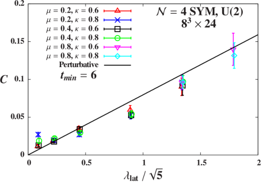
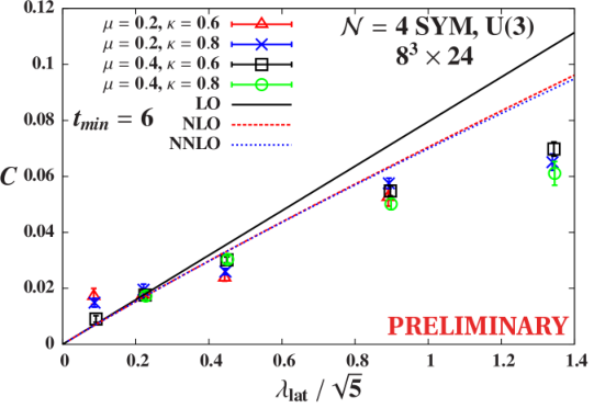
Fitting $V(r)$ to the Coulomb form $V(r)=A-C/r$, using all accessible $\sqrt{3/4}\leq r\leq 2.6$, produces the Coulomb coefficient results shown in Fig. 8. For each gauge group U(2) and U(3) we consider several values of $(\mu,\kappa)$, observing no significant dependence on these parameters. We plot the Coulomb coefficients as functions of the continuum ’t Hooft coupling $\lambda=\lambda_{\rm lat}/\sqrt{5}$, and compare our numerical results with perturbative predictions. For $N=2$ in the left panel of Fig. 8 we find values of $C$ in good agreement with leading-order (LO) perturbation theory,

$$C_{LO}=\frac{\lambda_{\rm lat}/\sqrt{5}}{4\pi}=\frac{\lambda}{4\pi}.$$

(24)

For $N=3$ in the right panel, however, our results begin deviating significantly from the LO line at stronger couplings. Although the next-to-leading-order and next-to-next-to-leading-order corrections from Refs. [22, 23, 24] move the perturbative prediction closer to our results, a clear difference remains. These NLO and NNLO contributions are

	$\displaystyle\frac{C_{NLO}}{C_{LO}}$	$\displaystyle=\frac{\lambda}{2\pi^{2}}\left(\log\left[\frac{\lambda}{2\pi}\right]+\gamma_{E}-1\right)$		(25)
	$\displaystyle\frac{C_{NNLO}}{C_{LO}}$	$\displaystyle=\frac{\lambda^{2}}{8\pi^{4}}\left\{\left(\log\left[\frac{\lambda}{2\pi}\right]+\gamma_{E}\right)^{2}+\left(1+\frac{\pi^{2}}{3}\right)\left(\log\left[\frac{\lambda}{2\pi}\right]+\gamma_{E}\right)-\frac{\pi^{2}}{12}-\frac{7}{2}+\frac{9}{4}\zeta(3)\right\}$

where $\gamma_{E}$ is Euler’s constant, $\zeta(3)\approx 1.202$ is Apéry’s constant, and we have set $C_{A}\alpha=2C_{F}\alpha=\frac{\lambda}{4\pi}$ for gauge group U($N$).

While it is tempting to interpret the right panel of Fig. 8 as a suggestion that we are seeing $C$ depart from perturbation theory to approach the famous large-$N$ prediction $C\propto\sqrt{\lambda}$ at strong coupling [25, 26], we suspect that both $N=3$ and $\lambda\leq 3/\sqrt{5}$ are still too small for this to happen. We can see that the NLO and (especially) NNLO corrections are still small compared to $C_{LO}$, suggesting that our results should remain within the perturbative regime. Although the contrast between $C$ for U(2) and U(3) in the two plots of Fig. 8 is striking, its cause is not yet clear. It will be very interesting to add U(4) results to this picture, to clarify any systematic trends. This work is underway, but is challenging due to the steeply increasing computation costs, which grow $\propto N^{5}$ [14].

Another interesting difference between the U(2) and U(3) static potentials is visible when we divide out the determinant of the Wilson loops from which $V(r)$ is extracted. As discussed in Section 4, this procedure should approximately project the observables to SU($N$), removing the U(1) sector that decouples in the continuum limit. We expect that the Coulomb coefficients $C_{D}$ resulting from determinant-divided Wilson loops will be reduced by a factor $(N^{2}-1)/N^{2}$ compared to the usual $C$ in Fig. 8. (This holds in perturbation theory through NLO, and the departure from this simple scaling at NNLO [24] appears negligible.)

In Fig. 9 we test our expectation by plotting the ratios $C_{D}/C$, again as functions of the continuum $\lambda=\lambda_{\rm lat}/\sqrt{5}$ for several values of $(\mu,\kappa)$. As before, there is no clear dependence on $(\mu,\kappa)$, and the ratios are also insensitive to the coupling. Our U(2) results are fairly noisy, but appear consistent with the expected ratio of $3/4$. In contrast, our results for $N=3$ are much more stable, which we emphasize by showing the same vertical range in both plots of Fig. 9. Numerically we find $C_{D}/C\approx 0.96$ with uncertainties small enough to clearly differ from the expected ratio of $8/9$. Again, ongoing investigations of U(4) will be important to clarify the interpretation of these initial U(3) results.

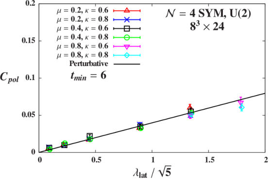
Finally, we can also consider the $\mathcal{N}=4$ static potential with the contribution of the scalar fields removed [22, 24]. We implement this by building Wilson loops from unitary matrices $u$ defined through the polar decomposition of each link variable, $\mathcal{U}=uH$ where $H$ is Hermitian and positive definite. Decoupling the scalar fields simplifies the perturbative predictions for the Coulomb coefficient in Refs. [22, 24], with Eqs. 24 and 25 becoming

$$\begin{split}C_{pol}&=\frac{\lambda}{8\pi}\left\{1-\frac{\lambda}{4\pi^{2}}+A\left(\frac{\lambda}{4\pi^{2}}\right)^{2}+B\left(\frac{\lambda}{4\pi^{2}}\right)^{3}\log\left[\frac{\lambda}{4\pi}\right]+\mathcal{O}\left(\lambda^{3}\right)\right\}\\ &\hskip 56.9055ptA=\frac{5}{4}+\frac{\pi^{2}}{4}-\frac{\pi^{4}}{64}\hskip 56.9055ptB=\frac{1}{12\pi}.\end{split}$$

(26)

At leading order the polar-projected $C_{pol}$ is just half the usual Coulomb coefficient, $C_{pol}/C=1/2$.

In Fig. 10 we plot $C_{pol}$ vs. $\lambda_{\rm lat}/\sqrt{5}$ for $N=2$ and 3, using the same axes and considering the same values of $(\mu,\kappa)$ as in Fig. 8. The U(2) results for $C_{pol}$ in the left panel of Fig. 10 are in good agreement with leading-order perturbation theory, and appear less noisy than the usual Coulomb coefficients in Fig. 8. The U(3) results in the right panel of Fig. 10 are significantly closer to leading-order perturbation theory than the corresponding $C$ in Fig. 8. At the same time, the higher-order perturbative corrections have barely visible effects in this range of $\lambda_{\rm lat}$. The $N=3$ $C_{pol}$ may still begin to drop below the perturbative predictions at the strongest coupling we have investigated so far, but this deviation is not significant and may be cured by extrapolating $(\mu,\kappa)\to(0,0)$.

Our investigations of lattice $\mathcal{N}=4$ SYM are making progress addressing a number of interesting questions, regarding both the validity of our lattice calculations as well as the resulting predictions that may be compared to continuum perturbation theory and gauge–gravity duality. In this proceedings, we presented several new developments that go beyond the results appearing in Refs. [12, 13]. These include an initial study of fine-tuning to recover the full symmetries of $\mathcal{N}=4$ SYM in the continuum limit, which makes use of the recent derivation that only a single parameter needs to be tuned so long as the moduli space is not lifted by nonperturbative effects. We also extended our measurements of the complex Pfaffian, considering more lattice volumes for larger $N=3$ and 4, which also indicate that the lattice theory does not suffer from a sign problem. These results provide additional evidence that our phase-quenched lattice calculations simulate $\mathcal{N}=4$ SYM to a good approximation, and can recover the appropriate theory in the continuum limit.

We then focused on the static potential, extending our previous study of gauge group U(2) with initial results for $N=3$. In both cases, we find Coulombic behavior at both weak and strong coupling, and compare the Coulomb coefficients to perturbation theory. Our initial U(3) results appear significantly less noisy than those for $N=2$, but fall away from perturbative predictions at the strongest couplings we have investigated. When we consider Wilson loops approximately projected to SU(3), we find Coulomb coefficients $C_{D}$ closer to the usual U(3) $C$ than we expected from naive $(N^{2}-1)/N^{2}$ scaling. It is not yet clear how we should interpret the current contrast between $N=2$ and 3. We are working on extending these investigations to $N=4$, which we hope will clarify any systematic trends.

Additional future work will include further studies of the Pfaffian phase, with the aim of improving our qualitative understanding of why we see no sign problem for lattice $\mathcal{N}=4$ SYM. Although it is extremely expensive to measure the Pfaffian on larger lattice volumes or for larger values of $N$, we may be able to gain insight by applying our new RG blocking scheme to obtain blocked systems with fewer degrees of freedom, which are more practical to analyze. MCRG analyses may also prove useful to predict the anomalous dimensions of single-trace operators like the Konishi, a particularly exciting goal. Such predictions would be complementary to those obtainable in perturbation theory [27] or via the conformal bootstrap program [28].

References

- [1] S. Catterall, D. B. Kaplan and M. Unsal, “Exact lattice supersymmetry”, Phys. Rept. 484 (2009) 71–130 [arXiv:0903.4881].
- [2] T. Ishii, G. Ishiki, S. Shimasaki and A. Tsuchiya, “ Super Yang–Mills from the Plane Wave Matrix Model”, Phys. Rev. D78 (2008) 106001 [arXiv:0807.2352].
- [3] G. Ishiki, S.-W. Kim, J. Nishimura and A. Tsuchiya, “Deconfinement phase transition in super Yang–Mills theory on from supersymmetric matrix quantum mechanics”, Phys. Rev. Lett. 102 (2009) 111601 [arXiv:0810.2884].
- [4] G. Ishiki, S.-W. Kim, J. Nishimura and A. Tsuchiya, “Testing a novel large-N reduction for super Yang–Mills theory on ”, JHEP 0909 (2009) 029 [arXiv:0907.1488].
- [5] M. Hanada, S. Matsuura and F. Sugino, “Two-dimensional lattice for four-dimensional supersymmetric Yang–Mills”, Prog. Theor. Phys. 126 (2011) 597–611 [arXiv:1004.5513].
- [6] M. Honda, G. Ishiki, J. Nishimura and A. Tsuchiya, “Testing the AdS/CFT correspondence by Monte Carlo calculation of BPS and non-BPS Wilson loops in 4d super-Yang–Mills theory”, PoS Lattice 2011 (2011) 244 [arXiv:1112.4274].
- [7] M. Honda, G. Ishiki, S.-W. Kim, J. Nishimura and A. Tsuchiya, “Direct test of the AdS/CFT correspondence by Monte Carlo studies of super Yang–Mills theory”, JHEP 1311 (2013) 200 [arXiv:1308.3525].
- [8] M. Hanada, Y. Hyakutake, G. Ishiki and J. Nishimura, “Holographic description of quantum black hole on a computer”, Science 344 (2014) 882–885 [arXiv:1311.5607].
- [9] S. Catterall, E. Dzienkowski, J. Giedt, A. Joseph and R. Wells, “Perturbative renormalization of lattice super Yang–Mills theory”, JHEP 1104 (2011) 074 [arXiv:1102.1725].
- [10] S. Catterall, P. H. Damgaard, T. Degrand, R. Galvez and D. Mehta, “Phase Structure of Lattice Super Yang–Mills”, JHEP 1211 (2012) 072 [arXiv:1209.5285].
- [11] S. Catterall, J. Giedt and A. Joseph, “Twisted supersymmetries in lattice super Yang–Mills theory”, JHEP 1310 (2013) 166 [arXiv:1306.3891].
- [12] S. Catterall, D. Schaich, P. H. Damgaard, T. DeGrand and J. Giedt, “ supersymmetry on a space-time lattice”, Phys. Rev. D90 (2014) 065013 [arXiv:1405.0644].
- [13] S. Catterall and J. Giedt, “Real space renormalization group for twisted lattice super Yang–Mills”, JHEP (in press, 2014) [arXiv:1408.7067].
- [14] D. Schaich and T. DeGrand, “Parallel software for lattice supersymmetric Yang–Mills theory”, arXiv:1410.6971.
- [15] N. Marcus, “The other topological twisting of Yang–Mills”, Nucl. Phys. B452 (1995) 331–345 [hep-th/9506002].
- [16] A. Kapustin and E. Witten, “Electric-Magnetic Duality And The Geometric Langlands Program”, Commun. Num. Theor. Phys. 1 (2007) 1–236 [hep-th/0604151].
- [17] M. Ünsal, “Twisted supersymmetric gauge theories and orbifold lattices”, JHEP 0610 (2006) 089 [hep-th/0603046].
- [18] F. Palumbo, “Gauge Invariance on the Lattice With Noncompact Gauge Fields”, Phys. Lett. B244 (1990) 55–57.
- [19] C. M. Becchi and F. Palumbo, “Noncompact gauge theories on a lattice: Perturbative study of the scaling properties”, Nucl. Phys. B388 (1992) 595–608.
- [20] F. Palumbo and R. Scimia, “Noncompact gauge fields on a lattice: SU() theories”, Phys. Rev. D65 (2002) 074509 [hep-lat/0105029].
- [21] T. A. DeGrand and D. Toussaint, “Topological Excitations and Monte Carlo Simulation of Abelian Gauge Theory”, Phys. Rev. D22 (1980) 2478.
- [22] A. Pineda, “Static potential in supersymmetric Yang-Mills at weak coupling”, Phys. Rev. D77 (2008) 021701 [arXiv:0709.2876].
- [23] M. Stahlhofen, “NLL resummation for the static potential in SYM theory”, JHEP 1211 (2012) 155 [arXiv:1209.2122].
- [24] M. Prausa and M. Steinhauser, “Two-loop static potential in supersymmetric Yang-Mills theory”, Phys. Rev. D88 (2013) 025029 [arXiv:1306.5566].
- [25] S.-J. Rey and J.-T. Yee, “Macroscopic strings as heavy quarks in large N gauge theory and anti-de Sitter supergravity”, Eur. Phys. J. C22 (2001) 379–394 [hep-th/9803001].
- [26] J. M. Maldacena, “Wilson loops in large N field theories”, Phys. Rev. Lett. 80 (1998) 4859–4862 [hep-th/9803002].
- [27] C. Beem, L. Rastelli, A. Sen and B. C. van Rees, “Resummation and S-duality in SYM”, JHEP 1404 (2014) 122 [arXiv:1306.3228].
- [28] C. Beem, L. Rastelli and B. C. van Rees, “ Superconformal Bootstrap”, Phys. Rev. Lett. 111 (2013) 071601 [arXiv:1304.1803].