跳到论文正文
W Papers独立论文阅读器 arXiv:1411.0073 论文正文 计算阅读时间 · 0%
引用这篇论文根据当前论文元数据生成,正式投稿前建议核对。


License: arXiv.org perpetual non-exclusive license
arXiv:1411.0073v1 [stat.ML] 01 Nov 2014

Learning Mixed Multinomial Logit Model from Ordinal Data

Sewoong Oh Affiliation: Dept. of Industrial and Enterprise Systems Engr. Affiliation: University of Illinois at Urbana-Champaign Affiliation: Urbana, IL 61801 Email: swoh@illinois.edu    Devavrat Shah Affiliation: Department of Electrical Engineering Affiliation: Massachussetts Institute of Technology Affiliation: Cambridge, MA 02139 Email: devavrat@mit.edu
Abstract

Motivated by generating personalized recommendations using ordinal (or preference) data, we study the question of learning a mixture of MultiNomial Logit (MNL) model, a parameterized class of distributions over permutations, from partial ordinal or preference data (e.g. pair-wise comparisons). Despite its long standing importance across disciplines including social choice, operations research and revenue management, little is known about this question. In case of single MNL models (no mixture), computationally and statistically tractable learning from pair-wise comparisons is feasible. However, even learning mixture with two MNL components is infeasible in general.

Given this state of affairs, we seek conditions under which it is feasible to learn the mixture model in both computationally and statistically efficient manner. We present a sufficient condition as well as an efficient algorithm for learning mixed MNL models from partial preferences/comparisons data. In particular, a mixture of rr MNL components over nn objects can be learnt using samples whose size scales polynomially in nn and rr (concretely, r3.5​n3​(log⁡n)4r^{3.5}n^{3}(\log n)^{4}, with r≪n2/7r\ll n^{2/7} when the model parameters are sufficiently incoherent). The algorithm has two phases: first, learn the pair-wise marginals for each component using tensor decomposition; second, learn the model parameters for each component using RankCentrality introduced by Negahban et al. In the process of proving these results, we obtain a generalization of existing analysis for tensor decomposition to a more realistic regime where only partial information about each sample is available.


1 Introduction

Background. Popular recommendation systems such as collaborative filtering are based on a partially observed ratings matrix. The underlying hypothesis is that the true/latent score matrix is low-rank and we observe its partial, noisy version. Therefore, matrix completion algorithms are used for learning, cf. [8, 14, 15, 20]. In reality, however, observed preference data is not just scores. For example, clicking one of the many choices while browsing provides partial order between clicked choice versus other choices. Further, scores do convey ordinal information as well, e.g. score of 4 for paper A and score of 7 for paper B by a reviewer suggests ordering B >> A. Similar motivations led Samuelson to propose the Axiom of revealed preference [21] as the model for rational behavior. In a nutshell, it states that consumers have latent order of all objects, and the revealed preferences through actions/choices are consistent with this order. If indeed all consumers had identical ordering, then learning preference from partial preferences is effectively the question of sorting.

In practice, individuals have different orderings of interest, and further, each individual is likely to make noisy choices. This naturally suggests the following model – each individual has a latent distribution over orderings of objects of interest, and the revealed partial preferences are consistent with it, i.e. samples from the distribution. Subsequently, the preference of the population as a whole can be associated with a distribution over permutations. Recall that the low-rank structure for score matrices, as a model, tries to capture the fact that there are only a few different types of choice profile. In the context of modeling consumer choices as distribution over permutation, MultiNomial Logit (MNL) model with a small number of mixture components provides such a model.

Mixed MNL. Given nn objects or choices of interest, an MNL model is described as a parametric distribution over permutations of nn with parameters 𝐰=[wi]∈ℝn{\bf w}=[w_{i}]\in{\mathbb{R}}^{n}: each object i,1≤i≤ni,~1\leq i\leq n, has a parameter wi>0w_{i}>0 associated with it. Then the permutations are generated randomly as follows: choose one of the nn objects to be ranked 11 at random, where object ii is chosen to be ranked 11 with probability wi/(∑j=1nwj)w_{i}/(\sum_{j=1}^{n}w_{j}). Let i1i_{1} be object chosen for the first position. Now to select second ranked object, choose from remaining with probability proportional to their weight. We repeat until all objects for all ranked positions are chosen. It can be easily seen that, as per this model, an item ii is ranked higher than jj with probability wi/(wi+wj)w_{i}/(w_{i}+w_{j}).

In the mixed MNL model with r≥2r\geq 2 mixture components, each component corresponds to a different MNL model: let 𝐰(1),…,𝐰(r){\bf w}^{(1)},\dots,{\bf w}^{(r)} be the corresponding parameters of the rr components. Let 𝐪=[qa]∈[0,1]r{\bf q}=[q_{a}]\in[0,1]^{r} denote the mixture distribution, i.e. ∑aqa=1\sum_{a}q_{a}=1. To generate a permutation at random, first choose a component a∈{1,…,r}a\in\{1,\dots,r\} with probability qaq_{a}, and then draw random permutation as per MNL with parameters 𝐰(a){\bf w}^{(a)}.

Brief history. The MNL model is an instance of a class of models introduced by Thurstone [23]. The description of the MNL provided here was formally established by McFadden [17]. The same model (in form of pair-wise marginals) was introduced by Zermelo [25] as well as Bradley and Terry [7] independently. In [16], Luce established that MNL is the only distribution over permutation that satisfies the axiom of Independence from Irrelevant Alternatives.

On learning distributions over permutations, the question of learning single MNL model and more generally instances of Thurstone’s model have been of interest for quite a while now. The maximum likelihood estimator, which is logistic regression for MNL, has been known to be consistent in large sample limit, cf. [13]. Recently, RankCentrality [19] was established to be statistical efficient. For learning sparse mixture model, i.e. distribution over permutations with each mixture being delta distribution, [11] provided sufficient conditions under which mixtures can be learnt exactly using pair-wise marginals – effectively, as long as the number of components scaled as o⁡(log⁡n)o(\log n) where components satisfied appropriate incoherence condition, a simple iterative algorithm could recover the mixture. However, it is not robust with respect to noise in data or finite sample error in marginal estimation. Other approaches have been proposed to recover model using convex optimization based techniques, cf. [10, 18]. MNL model is a special case of a larger family of discrete choice models known as the Random Utility Model (RUM), and an efficient algorithm to learn RUM is introduced in [22]. Efficient algorithms for learning RUMs from partial rankings has been introduced in [3, 4]. We note that the above list of references is very limited, including only closely related literature. Given the nature of the topic, there are a lot of exciting lines of research done over the past century and we shall not be able to provide comprehensive coverage due to a space limitation.

Problem. Given observations from the mixed MNL, we wish to learn the model parameters, the mixing distribution 𝐪{\bf q}, and parameters of each component 𝐰(1),…,𝐰(r){\bf w}^{(1)},\dots,{\bf w}^{(r)}. The observations are in form of pair-wise comparisons. Formally, to generate an observation, first one of the rr mixture components is chosen; and then for ℓ\ell of all possible (n2){n\choose 2} pairs, comparison outcome is observed as per this MNL component11 1 We shall assume that, outcomes of these ℓ\ell pairs are independent of each other, but coming from the same MNL mixture component. This is effectively true even they were generated by first sampling a permutation from the chosen MNL mixture component, and then observing implication of this permutation for the specific ℓ\ell pairs, as long as they are distinct due to the Irrelevance of Independent Alternative hypothesis of Luce that is satisfied by MNL.. These ℓ\ell pairs are chosen, uniformly at random, from a pre-determined N≤(n2)N\leq{n\choose 2} pairs: {(ik,jk),1≤k≤N}\{(i_{k},j_{k}),1\leq k\leq N\}. We shall assume that the selection of NN is such that the undirected graph G=([n],E)G=([n],E), where E={(ik,jk):1≤k≤N}E=\{(i_{k},j_{k}):1\leq k\leq N\}, is connected.

We ask following questions of interest: Is it always feasible to learn mixed MNL? If not, under what conditions and how many samples are needed? How computationally expensive are the algorithms?

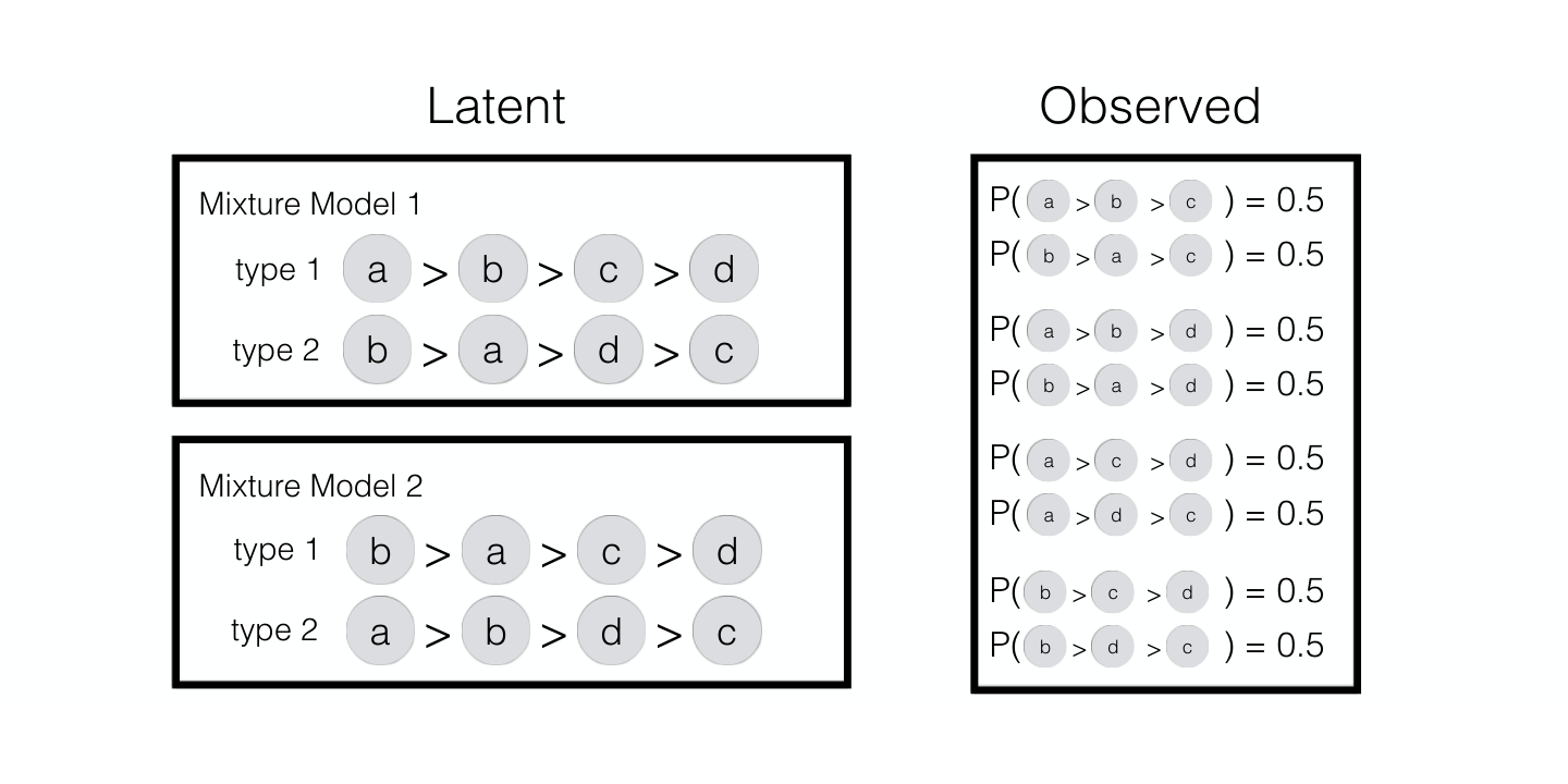
We briefly recall a recent result [1] that suggests that it is impossible to learn mixed MNL models in general. One such example is described in Figure 1. It depicts an example with n=4n=4 and r=2r=2 and a uniform mixture distribution. For the first case, in mixture component 11, with probability 11 the ordering is a>b>c>da>b>c>d (we denote n=4n=4 objects by a,b,ca,b,c and dd); and in mixture component 22, with probability 11 the ordering is b>a>d>cb>a>d>c. Similarly for the second case, the two mixtures are made up of permutations b>a>c>db>a>c>d and a>b>d>ca>b>d>c. It is easy to see the distribution over any 33-wise comparisons generated from these two mixture models is identical. Therefore, it is impossible to differentiate these two using 33-wise or pair-wise comparisons. In general, [1] established that there exist mixture distributions with r≤n/2r\leq n/2 over nn objects that are impossible to distinguish using log⁡n\log n-wise comparison data. That is, learning mixed MNL is not always possible.
Refer to caption
Figure 1: Two mixture models that cannot be differentiated even with 33-wise preference data.

Contributions. The main contribution of this work is identification of sufficient conditions under which mixed MNL model can be learnt efficiently, both statistically and computationally. Concretely, we propose a two-phase learning algorithm: in the first phase, using a tensor decomposition method for learning mixture of discrete product distribution, we identify pair-wise marginals associated with each of the mixture; in the second phase, we use these pair-wise marginals associated with each mixture to learn the parameters associated with each of the MNL mixture component.

The algorithm in the first phase builds upon the recent work by Jain and Oh [12]. In particular, Theorem 3 generalizes their work for the setting where for each sample, we have limited information - as per [12], we would require that each individual gives the entire permutation; instead, we have extended the result to be able to cope with the current setting when we only have information about ℓ\ell, potentially finite, pair-wise comparisons. The algorithm in the second phase utilizes RankCentrality [19]. Its analysis in Theorem 4 works for setting where observations are no longer independent, as required in [19].

We find that as long as certain rank and incoherence conditions are satisfied by the parameters of each of the mixture, the above described two phase algorithm is able to learn mixture distribution 𝐪{\bf q} and parameters associated with each mixture, 𝐰(1),…,𝐰(r){\bf w}^{(1)},\dots,{\bf w}^{(r)} faithfully using samples that scale polynomially in nn and rr – concretely, the number of samples required scale as r3.5​n3​(log⁡n)4r^{3.5}n^{3}(\log n)^{4} with constants dependent on the incoherence between mixture components, and as long as r≪n2/7r\ll n^{2/7} as well as GG, the graph of potential comparisons, is a spectral expander with the total number of edges scaling as N=O⁡(n​log⁡n)N=O(n\log n). For the precise statement, we refer to Theorem 1.

The algorithms proposed are iterative, and primarily based on spectral properties of underlying tensors/matrices with provable, fast convergence guarantees. That is, algorithms are not only polynomial time, they are practical enough to be scalable for high dimensional data sets.

Notations. We use [N]={1,…,N}[N]=\{1,\ldots,N\} for the first NN positive integers. We use ⊗\otimes to denote the outer product such that (x⊗y⊗z)i​j​k=xi​yj​zk(x\otimes y\otimes z)_{ijk}=x_{i}y_{j}z_{k}. Given a third order tensor T∈ℝn1×n2×n3T\in{\mathbb{R}}^{n_{1}\times n_{2}\times n_{3}} and a matrix U∈ℝn1×r1,V∈ℝn2×r2,W∈ℝn3×r3U\in{\mathbb{R}}^{n_{1}\times r_{1}},V\in{\mathbb{R}}^{n_{2}\times r_{2}},W\in{\mathbb{R}}^{n_{3}\times r_{3}}, we define a linear mapping T⁡[U,V,W]∈ℝr1×r2×r3T[U,V,W]\in{\mathbb{R}}^{r_{1}\times r_{2}\times r_{3}} as T​[U,V,W]a​b​c=∑i,j,kTi​j​k​Ui​a​Vj​b​Wk​cT[U,V,W]_{abc}=\sum_{i,j,k}T_{ijk}U_{ia}V_{jb}W_{kc}. We let ‖x‖=∑ixi2\|x\|=\sqrt{\sum_{i}x_{i}^{2}} be the Euclidean norm of a vector, ‖M‖2=max‖x‖≤1,‖y‖≤1⁡xT​M​y\|M\|_{2}=\max_{\|x\|\leq 1,\|y\|\leq 1}x^{T}My be the operator norm of a matrix, and ‖M‖F=∑i,jMi​j2\|M\|_{F}=\sqrt{\sum_{i,j}M_{ij}^{2}} be the Frobenius norm. We say an event happens with high probability (w.h.p) if the probability is lower bounded by 1−f⁡(n)1-f(n) such that f⁡(n)=o⁡(1)f(n)=o(1) as nn scales to ∞\infty.

2 Main result

In this section, we describe the main result: sufficient conditions under which mixed MNL models can be learnt using tractable algorithms. We provide a useful illustration of the result as well as discuss its implications.

Definitions. Let 𝒮{\cal S} denote the collection of observations, each of which is denoted as NN dimensional, {−1,0,+1}\{-1,0,+1\} valued vector. Recall that each observation is obtained by first selecting one of the rr mixture MNL component, and then viewing outcomes, as per the chosen MNL mixture component, of ℓ\ell randomly chosen pair-wise comparisons from the NN pre-determined comparisons {(ik,jk):1≤ik≠jk≤n,1≤k≤N}\{(i_{k},j_{k}):1\leq i_{k}\neq j_{k}\leq n,1\leq k\leq N\}. Let xt∈{−1,0,+1}Nx_{t}\in\{-1,0,+1\}^{N} denote the ttth observation with xt,k=0x_{t,k}=0 if the kkth pair (ik,jk)(i_{k},j_{k}) is not chosen amongst the ℓ\ell randomly chosen pairs, and xt,k=+1x_{t,k}=+1 (respectively −1-1) if ik<jki_{k}<j_{k} (respectively ik>jki_{k}>j_{k}) as per the chosen MNL mixture component. By definition, it is easy to see that for any t∈𝒮t\in{\cal S} and 1≤k≤N1\leq k\leq N,

𝔼⁡[xt,k]\displaystyle\mathbb{E}[x_{t,k}] =ℓN​[∑a=1rqa​Pk​a],where​Pk​a=wjk(a)−wik(a)wjk(a)+wik(a).\displaystyle=\frac{\ell}{N}\Big[\sum_{a=1}^{r}q_{a}P_{ka}\Big],~\mbox{where}~P_{ka}=\frac{w_{j_{k}}^{(a)}-w_{i_{k}}^{(a)}}{w_{j_{k}}^{(a)}+w_{i_{k}}^{(a)}}. (1)

We shall denote Pa=[Pk​a]∈[−1,1]NP_{a}=[P_{ka}]\in[-1,1]^{N} for 1≤a≤r1\leq a\leq r. Therefore, in a vector form

𝔼⁡[xt]\displaystyle\mathbb{E}[x_{t}] =ℓN​P​𝐪,where​P=[P1​…​Pr]∈[−1,1]N×r.\displaystyle=\frac{\ell}{N}P{\bf q},~\mbox{where}~~P=[P_{1}\dots P_{r}]\in[-1,1]^{N\times r}\;. (2)

That is, PP is a matrix with rr columns, each representing one of the rr mixture components and 𝐪{\bf q} is the mixture probability. By independence, for any t∈𝒮t\in{\cal S}, and any two different pairs 1≤k≠m≤N1\leq k\neq m\leq N,

𝔼⁡[xt,k​xt,m]\displaystyle\mathbb{E}[x_{t,k}x_{t,m}] =ℓ2N2​[∑a=1rqa​Pk​a​Pm​a].\displaystyle=\frac{\ell^{2}}{N^{2}}\Big[\sum_{a=1}^{r}q_{a}P_{ka}P_{ma}\Big]. (3)

Therefore, the N×NN\times N matrix 𝔼⁡[xt​xtT]\mathbb{E}[x_{t}x_{t}^{T}] or equivalently tensor 𝔼⁡[xt⊗xt]\mathbb{E}[x_{t}\otimes x_{t}] is proportional to M2M_{2} except in diagonal entries, where

M2\displaystyle M_{2} =P​Q​PT≡∑a=1rqa​(Pa⊗Pa),\displaystyle=PQP^{T}\equiv\sum_{a=1}^{r}q_{a}(P_{a}\otimes P_{a})\;, (4)

Q=diag⁡(𝐪)Q={\rm diag}({\bf q}) being diagonal matrix with its entries being mixture probabilities, 𝐪{\bf q}. In a similar manner, the tensor 𝔼⁡[xt⊗xt⊗xt]\mathbb{E}[x_{t}\otimes x_{t}\otimes x_{t}] is proportional to M3M_{3} (except in O⁡(N2)O(N^{2}) entries), where

M3\displaystyle M_{3} =∑a=1rqa​(Pa⊗Pa⊗Pa).\displaystyle=\sum_{a=1}^{r}q_{a}(P_{a}\otimes P_{a}\otimes P_{a}). (5)

Indeed, empirical estimates M^2\hat{M}_{2} and M^3\hat{M}_{3}, defined as

M^2\displaystyle\hat{M}_{2} =1|𝒮|​[∑t∈𝒮xt⊗xt],and​M^3=1|𝒮|​[∑t∈𝒮xt⊗xt⊗xt],\displaystyle=\frac{1}{|{\cal S}|}\Big[\sum_{t\in{\cal S}}x_{t}\otimes x_{t}\Big],~\mbox{and}~\hat{M}_{3}=\frac{1}{|{\cal S}|}\Big[\sum_{t\in{\cal S}}x_{t}\otimes x_{t}\otimes x_{t}\Big], (6)

provide good proxy for M2M_{2} and M3M_{3} for large enough number of samples; and shall be utilized crucially for learning model parameters from observations.

Sufficient conditions for learning. With the above discussion, we state sufficient conditions for learning the mixed MNL in terms of properties of M2M_{2}:

  • C1.

    M2M_{2} has rank rr; let σ1​(M2)\sigma_{1}(M_{2}), σr​(M2)>0\sigma_{r}(M_{2})>0 be the largest and smallest singular values of M2M_{2}.

  • C2.

    For a large enough universal constant C′>0C^{\prime}>0,

    N\displaystyle N ≥C′​r3.5​μ6​(M2)​(σ1​(M2)σr​(M2))4.5.\displaystyle\geq C^{\prime}{r^{3.5}\,\mu^{6}(M_{2})}\,\Big(\frac{\sigma_{1}(M_{2})}{\sigma_{r}(M_{2})}\Big)^{4.5}. (7)

    In the above, μ⁡(M2)\mu(M_{2}) represents incoherence of a symmetric matrix M2M_{2}. We recall that for a symmetric matrix M∈ℝN×NM\in{\mathbb{R}}^{N\times N} of rank rr with singular value decomposition M=U​S​UTM=USU^{T}, the incoherence is defined as

    μ⁡(M)\displaystyle\mu(M) =Nr​(maxi∈[N]⁡‖Ui‖).\displaystyle=\sqrt{\frac{N}{r}}\Big(\max_{i\in[N]}\|U_{i}\|\Big). (8)
  • C3.

    The undirected graph G=([n],E)G=([n],E) with E={(ik,jk):1≤k≤N}E=\{(i_{k},j_{k}):1\leq k\leq N\} is connected. Let A∈{0,1}n×nA\in\{0,1\}^{n\times n} be adjacency matrix with Ai​j=1A_{ij}=1 if (i,j)∈E(i,j)\in E and 00 otherwise; let D=diag⁡(di)D={\rm diag}(d_{i}) with did_{i} being degree of vertex i∈[n]i\in[n] and let LG=D−1​AL_{G}=D^{-1}A be normalized Laplacian of GG. Let dmax=maxi⁡did_{\rm max}=\max_{i}d_{i} and dmin=mini⁡did_{\rm min}=\min_{i}d_{i}. Let the nn eigenvalues of stochastic matrix LGL_{G} be 1=λ1​(LG)≥…​λn​(LG)≥−11=\lambda_{1}(L_{G})\geq\dots\lambda_{n}(L_{G})\geq-1. Define spectral gap of GG:

    ξ⁡(G)\displaystyle\xi(G) =1−max⁡{λ2​(L),−λn​(L)}.\displaystyle=1-\max\{\lambda_{2}(L),-\lambda_{n}(L)\}. (9)

Note that we choose a graph G=([n],E)G=([n],E) to collect pairwise data on, and we want to use a graph that is connected, has a large spectral gap, and has a small number of edges. In condition (C3), we need connectivity since we cannot estimate the relative strength between disconnected components (e.g. see [13]). Further, it is easy to generate a graph with spectral gap ξ⁡(G)\xi(G) bounded below by a universal constant (e.g. 1/1001/100) and the number of edges N=O⁡(n​log⁡n)N=O(n\log n), for example using the configuration model for Erdös-Renyi graphs. In condition (C2), we require the matrix M2M_{2} to be sufficiently incoherent with bounded σ1​(M2)/σr​(M2)\sigma_{1}(M_{2})/\sigma_{r}(M_{2}). For example, if qmax/qmin=O⁡(1)q_{\rm max}/q_{\rm min}=O(1) and the profile of each type in the mixture distribution is sufficiently different, i.e. ⟨Pa,Pb⟩/(‖Pa‖​‖Pb‖)<1/(2​r)\langle P_{a},P_{b}\rangle/(\|P_{a}\|\|P_{b}\|)<1/(2r), then we have μ⁡(M2)=O⁡(1)\mu(M_{2})=O(1) and σ1​(M2)/σr​(M2)=O⁡(1)\sigma_{1}(M_{2})/\sigma_{r}(M_{2})=O(1). We define b=maxa=1r​maxi,j∈[n]​wi(a)/wj(a)b=\max_{a=1}^{r}\max_{i,j\in[n]}{w^{(a)}_{i}}/{w^{(a)}_{j}}, qmax=maxa⁡qaq_{\rm max}=\max_{a}q_{a}, and qmin=mina⁡qaq_{\rm min}=\min_{a}q_{a}. The following theorem provides a bound on the error and we refer to the appendix for a proof.

Theorem 1.

Consider a mixed MNL model satisfying conditions (C1)-(C3). Then for any δ∈(0,1)\delta\in(0,1), there exists positive numerical constants C,C′C,C^{\prime} such that for any positive ε\varepsilon satisfying

0<ε<(qmin​ξ2​(G)​dmin216​qmax​r​σ1​(M2)​b5​dmax2)0.5,\displaystyle 0<\varepsilon<~\Big(\frac{q_{\rm min}\xi^{2}(G)d_{\rm min}^{2}}{16q_{\rm max}\,r\,\sigma_{1}(M_{2})b^{5}d_{\rm max}^{2}}\Big)^{0.5}, (10)

Algorithm 1 produces estimates 𝐪^=[q^a]\hat{{\bf q}}=[\hat{q}_{a}] and 𝐰^=[𝐰^(a)]\hat{{\bf w}}=[\hat{{\bf w}}^{(a)}] so that with probability at least 1−δ1-\delta,

|q^a−qa|\displaystyle\big|\;\hat{q}_{a}-q_{a}\;\big| ≤ε, and\displaystyle\leq\varepsilon,\text{ and }
‖𝐰^(a)−𝐰(a)‖‖𝐰(a)‖\displaystyle\frac{\|\hat{{\bf w}}^{(a)}-{\bf w}^{(a)}\|}{\|{\bf w}^{(a)}\|} ≤C​(r​qmax​σ1​(M2)​b5​dmax2qmin​ξ2​(G)​dmin2)0.5​ε,\displaystyle\leq C\Big(\frac{r\,q_{\rm max}\,\sigma_{1}(M_{2})b^{5}d_{\rm max}^{2}}{q_{\rm min}\xi^{2}(G)d_{\rm min}^{2}}\Big)^{0.5}~\varepsilon, (11)

for all a∈[r]a\in[r], as long as

|𝒮|\displaystyle|{\cal S}| ≥C′​r​N4​log⁡(N/δ)qmin​σ1​(M2)2​ε2​(1ℓ2+σ1​(M2)ℓ​N+r4​σ1​(M2)4σr​(M2)5).\displaystyle\geq C^{\prime}\frac{rN^{4}\log(N/\delta)}{q_{\rm min}\sigma_{1}(M_{2})^{2}\varepsilon^{2}}\Big(\frac{1}{\ell^{2}}+\frac{\sigma_{1}(M_{2})}{\ell N}+\frac{r^{4}\sigma_{1}(M_{2})^{4}}{\sigma_{r}(M_{2})^{5}}\Big)\;. (12)

An illustration of Theorem 1. To understand the applicability of Theorem 1, consider a concrete example with r=2r=2; let the corresponding weights 𝐰(1){\bf w}^{(1)} and 𝐰(2){\bf w}^{(2)} be generated by choosing each weight uniformly from [1,2][1,2]. In particular, the rank order for each component is a uniformly random permutation. Let the mixture distribution be uniform as well, i.e. 𝐪=[0.5​0.5]{\bf q}=[0.5~0.5]. Finally, let the graph G=([n],E)G=([n],E) be chosen as per the Erdös-Rényi model with each edge chosen to be part of the graph with probability d¯/n\bar{d}/n, where d¯>log⁡n\bar{d}>\log n. For this example, it can be checked that Theorem 1 guarantees that for ε≤C/n​d¯\varepsilon\leq C/\sqrt{n\bar{d}}, |𝒮|≥C′​n2​d¯2​log⁡(n​d¯/δ)/(ℓ​ε2)|{\cal S}|\geq C^{\prime}n^{2}\bar{d}^{2}\log(n\bar{d}/\delta)/(\ell\varepsilon^{2}), and n​d¯≥C′n\bar{d}\geq C^{\prime}, we have for all a∈{1,2}a\in\{1,2\}, |q^a−qa|≤ε|\hat{q}_{a}-q_{a}|\leq\varepsilon and ‖𝐰^(a)−𝐰(a)‖/‖𝐰(a)‖≤C′′​n​d¯​ε\|\hat{{\bf w}}^{(a)}-{\bf w}^{(a)}\|/\|{\bf w}^{(a)}\|\leq C^{\prime\prime}\sqrt{n\bar{d}}\,\varepsilon. That is, for ℓ=Θ⁡(1)\ell=\Theta(1) and choosing ε=ε′/(n​d¯)\varepsilon=\varepsilon^{\prime}/(\sqrt{n\bar{d}}), we need sample size of |𝒮|=O⁡(n3​d¯3​log⁡n)|{\cal S}|=O(n^{3}\bar{d}^{3}\log n) to guarantee error in both 𝐪^\hat{{\bf q}} and 𝐰^\hat{{\bf w}} smaller than ε′\varepsilon^{\prime}. Instead, if we choose ℓ=Θ⁡(n​d¯)\ell=\Theta(n\bar{d}), we only need |𝒮|=O⁡((n​d¯)2​log⁡n)|{\cal S}|=O((n\bar{d})^{2}\log n). Limited samples per observation leads to penalty of factor of (n​d¯/ℓ)(n\bar{d}/\ell) in sample complexity. To provide bounds on the problem parameters for this example, we use standard concentration arguments. It is well known for Erdös-Rényi random graphs (see [6]) that, with high probability, the number of edges concentrates in [(1/2)​d¯​n,(3/2)​d¯​n][(1/2)\bar{d}\,n,(3/2)\bar{d}\,n] implying N=Θ⁡(d¯​n)N=\Theta(\bar{d}n), and the degrees also concentrate in [(1/2)​d¯,(3/2)​d¯][(1/2)\bar{d},(3/2)\bar{d}], implying dmax=dmin=Θ⁡(d¯)d_{\rm max}=d_{\rm min}=\Theta(\bar{d}). Also using standard concentration arguments for spectrum of random matrices, it follows that the spectral gap of GG is bounded by ξ≥1−(C/d¯)=Θ⁡(1)\xi\geq 1-(C/\sqrt{\bar{d}})=\Theta(1) w.h.p. Since we assume the weights to be in [1,2][1,2], the dynamic range is bounded by b≤2b\leq 2. The following Proposition shows that σ1​(M2)=Θ⁡(N)=Θ⁡(d¯​n)\sigma_{1}(M_{2})=\Theta(N)=\Theta(\bar{d}n), σ2​(M2)=Θ⁡(d¯​n)\sigma_{2}(M_{2})=\Theta(\bar{d}n), and μ⁡(M2)=Θ⁡(1)\mu(M_{2})=\Theta(1).

Proposition 2.1.

For the above example, when d¯≥log⁡n\bar{d}\geq\log n, σ1​(M2)≤0.02​N\sigma_{1}(M_{2})\leq 0.02N, σ2​(M2)≥0.017​N\sigma_{2}(M_{2})\geq 0.017N, and μ⁡(M2)≤15\mu(M_{2})\leq 15 with high probability.

Supposen now for general rr, we are interested in well-behaved scenario where qmax=Θ⁡(1/r)q_{\rm max}=\Theta(1/r) and qmin=Θ⁡(1/r)q_{\rm min}=\Theta(1/r). To achieve arbitrary small error rate for ‖𝐰^(a)−𝐰(a)‖/‖𝐰(a)‖\|\hat{{\bf w}}^{(a)}-{\bf w}^{(a)}\|/\|{\bf w}^{(a)}\|, we need ϵ=O⁡(1/r​N)\epsilon=O(1/\sqrt{r\,N}), which is achieved by sample size |𝒮|=O⁡(r3.5​n3​(log⁡n)4)|{\cal S}|=O(r^{3.5}n^{3}(\log n)^{4}) with d¯=log⁡n\bar{d}=\log n.

3 Algorithm

We describe the algorithm achieving the bound in Theorem 1. Our approach is two-phased. First, learn the moments for mixtures using a tensor decomposition, cf. Algorithm 2: for each type a∈[r]a\in[r], produce estimate q^a∈ℝ\hat{q}_{a}\in{\mathbb{R}} of the mixture weight qaq_{a} and estimate P^a=[P^1​a​…​P^N​a]T∈ℝN\hat{P}_{a}=[\hat{P}_{1a}\,\ldots\,\hat{P}_{Na}]^{T}\in{\mathbb{R}}^{N} of the expected outcome Pa=[P1​a​…​PN​a]TP_{a}=[P_{1a}\,\ldots\,P_{Na}]^{T} defined as in (1). Secondly, for each aa, using the estimate P^a\hat{P}_{a}, apply RankCentrality, cf. Section 3.2, to estimate 𝐰^(a)\hat{{\bf w}}^{(a)} for the MNL weights 𝐰(a){\bf w}^{(a)}.

Algorithm 1
1:  Input: Samples {xt}t∈𝒮\{x_{t}\}_{t\in{\cal S}}, number of types rr, number of iterations T1,T2T_{1},T_{2}, graph G⁡([n],E)G([n],E)
2:  {(q^a,P^a)}a∈[r]←SpectralDist​({xt}t∈𝒮,r,T1)\{(\hat{q}_{a},\hat{P}_{a})\}_{a\in[r]}\leftarrow\text{\sc SpectralDist}\left(\{x_{t}\}_{t\in{\cal S}},r,T_{1}\right) (see Algorithm 2)
3:  for a=1,…,ra=1,\ldots,r do
4:   set P~a←𝒫[−1,1]​(P^a){\tilde{P}}_{a}\leftarrow{\cal P}_{[-1,1]}(\hat{P}_{a}) where 𝒫[−1,1]​(⋅){\cal P}_{[-1,1]}(\cdot) is the projection onto [−1,1]N[-1,1]^{N}
5:   w^(a)←RankCentrality​(G,P~a,T2){\hat{w}}^{(a)}\leftarrow\text{\sc RankCentrality}\left(G,{\tilde{P}}_{a},T_{2}\right) (see Section 3.2)
6:  end for
7:  Output: {(q^(a),𝐰^(a))}a∈[r]\{(\hat{q}^{(a)},\hat{{\bf w}}^{(a)})\}_{a\in[r]}

To achieve Theorem 1, T1=Θ⁡(log⁡(N​|𝒮|))T_{1}=\Theta\big(\log(N\,|{\cal S}|)\big) and T2=Θ⁡(b2​dmax​(log⁡n+log⁡(1/ε))/(ξ​dmin))T_{2}=\Theta\big(\,b^{2}d_{\rm max}(\log n+\log(1/\varepsilon))/(\xi d_{\rm min})\,\big) is sufficient. Next, we describe the two phases of algorithms and associated technical results.

3.1 Phase 1: Spectral decomposition.

To estimate PP and 𝐪{\bf q} from the samples, we shall use tensor decomposition of M^2\hat{M}_{2} and M3^\hat{M_{3}}, the empirical estimation of M2M_{2} and M3M_{3} respectively, recall (4)-(6). Let M2=UM2​ΣM2​UM2TM_{2}=U_{M_{2}}\Sigma_{M_{2}}U_{M_{2}}^{T} be the eigenvalue decomposition and let

H\displaystyle H =\displaystyle= M3[UM2ΣM2−1/2,UM2ΣM2−1/2,UM2ΣM2−1/2].\displaystyle M_{3}[U_{M_{2}}\Sigma_{M_{2}}^{-1/2},U_{M_{2}}\Sigma_{M_{2}}^{-1/2},U_{M_{2}}\Sigma_{M_{2}}^{-1/2}]\;.

The next theorem shows that M2M_{2} and M3M_{3} are sufficient to learn PP and 𝐪{\bf q} exactly, when M2M_{2} has rank rr (throughout, we assume that r≪n≤Nr\ll n\leq N).

Theorem 2 (Theorem 3.1 [12]).

Let M2∈ℝN×NM_{2}\in{\mathbb{R}}^{N\times N} have rank rr. Then there exists an orthogonal matrix VH=[v1H​v2H​…​vrH]∈ℝr×rV^{H}=[v^{H}_{1}\;v^{H}_{2}\;\ldots\;v^{H}_{r}]\in{\mathbb{R}}^{r\times r} and eigenvalues λaH,1≤a≤r\lambda^{H}_{a},~1\leq a\leq r, such that the orthogonal tensor decomposition of HH is

H\displaystyle H =\displaystyle= ∑a=1rλaH​(vaH⊗vaH⊗vaH).\displaystyle\sum_{a=1}^{r}\lambda^{H}_{a}(v^{H}_{a}\otimes v^{H}_{a}\otimes v^{H}_{a}).

Let ΛH=diag⁡(λ1H,…,λrH)\Lambda^{H}={\rm diag}(\lambda^{H}_{1},\ldots,\lambda^{H}_{r}). Then the parameters of the mixture distribution are

P=UM2​ΣM21/2​VH​ΛH​ and Q=(ΛH)−2.\displaystyle P\;=\;U_{M_{2}}\Sigma^{1/2}_{M_{2}}V^{H}\Lambda^{H}\;\text{ and }\;\;\;\;Q\;=\;(\Lambda^{H})^{-2}\;.

The main challenge in estimating M2M_{2} (resp. M3M_{3}) from empirical data are the diagonal entires. In [12], alternating minimization approach is used for matrix completion to find the missing diagonal entries of M2M_{2}, and used a least squares method for estimating the tensor HH directly from the samples. Let Ω2\Omega_{2} denote the set of off-diagonal indices for an N×NN\times N matrix and Ω3\Omega_{3} denote the off-diagonal entries of an N×N×NN\times N\times N tensor such that the corresponding projections are defined as

𝒫Ω2​(M)i​j≡{Mi​j if i≠j,0 otherwise.​ and 𝒫Ω3​(T)i​j​k≡{Ti​j​k if i≠j, j≠k, k≠i,0 otherwise.\displaystyle{\cal P}_{\Omega_{2}}(M)_{ij}\;\equiv\;\left\{\begin{array}[]{rl}M_{ij}&\text{ if $i\neq j$}\;,\\ 0&\text{ otherwise}\;.\end{array}\right.\;\text{ and }\;\;\;\;{\cal P}_{\Omega_{3}}(T)_{ijk}\;\equiv\;\left\{\begin{array}[]{rl}T_{ijk}&\text{ if $i\neq j$, $j\neq k$, $k\neq i$}\;,\\ 0&\text{ otherwise}\;.\end{array}\right.

for M∈ℝN×NM\in{\mathbb{R}}^{N\times N} and T∈ℝN×N×NT\in{\mathbb{R}}^{N\times N\times N}.

Algorithm 2 SpectralDist: Moment method for Mixture of Discrete Distribution [12]
1:  Input: Samples {xt}t∈𝒮\{x_{t}\}_{t\in{\cal S}}, number of types rr, number of iterations TT
2:  M~2←MatrixAltMin​(M^2​(1,|𝒮|2),r,T)\tilde{M}_{2}\leftarrow{\text{\sc{MatrixAltMin}}}\left(\hat{M}_{2}\big(1,\frac{|{\cal S}|}{2}\big),r,T\right) (see Algorithm 3)
3:  Compute eigenvalue decomposition of M~2=U~M2​Σ~M2​U~M2T\tilde{M}_{2}=\tilde{U}_{M_{2}}\tilde{\Sigma}_{M_{2}}\tilde{U}_{M_{2}}^{T}
4:  H~←TensorLS​(M^3​(|𝒮|2+1,|𝒮|),U~M2,Σ~M2)\tilde{H}\leftarrow{\text{\sc TensorLS}}\left(\hat{M}_{3}\big(\frac{|{\cal S}|}{2}+1,|{\cal S}|\big),\tilde{U}_{M_{2}},\tilde{\Sigma}_{M_{2}}\right) (see Algorithm 4)
5:  Compute rank-rr decomposition ∑a∈[r]λ^aH~​(v^aH~⊗v^aH~⊗v^aH~)\sum_{a\in[r]}\hat{\lambda}_{a}^{\tilde{H}}({\hat{v}}^{\tilde{H}}_{a}\otimes{\hat{v}}^{\tilde{H}}_{a}\otimes{\hat{v}}^{\tilde{H}}_{a}) of H~\tilde{H}, using RTPM of [2]
6:  Output: P^=U~M2​Σ~M21/2​V^H~​Λ^H~\hat{P}=\tilde{U}_{M_{2}}\tilde{\Sigma}_{M_{2}}^{1/2}\hat{V}^{\tilde{H}}\hat{\Lambda}^{\tilde{H}}, Q^=(Λ^H~)−2\hat{Q}=(\hat{\Lambda}^{\tilde{H}})^{-2}, where V^H~=[v^1H~​…​v^rH~]\hat{V}^{\tilde{H}}=[{\hat{v}}^{\tilde{H}}_{1}\ \dots\ {\hat{v}}^{\tilde{H}}_{r}] and Λ^H~=diag⁡(λ1H~,…,λrH~)\hat{\Lambda}^{\tilde{H}}={\rm diag}(\lambda^{\tilde{H}}_{1},\ldots,\lambda^{\tilde{H}}_{r})

In lieu of above discussion, we shall use 𝒫Ω2​(M2^){\cal P}_{\Omega_{2}}\big(\hat{M_{2}}\big) and 𝒫Ω3​(M3^){\cal P}_{\Omega_{3}}\big(\hat{M_{3}}\big) to obtain estimation of diagonal entries of M2M_{2} and M3M_{3} respectively. To keep technical arguments simple, we shall use first |𝒮|/2|{\cal S}|/2 samples based M^2\hat{M}_{2}, denoted as M^2​(1,|𝒮|2)\hat{M}_{2}\big(1,\frac{|{\cal S}|}{2}\big) and second |𝒮|/2|{\cal S}|/2 samples based M^3\hat{M}_{3}, denoted by M^3​(|𝒮|2+1,|𝒮|)\hat{M}_{3}\big(\frac{|{\cal S}|}{2}+1,|{\cal S}|\big) in Algorithm 2.

Next, we state correctness of Algorithm 2 when μ⁡(M2)\mu(M_{2}) is small; proof is in Appendix.

Theorem 3.

There exists universal, strictly positive constants C,C′>0C,C^{\prime}>0 such that for all ε∈(0,C)\varepsilon\in(0,C) and δ∈(0,1)\delta\in(0,1), if

|𝒮|\displaystyle|{\cal S}| ≥\displaystyle\geq C′​r​N4​log⁡(N/δ)qmin​σ1​(M2)2​ε2​(1ℓ2+σ1​(M2)ℓ​N+r4​σ1​(M2)4σr​(M2)5), and\displaystyle C^{\prime}\frac{rN^{4}\log(N/\delta)}{q_{\rm min}\sigma_{1}(M_{2})^{2}\varepsilon^{2}}\Big(\frac{1}{\ell^{2}}+\frac{\sigma_{1}(M_{2})}{\ell N}+\frac{r^{4}\sigma_{1}(M_{2})^{4}}{\sigma_{r}(M_{2})^{5}}\Big)\;,\text{ and }
N\displaystyle N ≥\displaystyle\geq C′​r3.5​μ6​(σ1​(M2)σr​(M2))4.5,\displaystyle C^{\prime}{r^{3.5}\mu^{6}}\,\Big(\frac{\sigma_{1}(M_{2})}{\sigma_{r}(M_{2})}\Big)^{4.5}\;,

then there exists a permutation π\pi over [r][r] such that Algorithm 2 achieves the following bounds with a choice of T=C′​log⁡(N​|𝒮|)T=C^{\prime}\log(N\,|{\cal S}|) for all i∈[r]i\in[r], with probability at least 1−δ1-\delta:

|q^πi−qi|≤ε, and ‖P^πi−Pi‖≤ε​r​qmax​σ1​(M2)qmin,\displaystyle|\hat{q}_{\pi_{i}}-q_{i}|\;\leq\;\varepsilon\;,\text{ and }\;\;\;\;\;\|\hat{P}_{\pi_{i}}-P_{i}\|\;\leq\;\varepsilon\,\sqrt{\frac{r\,q_{\rm max}\,\sigma_{1}(M_{2})}{q_{\rm min}}}\;,

where μ=μ⁡(M2)\mu=\mu(M_{2}) defined in (8) with run-time poly⁡(N,r,1/qmin,1/ε,log⁡(1/δ),σ1​(M2)/σr​(M2)){\rm poly}(N,r,1/q_{\rm min},1/\varepsilon,\log(1/\delta),\sigma_{1}(M_{2})/\sigma_{r}(M_{2})).

Algorithm 3 MatrixAltMin: Alternating Minimization for Matrix Completion [12]
1:  Input: M^2​(1,|𝒮|2)\hat{M}_{2}\big(1,\frac{|{\cal S}|}{2}\big), rr, TT
2:  Initialize N×rN\times r dimensional matrix U0←U_{0}\leftarrow top-rr eigenvectors of 𝒫Ω2​(M^2​(1,|𝒮|2)){\cal P}_{\Omega_{2}}(\hat{M}_{2}\big(1,\frac{|{\cal S}|}{2}\big))
3:  for all τ=1\tau=1 to T−1T-1 do
4:   U^τ+1=arg⁡minU⁡‖𝒫Ω2​(M^2​(1,|𝒮|2))−𝒫Ω2​(U​UτT)‖F2\hat{U}_{\tau+1}=\arg\min_{U}\|{\cal P}_{\Omega_{2}}(\hat{M}_{2}\big(1,\frac{|{\cal S}|}{2}\big))-{\cal P}_{\Omega_{2}}(UU_{\tau}^{T})\|_{F}^{2}
5:   [Uτ+1​Rτ+1]=QR⁡(U^τ+1)[U_{\tau+1}R_{\tau+1}]={\rm QR}(\hat{U}_{\tau+1}) (standard QR decomposition)
6:  end for
7:  Output: M~2=(U^T)​(UT−1)T\tilde{M}_{2}=(\hat{U}_{T})(U_{T-1})^{T}
Algorithm 4 TensorLS: Least Squares method for Tensor Estimation [12]
1:  Input: M^3​(|𝒮|2+1,|𝒮|)\hat{M}_{3}\big(\frac{|{\cal S}|}{2}+1,|{\cal S}|\big), U^M2\hat{U}_{M_{2}}, Σ^M2\hat{\Sigma}_{M_{2}}
2:  Define operator ν^:ℝr×r×r→ℝN×N×N\hat{\nu}:{\mathbb{R}}^{r\times r\times r}\rightarrow{\mathbb{R}}^{N\times N\times N} as follows
ν^i​j​k​(Z)={∑a​b​cZa​b​c​(U^M2​Σ^M21/2)i​a​(U^M2​Σ^M21/2)j​b​(U^M2​Σ^M21/2)k​c, if ​i≠j≠k≠i,0,otherwise.\hat{\nu}_{ijk}(Z)=\begin{cases}\sum_{abc}Z_{abc}(\hat{U}_{M_{2}}\hat{\Sigma}_{M_{2}}^{1/2})_{ia}(\hat{U}_{M_{2}}\hat{\Sigma}_{M_{2}}^{1/2})_{jb}(\hat{U}_{M_{2}}\hat{\Sigma}_{M_{2}}^{1/2})_{kc},&\text{ if }i\neq j\neq k\neq i\;,\\ 0,&\mbox{otherwise}.\end{cases} (14)
3:  Define A^:ℝr×r×r→ℝr×r×r\hat{A}:{\mathbb{R}}^{r\times r\times r}\rightarrow{\mathbb{R}}^{r\times r\times r} s.t. A^(Z)=ν^(Z)[U^M2Σ^M2−1/2,U^M2Σ^M2−1/2,U^M2Σ^M2−1/2]\hat{A}(Z)=\hat{\nu}(Z)[\hat{U}_{M_{2}}\hat{\Sigma}_{M_{2}}^{-1/2},\hat{U}_{M_{2}}\hat{\Sigma}_{M_{2}}^{-1/2},\hat{U}_{M_{2}}\hat{\Sigma}_{M_{2}}^{-1/2}]
4:  Output: argminZ∥A^(Z)−𝒫Ω3(M^3(|𝒮|2+1,|𝒮|))[U^M2Σ^M2−1/2,U^M2Σ^M2−1/2,U^M2Σ^M2−1/2]∥F2\arg\min_{Z}\|\hat{A}(Z)-{\cal P}_{\Omega_{3}}\big(\hat{M}_{3}\big(\frac{|{\cal S}|}{2}+1,|{\cal S}|\big)\big)[\hat{U}_{M_{2}}\hat{\Sigma}_{M_{2}}^{-1/2},\hat{U}_{M_{2}}\hat{\Sigma}_{M_{2}}^{-1/2},\hat{U}_{M_{2}}\hat{\Sigma}_{M_{2}}^{-1/2}]\|_{F}^{2}

3.2 Phase 2: RankCentrality.

Recall that E={(ik,jk):ik≠jk∈[n],1≤k≤N}E=\{(i_{k},j_{k}):i_{k}\neq j_{k}\in[n],1\leq k\leq N\} represents collection of N=|E|N=|E| pairs and G=([n],E)G=([n],E) is the corresponding graph. Let P~a{\tilde{P}}_{a} denote the estimation of Pa=[Pk​a]∈[−1,1]NP_{a}=[P_{ka}]\in[-1,1]^{N} for the mixture component a,1≤a≤ra,1\leq a\leq r; where Pk​aP_{ka} is defined as per (1). For each aa, using GG and P~a{\tilde{P}}_{a}, we shall use the RankCentrality [19] to obtain estimation of 𝐰(a){\bf w}^{(a)}. Next we describe the algorithm and guarantees associated with it.

Without loss of generality, we can assume that 𝐰(a){\bf w}^{(a)} is such that ∑iwi(a)=1\sum_{i}w^{(a)}_{i}=1 for all a,1≤a≤ra,1\leq a\leq r. Given this normalization, RankCentrality estimates 𝐰(a){\bf w}^{(a)} as stationary distribution of an appropriate Markov chain on GG. The transition probabilities are 00 for all (i,j)∉E(i,j)\notin E. For (i,j)∈E(i,j)\in E, they are function of P~a{\tilde{P}}_{a}. Specifically, transition matrix p~(a)=[p~i,j(a)]∈[0,1]n×n\tilde{p}^{(a)}=[\tilde{p}_{i,j}^{(a)}]\in[0,1]^{n\times n} with p~i,j(a)=0\tilde{p}_{i,j}^{(a)}=0 if (i,j)∉E(i,j)\notin E, and for (ik,jk)∈E(i_{k},j_{k})\in E for 1≤k≤N1\leq k\leq N,

p~ik,jk(a)\displaystyle\tilde{p}_{i_{k},j_{k}}^{(a)} =1dmax(1+P~k​a)2 and p~jk,ik(a)=1dmax(1−P~k​a)2,\displaystyle=\frac{1}{d_{\rm max}}\frac{(1+{\tilde{P}}_{ka})}{2}\quad\text{ and }\quad\tilde{p}_{j_{k},i_{k}}^{(a)}~=~\frac{1}{d_{\rm max}}\frac{(1-{\tilde{P}}_{ka})}{2}, (15)

Finally, p~i,i(a)=1−∑j≠ip~i,j(a)\tilde{p}_{i,i}^{(a)}=1-\sum_{j\neq i}\tilde{p}_{i,j}^{(a)} for all i∈[n]i\in[n]. Let π~(a)=[π~i(a)]{\tilde{\pi}}^{(a)}=[{\tilde{\pi}}_{i}^{(a)}] be a stationary distribution of the Markov chain defined by p~(a)\tilde{p}^{(a)}. That is,

π~i(a)\displaystyle{\tilde{\pi}}_{i}^{(a)} =∑jp~j​i(a)​π~j(a)for all​i∈[n].\displaystyle=\sum_{j}\,\tilde{p}_{ji}^{(a)}\,{\tilde{\pi}}_{j}^{(a)}\quad\mbox{for all}~i\in[n]. (16)

Computationally, we suggest obtaining estimation of π~{\tilde{\pi}} by using power-iteration for TT iterations. As argued before, cf. [19], T=Θ⁡(b2​dmax​(log⁡n+log⁡(1/ε))/(ξ​dmin))T=\Theta\big(\,b^{2}d_{\rm max}(\log n+\log(1/\varepsilon))/(\xi d_{\rm min})\,\big), is sufficient to obtain reasonably good estimation of π~{\tilde{\pi}}.

The underlying assumption here is that there is a unique stationary distribution, which is established by our result under the conditions of Theorem 1. Now p~\tilde{p} is an approximation of the ideal transition probabilities, where p(a)=[pi,j(a)]p^{(a)}=[p_{i,j}^{(a)}] where pi,j(a)=0p^{(a)}_{i,j}=0 if (i,j)∉E(i,j)\notin E and pi,j(a)∝wj(a)/(wi(a)+wj(a))p^{(a)}_{i,j}\propto w_{j}^{(a)}/(w_{i}^{(a)}+w_{j}^{(a)}) for all (i,j)∈E(i,j)\in E. Such an ideal Markov chain is reversible and as long as GG is connected (which is, in our case, by choice), the stationary distribution of this ideal chain is π(a)=𝐰(a)\pi^{(a)}={\bf w}^{(a)} (recall, we have assumed 𝐰(a){\bf w}^{(a)} to be normalized so that all its components up to 11).

Now p~(a)\tilde{p}^{(a)} is an approximation of such an ideal transition matrix p(a)p^{(a)}. In what follows, we state result about how this approximation error translates into the error between π~(a){\tilde{\pi}}^{(a)} and 𝐰(a){\bf w}^{(a)}. Recall that b≡maxi,j∈[n]⁡wi/wjb\equiv\max_{i,j\in[n]}w_{i}/{w}_{j}, dmaxd_{\rm max} and dmind_{\rm min} are maximum and minimum vertex degrees of GG and ξ\xi as defined in (9).

Theorem 4.

Let G=([n],E)G=([n],E) be non-bipartite and connected. Let ‖p~(a)−p(a)‖2≤ε\|\tilde{p}^{(a)}-p^{(a)}\|_{2}\leq\varepsilon for some positive ε≤(1/4)ξb−5/2(dmin/dmax)\varepsilon\leq(1/4)\xi b^{-5/2}(d_{\rm min}/d_{\rm max}). Then, for some positive universal constant CC,

‖π~(a)−𝐰(a)‖‖𝐰(a)‖\displaystyle\frac{\|{\tilde{\pi}}^{(a)}-{\bf w}^{(a)}\|}{\|{\bf w}^{(a)}\|} ≤C​b5/2ξ​dmaxdmin​ε.\displaystyle\leq\frac{C\,b^{5/2}}{\xi}\frac{d_{\rm max}}{d_{\rm min}}\,\varepsilon. (17)

And, starting from any initial condition, the power iteration manages to produce an estimate of π~(a){\tilde{\pi}}^{(a)} within twice the above stated error bound in T=Θ⁡(b2​dmax​(log⁡n+log⁡(1/ε))/(ξ​dmin))T=\Theta\big(\,b^{2}d_{\rm max}(\log n+\log(1/\varepsilon))/(\xi d_{\rm min})\,\big) iterations.

Proof of the above result can be found in Appendix. For spectral expander (e.g. connected Erdos-Renyi graph with high probability), ξ=Θ⁡(1)\xi=\Theta(1) and therefore the bound is effectively O⁡(ε)O(\varepsilon) for bounded dynamic range, i.e. b=O⁡(1)b=O(1).

4 Discussion

Learning distribution over permutations of nn objects from partial observation is fundamental to many domains. In this work, we have advanced understanding of this question by characterizing sufficient conditions and associated algorithm under which it is feasible to learn mixed MNL model in computationally and statistically efficient (polynomial in problem size) manner from partial/pair-wise comparisons. The conditions are natural – the mixture components should be “identifiable” given partial preference/comparison data – stated in terms of full rank and incoherence conditions of the second moment matrix. The algorithm allows learning of mixture components as long as number of mixture components scale o⁡(n2/7)o(n^{2/7}) for distribution over permutations of nn objects.

To the best of our knowledge, this work provides first such sufficient condition for learning mixed MNL model – a problem that has remained open in econometrics and statistics for a while, and more recently Machine learning. Our work nicely complements the impossibility results of [1].

Analytically, our work advances the recently popularized spectral/tensor approach for learning mixture model from lower order moments. Concretely, we provide means to learn the component even when only partial information about the sample is available unlike the prior works. To learn the model parameters, once we identify the moments associated with each mixture, we advance the result of [19] in its applicability. Spectral methods have also been applied to ranking in the context of assortment optimization in [5].

References

  • [1] A. Ammar, S. Oh, D. Shah, and L. Voloch. What’s your choice? learning the mixed multi-nomial logit model. In Proceedings of the ACM SIGMETRICS/international conference on Measurement and modeling of computer systems, 2014.
  • [2] A. Anandkumar, R. Ge, D. Hsu, S. M. Kakade, and M. Telgarsky. Tensor decompositions for learning latent variable models. CoRR, abs/1210.7559, 2012.
  • [3] H. Azari Soufiani, W. Chen, D. C Parkes, and L. Xia. Generalized method-of-moments for rank aggregation. In Advances in Neural Information Processing Systems 26, pages 2706–2714. 2013.
  • [4] H. Azari Soufiani, D. Parkes, and L. Xia. Computing parametric ranking models via rank-breaking. In Proceedings of The 31st International Conference on Machine Learning, pages 360–368, 2014.
  • [5] J. Blanchet, G. Gallego, and V. Goyal. A markov chain approximation to choice modeling. In EC, pages 103–104, 2013.
  • [6] B. Bollobás. Random Graphs. Cambridge University Press, January 2001.
  • [7] R. A. Bradley and M. E. Terry. Rank analysis of incomplete block designs: I. the method of paired comparisons. Biometrika, 39(3/4):324–345, 1955.
  • [8] E. J. Candès and B. Recht. Exact matrix completion via convex optimization. Foundations of Computational Mathematics, 9(6):717–772, 2009.
  • [9] C. Davis and W. M. Kahan. The rotation of eigenvectors by a perturbation. iii. SIAM Journal on Numerical Analysis, 7(1):1–46, 1970.
  • [10] J. C. Duchi, L. Mackey, and M. I. Jordan. On the consistency of ranking algorithms. In Proceedings of the ICML Conference, Haifa, Israel, June 2010.
  • [11] V. F. Farias, S. Jagabathula, and D. Shah. A data-driven approach to modeling choice. In NIPS, pages 504–512, 2009.
  • [12] P. Jain and S. Oh. Learning mixtures of discrete product distributions using spectral decompositions. arXiv preprint arXiv:1311.2972, 2014.
  • [13] L. R. Ford Jr. Solution of a ranking problem from binary comparisons. The American Mathematical Monthly, 64(8):28–33, 1957.
  • [14] R. H. Keshavan, A. Montanari, and S. Oh. Matrix completion from a few entries. Information Theory, IEEE Transactions on, 56(6):2980–2998, 2010.
  • [15] R. H. Keshavan, A. Montanari, and S. Oh. Matrix completion from noisy entries. The Journal of Machine Learning Research, 99:2057–2078, 2010.
  • [16] D. R. Luce. Individual Choice Behavior. Wiley, New York, 1959.
  • [17] D. McFadden. Conditional logit analysis of qualitative choice behavior. Frontiers in Econometrics, pages 105–142, 1973.
  • [18] I. Mitliagkas, A. Gopalan, C. Caramanis, and S. Vishwanath. User rankings from comparisons: Learning permutations in high dimensions. In Communication, Control, and Computing (Allerton), 2011 49th Annual Allerton Conference on, pages 1143–1150. IEEE, 2011.
  • [19] S. Negahban, S. Oh, and D. Shah. Iterative ranking from pair-wise comparisons. In NIPS, pages 2483–2491, 2012.
  • [20] S. Negahban and M. J. Wainwright. Restricted strong convexity and (weighted) matrix completion: Optimal bounds with noise. Journal of Machine Learning Research, 2012.
  • [21] P. Samuelson. A note on the pure theory of consumers’ behaviour. Economica, 5(17):61–71, 1938.
  • [22] H. A. Soufiani, D. C. Parkes, and L. Xia. Random utility theory for social choice. In NIPS, pages 126–134, 2012.
  • [23] Louis L Thurstone. A law of comparative judgment. Psychological review, 34(4):273, 1927.
  • [24] J. Tropp. User-friendly tail bounds for sums of random matrices. Foundations of Computational Mathematics, 2011.
  • [25] E. Zermelo. Die berechnung der turnier-ergebnisse als ein maximumproblem der wahrscheinlichkeitsrechnung. Mathematische Zeitschrift, 29(1):436–460, 1929.

Supplementary material for “Learning Mixed Multinomial Logit Model from Ordinal Data”

Appendix A Proof of Theorem 1

In order to apply Theorem 4, let Δ=p−p~\Delta=p-\tilde{p}, then

‖Δ‖2\displaystyle\|\Delta\|_{2} ≤‖Δ−diag⁡(Δ)‖2+‖diag⁡(Δ)‖2≤‖Δ−diag⁡(Δ)‖F+maxi∈[n]⁡Δi​i\displaystyle\leq\|\Delta-{\rm diag}(\Delta)\|_{2}\;+\;\|{\rm diag}(\Delta)\|_{2}~\leq\|\Delta-{\rm diag}(\Delta)\|_{F}\;+\;\max_{i\in[n]}\Delta_{ii}
≤∑i≠j(pi​j−p~i​j)2+maxi∈[n]⁡|∑j≠i(pi​j−p~i​j)|\displaystyle\leq\sqrt{\sum_{i\neq j}(p_{ij}-\tilde{p}_{ij})^{2}}\;+\;\max_{i\in[n]}\Big|\sum_{j\neq i}(p_{ij}-\tilde{p}_{ij})\Big|
≤12​dmax​‖Pa−P~a‖+12​dmax​‖Pa−P~a‖.\displaystyle\leq\frac{1}{\sqrt{2}\,d_{\rm max}}\|P_{a}-{\tilde{P}}_{a}\|\;+\;\frac{1}{2\sqrt{d_{\rm max}}}\|P_{a}-{\tilde{P}}_{a}\|\;.

From Theorem 3, we know that ‖Δ‖2≤2dmax​‖Pa−P~a‖≤ε​(r​qmax​σ1​(M2))/qmin\|\Delta\|_{2}\leq\frac{2}{\sqrt{d_{\rm max}}}\|P_{a}-{\tilde{P}}_{a}\|\leq\varepsilon\sqrt{(rq_{\rm max}\sigma_{1}(M_{2}))/q_{\rm min}} and substituting this into the bound in Theorem 4 we get the desired bound.

Appendix B Proof of the performance guarantee for the spectral method in Theorem 3

To simplify notations, we will assume that the indices of the output of the algorithm and the ground truths are matched such that the theorem holds with identity permutation. The spectral algorithm outputs P^=U~M2​Σ~M21/2​V^H~​Λ^H~\hat{P}=\tilde{U}_{M_{2}}\tilde{\Sigma}_{M_{2}}^{1/2}\hat{V}^{\tilde{H}}\hat{\Lambda}^{\tilde{H}}. From theorem 2, we know that P=UM2​ΣM21/2​VH​ΛHP=U_{M_{2}}\Sigma_{M_{2}}^{1/2}V^{H}\Lambda^{H}, or equivalently P=UM2ΣM21/2VHQ−1/2P=U_{M_{2}}\Sigma_{M_{2}}^{1/2}V^{H}Q^{-1/2}. To show that PP and P^\hat{P} are close, we would hope that each of the terms above to be close.

To that end, define

V~\displaystyle\widetilde{V} ≡\displaystyle\equiv Σ~M2−1/2U~M2TPQ1/2,\displaystyle\tilde{\Sigma}_{M_{2}}^{-1/2}\tilde{U}_{M_{2}}^{T}PQ^{1/2}\;, (18)
G~\displaystyle\widetilde{G} ≡\displaystyle\equiv ∑i=1r1qi​(v~i⊗v~i⊗v~i),\displaystyle\sum_{i=1}^{r}\frac{1}{\sqrt{q_{i}}}(\tilde{v}_{i}\otimes\tilde{v}_{i}\otimes\tilde{v}_{i})\;, (19)

where V~=[v~1​v~2​…​v~r]\widetilde{V}=[\tilde{v}_{1}\,\tilde{v}_{2}\,\ldots\tilde{v}_{r}] (note that G~\widetilde{G} is proxy of VHV^{H}). Now

‖P^−P‖2\displaystyle\big\|\,\hat{P}-P\,\big\|_{2} ≤\displaystyle\leq ‖U~M2​U~M2T​P−P‖2+‖P^−U~M2​U~M2T​P‖2\displaystyle\big\|\,\tilde{U}_{M_{2}}\tilde{U}_{M_{2}}^{T}P-P\,\big\|_{2}+\big\|\,\hat{P}-\tilde{U}_{M_{2}}\tilde{U}_{M_{2}}^{T}P\,\big\|_{2} (20)
=\displaystyle= ∥U~M2U~M2TP−P∥2+∥U~M2Σ~M21/2V^H~Λ^H~−U~M2Σ~M21/2V~Q−1/2∥2using (18)\displaystyle\big\|\,\tilde{U}_{M_{2}}\tilde{U}_{M_{2}}^{T}P-P\,\big\|_{2}+\big\|\,\tilde{U}_{M_{2}}\tilde{\Sigma}_{M_{2}}^{1/2}\hat{V}^{\tilde{H}}\hat{\Lambda}^{\tilde{H}}-\tilde{U}_{M_{2}}\tilde{\Sigma}_{M_{2}}^{1/2}\widetilde{V}Q^{-1/2}\,\big\|_{2}\qquad\text{using~}\eqref{eq:deftV}
≤\displaystyle\leq ∥U~M2U~M2TP−P∥2+∥U~M2Σ~M21/2(V~−V^H~)Q−1/2∥2\displaystyle\big\|\,\tilde{U}_{M_{2}}\tilde{U}_{M_{2}}^{T}P-P\,\big\|_{2}+\big\|\,\tilde{U}_{M_{2}}\tilde{\Sigma}_{M_{2}}^{1/2}\,(\widetilde{V}-\hat{V}^{\tilde{H}})\,Q^{-1/2}\big\|_{2}
+∥U~M2Σ~M21/2V^H~(Q−1/2−Λ^H~)∥2.\displaystyle\qquad+\big\|\tilde{U}_{M_{2}}\tilde{\Sigma}_{M_{2}}^{1/2}\hat{V}^{\tilde{H}}\,(Q^{-1/2}-\hat{\Lambda}^{\tilde{H}})\,\big\|_{2}\;.

To bound the three terms on the RHS of (20), we shall use the following ‘errors’ (which we shall bound sharply later in the proof): define (recall H~\tilde{H} was produced by Algorithm Tensor Least Squares)

εM\displaystyle\varepsilon_{M} =‖M2−M~2‖2σr​(M2)\displaystyle=\frac{\|M_{2}-\tilde{M}_{2}\|_{2}}{\sigma_{r}(M_{2})}
εH\displaystyle\varepsilon_{H} =‖H~−H‖2.\displaystyle=\|\tilde{H}-H\|_{2}. (21)

Bounding the first term in RHS of (20). To begin with, note that we can represent P=UM2​Σ​VTP=U_{M_{2}}\Sigma V^{T} by definition. Given the definition of (21), and an application of Davis-Kahan theorem [9] implies that

‖(U~M2​U~M2T−𝕀)​UM2‖2\displaystyle\|(\tilde{U}_{M_{2}}\tilde{U}_{M_{2}}^{T}-{\mathds{I}})U_{M_{2}}\|_{2} ≤εM.\displaystyle\leq\varepsilon_{M}. (22)

Using this, we have

‖U~M2​U~M2T​P−P‖2\displaystyle\|\tilde{U}_{M_{2}}\tilde{U}_{M_{2}}^{T}P-P\|_{2} =‖(U~M2​U~M2T−𝕀)​P‖2\displaystyle=\|(\tilde{U}_{M_{2}}\tilde{U}_{M_{2}}^{T}-{\mathds{I}})P\|_{2}
≤‖(U~M2​U~M2T−𝕀)‖2​UM2​‖Σ​VT‖2\displaystyle\leq\|(\tilde{U}_{M_{2}}\tilde{U}_{M_{2}}^{T}-{\mathds{I}})\|_{2}U_{M_{2}}\|\Sigma V^{T}\|_{2}
≤εM​‖P‖2,\displaystyle\leq\varepsilon_{M}\|P\|_{2}\;, (23)

Bounding the second term in RHS of (20). Consider

‖Σ~M2‖2\displaystyle\|\tilde{\Sigma}_{M_{2}}\|_{2} =‖M~2‖2≤‖M~2−M2‖2+‖M2‖2\displaystyle=\|\tilde{M}_{2}\|_{2}\leq\|\tilde{M}_{2}-M_{2}\|_{2}+\|M_{2}\|_{2}
≤εM​σr​(M2)+‖M2‖2.\displaystyle\leq\varepsilon_{M}\sigma_{r}(M_{2})+\|M_{2}\|_{2}. (24)

We state the following Lemma providing bound on ‖V~−V^H~‖2\|\widetilde{V}-\hat{V}^{\tilde{H}}\|_{2} in terms of εM\varepsilon_{M} and εG\varepsilon_{G}:

Lemma B.1.

There exists universal constant C1>0C_{1}>0 such that

‖V~−V^H~‖2\displaystyle\|\widetilde{V}-\hat{V}^{\tilde{H}}\|_{2} ≤\displaystyle\leq C1​r​qmax​(εH+1qmin​εM), and\displaystyle C_{1}\sqrt{r\,q_{\rm max}}\,\Big(\,\varepsilon_{H}+\frac{1}{\sqrt{q_{\rm min}}}\,\varepsilon_{M}\,\Big)\;,\text{ and }
∥Q−1/2−Λ^H∥2\displaystyle\|Q^{-1/2}-\hat{\Lambda}^{H}\|_{2} ≤\displaystyle\leq C1​(εH+1qmin​εM).\displaystyle C_{1}\Big(\,\varepsilon_{H}+\frac{1}{\sqrt{q_{\rm min}}}\,\varepsilon_{M}\,\Big)\;.

Given (24), Lemma B.1, the fact that U~M2\tilde{U}_{M_{2}} is a unitary matrix and QQ is a diagonal matrix, we obtain that the second term in RHS of (20) is bounded by

∥U~M2Σ~M21/2(V~−V^H~)Q−1/2∥2\displaystyle\big\|\,\tilde{U}_{M_{2}}\tilde{\Sigma}_{M_{2}}^{1/2}\,(\widetilde{V}-\hat{V}^{\tilde{H}})\,Q^{-1/2}\big\|_{2} ≤\displaystyle\leq ∥U~M2∥2∥Σ~M21/2∥2∥(V~−V^H~)∥2∥Q−1/2∥2\displaystyle\big\|\,\tilde{U}_{M_{2}}\big\|_{2}\big\|\tilde{\Sigma}_{M_{2}}^{1/2}\,\big\|_{2}\big\|(\widetilde{V}-\hat{V}^{\tilde{H}})\,\big\|_{2}\big\|Q^{-1/2}\big\|_{2} (25)
≤\displaystyle\leq εM​σr​(M2)+‖M2‖2qmin​‖V~−V^H~‖2\displaystyle\frac{\sqrt{\varepsilon_{M}\sigma_{r}(M_{2})+\|M_{2}\|_{2}}}{\sqrt{q_{\rm min}}}\,\|\widetilde{V}-\hat{V}^{\tilde{H}}\|_{2}
≤\displaystyle\leq C2​‖M2‖2​r​qmaxqmin​(εH+1qmin​εM),\displaystyle C_{2}\,\sqrt{\frac{\|M_{2}\|_{2}\,r\,q_{\rm max}}{q_{\rm min}}}\Big(\varepsilon_{H}+\frac{1}{\sqrt{q_{\rm min}}}\,\varepsilon_{M}\Big)\;,

for an appropriate universal constant C2>0C_{2}>0, with εM≤1/2\varepsilon_{M}\leq 1/2 and using fact σr​(M2)≤‖M2‖2\sigma_{r}(M_{2})\leq\|M_{2}\|_{2}.

Bounding the third term in RHS of (20). Observe that

‖V^H~‖2\displaystyle\|\hat{V}^{\tilde{H}}\|_{2} ≤‖V~‖2+‖V^H~−V~‖2\displaystyle\leq\|\widetilde{V}\|_{2}+\|\hat{V}^{\tilde{H}}-\widetilde{V}\|_{2}
≤1+2​εM+C1​r​qmax​(εH+εM/qmin)\displaystyle\leq 1+2\varepsilon_{M}+C_{1}\sqrt{rq_{\rm max}}(\varepsilon_{H}+\varepsilon_{M}/\sqrt{q_{\rm min}}) (26)

using Remark C.1 and Lemma B.1. Using (26) and Lemma B.1, the last term in (20) can be bounded above as

∥U~M2Σ~M21/2V^H~(Q−1/2−Λ^H~)∥2≤∥U~M2Σ~M21/2∥2∥V^H~∥2∥(Q−1/2−Λ^H~)∥2\displaystyle\big\|\tilde{U}_{M_{2}}\tilde{\Sigma}_{M_{2}}^{1/2}\hat{V}^{\tilde{H}}\,(Q^{-1/2}-\hat{\Lambda}^{\tilde{H}})\,\big\|_{2}~\leq~\big\|\tilde{U}_{M_{2}}\tilde{\Sigma}_{M_{2}}^{1/2}\big\|_{2}\big\|\hat{V}^{\tilde{H}}\,\big\|_{2}\big\|(Q^{-1/2}-\hat{\Lambda}^{\tilde{H}})\,\big\|_{2}
≤(εM​σr​(M2)+‖M2‖2)∥V^H~∥2∥Q−1/2−Λ^G∥2\displaystyle\quad\leq\big(\sqrt{\varepsilon_{M}\sigma_{r}(M_{2})+\|M_{2}\|_{2}}\big)\,\|\hat{V}^{\tilde{H}}\|_{2}\,\|Q^{-1/2}-\hat{\Lambda}^{G}\|_{2}
≤C3​‖M2‖2​( 1+r​qmax​εH+r​qmaxqmin​εM)​(εH+1qmin​εM)\displaystyle\quad\leq C_{3}\sqrt{\|M_{2}\|_{2}}\,\Big(\,1+\sqrt{rq_{\rm max}}\varepsilon_{H}+\frac{\sqrt{rq_{\rm max}}}{\sqrt{q_{\rm min}}}\,\varepsilon_{M}\,\Big)\,\Big(\,\varepsilon_{H}+\frac{1}{\sqrt{q_{\rm min}}}\,\varepsilon_{M}\,\Big) (27)
≤C3​‖M2‖2​(εH+1qmin​εM),\displaystyle\quad\leq C_{3}\sqrt{\|M_{2}\|_{2}}\,\Big(\,\varepsilon_{H}+\frac{1}{\sqrt{q_{\rm min}}}\,\varepsilon_{M}\,\Big)\;, (28)

for εM≤qmin/(r​qmax)\varepsilon_{M}\leq\sqrt{q_{\rm min}/(r\,q_{\rm max})}, εH≤1/r​qmax\varepsilon_{H}\leq 1/\sqrt{r\,q_{\rm max}} and for some universal constant C3>0C_{3}>0.

Towards Theorem 3. Substituting (23), (25), (28) in (20), for universal constant C4>0C_{4}>0, we get

‖P^−P‖2\displaystyle\|\hat{P}-P\|_{2} ≤εM​‖P‖2+C4​‖M2‖2​r​qmaxqmin​(εH+1qmin​εM)\displaystyle\leq\varepsilon_{M}\|P\|_{2}+C_{4}\,\sqrt{\frac{\|M_{2}\|_{2}\,r\,q_{\rm max}}{q_{\rm min}}}\Big(\,\varepsilon_{H}+\frac{1}{\sqrt{q_{\rm min}}}\,\varepsilon_{M}\,\Big)
≤C4​‖M2‖2​r​qmaxqmin​(εH+1qmin​εM),\displaystyle\leq C_{4}\,\sqrt{\frac{\|M_{2}\|_{2}\,r\,q_{\rm max}}{q_{\rm min}}}\Big(\,\varepsilon_{H}+\frac{1}{\sqrt{q_{\rm min}}}\,\varepsilon_{M}\,\Big)\;, (29)

where we used the fact that ‖P‖2≤‖‖M2‖2/qmin‖\|P\|_{2}\leq\|\sqrt{\|M_{2}\|_{2}/q_{\rm min}}\| since P=UM2​ΣM21/2​VH​ΛHP=U_{M_{2}}\Sigma_{M_{2}}^{1/2}V^{H}\Lambda^{H}. Given (29), to complete the proof of Theorem  3, we need to establish bounds on εM\varepsilon_{M} and εH\varepsilon_{H}.

Bounding εM\varepsilon_{M}. To bound εM\varepsilon_{M}, we need to bound error between M2M_{2} and M~2\tilde{M}_{2}, the output of alternating minimization procedure applied to M^2\hat{M}_{2}. The following theorem [12] provides such a bound.

Theorem 5 (Theorem 4.1, [12]).

For an N×NN\times N symmetric rank-rr matrix MM with incoherence μ\mu, we observe off-diagonal entries corrupted by noise:

M^i​j\displaystyle\hat{M}_{ij} =\displaystyle= {Mi​j+Ei​j if ​i≠j,0 otherwise.\displaystyle\left\{\begin{array}[]{rl}M_{ij}+E_{ij}&\text{ if }i\neq j\;,\\ 0&\text{ otherwise.}\end{array}\right.\vskip-15.0pt

Let M^(τ)\hat{M}^{(\tau)} denote the output after τ\tau iterations of MatrixAltMin. If μ≤(σr​(M)/σ1​(M))​N/(32​r1.5)\mu\leq(\sigma_{r}(M)/\sigma_{1}(M))\sqrt{N/(32\,r^{1.5})}, the noise is bounded by ‖𝒫Ω2​(E)‖2≤σr​(M)/32​r\|{\cal P}_{\Omega_{2}}(E)\|_{2}\leq\sigma_{r}(M)/32\sqrt{r}, and each column of the noise is bounded by ‖𝒫Ω2​(E)i‖≤σ1​(M)​μ​3​r/(8​N)\|{\cal P}_{\Omega_{2}}(E)_{i}\|\leq\sigma_{1}(M)\mu\sqrt{3r/(8\,N)}, ∀i∈[N]\forall i\in[N], then after τ≥(1/2)​log⁡(2​‖M‖F/ε)\tau\geq(1/2)\log\big(2\|M\|_{F}/\varepsilon\big) iterations of MatrixAltMin, the estimate M^(τ)\hat{M}^{(\tau)} satisfies:

‖M−M^(τ)‖2\displaystyle\|M-\hat{M}^{(\tau)}\|_{2} ≤\displaystyle\leq ε+9​‖M‖F​rσr​(M)​‖𝒫Ω2​(E)‖2,\displaystyle\varepsilon+\frac{9\,\|M\|_{F}\,\sqrt{r}\,}{\sigma_{r}(M)}\|{\cal P}_{\Omega_{2}}(E)\|_{2}\;,\vskip-5.0pt

for any ε∈(0,1)\varepsilon\in(0,1). Further, M^(τ)\hat{M}^{(\tau)} is μ1\mu_{1}-incoherent with μ1≤6​μ​σ1​(M2)/σr​(M2)\mu_{1}\leq 6\mu\sigma_{1}(M_{2})/\sigma_{r}(M_{2}).

To apply the above result in our setting to bound εM\varepsilon_{M}, we need to bound ‖𝒫Ω2​(E)‖2\|{\cal P}_{\Omega_{2}}(E)\|_{2} and ‖𝒫Ω2​(E)i‖\|{\cal P}_{\Omega_{2}}(E)_{i}\| for all i∈[N]i\in[N]. To that end, we state the following Lemma.

Lemma B.2.

Let S2≡(2/|𝒮|)​∑t∈{1,…,|𝒮|/2}xt​xtTS_{2}\equiv(2/|{\cal S}|)\sum_{t\in\{1,\ldots,|{\cal S}|/2\}}x_{t}x_{t}^{T} be the sample covariance matrix, and let E=N⁡(N−1)ℓ⁡(ℓ−1)​S2−M2E=\frac{N(N-1)}{\ell(\ell-1)}S_{2}-M_{2} denote the sampling error in the off-diagonal entries. Then, there exists a universal constant C5>0C_{5}>0 such that with probability at least 1−δ1-\delta,

‖𝒫Ω2​(E)‖2\displaystyle\|{\cal P}_{\Omega_{2}}(E)\|_{2} ≤\displaystyle\leq C5​N2​log⁡(N/δ)ℓ​|𝒮|​(σ1​(M2)+Nℓ).\displaystyle C_{5}\sqrt{\frac{N^{2}\log(N/\delta)}{\ell|{\cal S}|}\Big(\sigma_{1}(M_{2})+\frac{N}{\ell}\Big)}\;.

Moreover, the Euclidean norm of the columns are uniformly bounded by

‖𝒫Ω2​(E)i‖\displaystyle\|{\cal P}_{\Omega_{2}}(E)_{i}\| ≤\displaystyle\leq C5​N3​log⁡(N/δ)ℓ2​|𝒮|,\displaystyle C_{5}\sqrt{\frac{N^{3}\log(N/\delta)}{\ell^{2}|{\cal S}|}}\;,

for all i∈[N]i\in[N].

Theorem 5 and Lemma B.2 imply that with probability at least 1−δ1-\delta, for large enough iterations of the MatrixAltMin,

εM\displaystyle\varepsilon_{M} =1σr​(M2)​‖M2−M~2‖2≤C6​‖M2‖F​Nσr​(M2)2​r​log⁡(N/δ)ℓ​|𝒮|​(σ1​(M2)+Nℓ),\displaystyle=\frac{1}{\sigma_{r}(M_{2})}\|M_{2}-\tilde{M}_{2}\|_{2}\;\leq\;C_{6}\frac{\|M_{2}\|_{F}\,N}{\sigma_{r}(M_{2})^{2}}\sqrt{\frac{r\,\log(N/\delta)}{\ell\,|{\cal S}|}\Big(\sigma_{1}(M_{2})+\frac{N}{\ell}\Big)}\;, (31)

for universal constant C6,C7>0C_{6},C_{7}>0 when |𝒮|≥C7​N4​r​log⁡(N/δ)/(ℓ2​σr​(M2)2)|{\cal S}|\geq C_{7}N^{4}r\log(N/\delta)/(\ell^{2}\sigma_{r}(M_{2})^{2}) – the assumption of Theorem statement.

Bounding εH\varepsilon_{H}. To bound εH\varepsilon_{H}, we need bound on error induced by the output of the Tensor Least Square procedure. The following result [12] provides such a bound.

Theorem 6 (Theorem 4.3, [12]).

If N≥144​r3​σ1​(M2)2σr​(M2)2N\geq\frac{144r^{3}\sigma_{1}(M_{2})^{2}}{\sigma_{r}(M_{2})^{2}}, then with probability at least 1−δ1-\delta,

‖H−H~‖F\displaystyle\|H-\tilde{H}\|_{F} ≤\displaystyle\leq 24​μ13​μ​r3.5​σ1​(M2)3/2N​qmin1/2​σr​(M2)3/2εM+2∥𝒫Ω3(S3−M3)[U~M2Σ~M2−1/2,U~M2Σ~M2−1/2,U~M2Σ~M2−1/2]∥F,\displaystyle\frac{24\mu_{1}^{3}\mu r^{3.5}\sigma_{1}(M_{2})^{3/2}}{Nq_{\rm min}^{1/2}\sigma_{r}(M_{2})^{3/2}}\,\varepsilon_{M}+2\Big\|\,{\cal P}_{\Omega_{3}}\big(S_{3}-M_{3}\big)\big[\tilde{U}_{M_{2}}\tilde{\Sigma}_{M_{2}}^{-1/2},\tilde{U}_{M_{2}}\tilde{\Sigma}_{M_{2}}^{-1/2},\tilde{U}_{M_{2}}\tilde{\Sigma}_{M_{2}}^{-1/2}\big]\,\Big\|_{F}\;,

where εM=(1/σr​(M2))​‖M~2−M2‖\varepsilon_{M}=(1/\sigma_{r}(M_{2}))\|\tilde{M}_{2}-M_{2}\|, μ=μ⁡(M2)\mu=\mu(M_{2}), μ1=μ⁡(U~M2)\mu_{1}=\mu(\tilde{U}_{M_{2}}), and

S3\displaystyle S_{3} =N​(N−1)​(N−2)ℓ​(ℓ−1)​(ℓ−2)​2|𝒮|​(∑t=1+|𝒮|/2|𝒮|xt⊗xt⊗xt).\displaystyle=\frac{N(N-1)(N-2)}{\ell(\ell-1)(\ell-2)}\frac{2}{|{\cal S}|}\Big(\sum_{t=1+|{\cal S}|/2}^{|{\cal S}|}x_{t}\otimes x_{t}\otimes x_{t}\Big). (32)

To utilize above result, we state the following Lemma.

Lemma B.3.

There exists a positive numerical constant C9C_{9} such that with probability at least 1−δ1-\delta,

∥𝒫Ω3(S3−M3)[U~M2Σ~M2−1/2,U~M2Σ~M2−1/2,U~M2Σ~M2−1/2]∥F\displaystyle\Big\|\,{\cal P}_{\Omega_{3}}\big(S_{3}-M_{3}\Big)\big[\tilde{U}_{M_{2}}\tilde{\Sigma}_{M_{2}}^{-1/2},\tilde{U}_{M_{2}}\tilde{\Sigma}_{M_{2}}^{-1/2},\tilde{U}_{M_{2}}\tilde{\Sigma}_{M_{2}}^{-1/2}\big]\,\big\|_{F} ≤\displaystyle\leq C9​r3​μ13​N3/2σr​(M2)3/2​log⁡(1/δ)|𝒮|.\displaystyle C_{9}\frac{r^{3}\mu_{1}^{3}N^{3/2}}{\sigma_{r}(M_{2})^{3/2}}\sqrt{\frac{\log(1/\delta)}{|{\cal S}|}}\;.

Theorem 6 and Lemma B.3 imply that with probability at least 1−δ1-\delta

εH\displaystyle\varepsilon_{H} =‖H−H~‖2\displaystyle=\|H-\tilde{H}\|_{2}
≤C10​μ13​r3​(μ​r1/2N​qmin1/2​σ1​(M2)3/2σr​(M2)3/2​εM+N3/2σr​(M2)3/2​log⁡(1/δ)|𝒮|)\displaystyle\leq C_{10}\,\mu_{1}^{3}\,r^{3}\,\left(\,\frac{\mu r^{1/2}}{Nq_{\rm min}^{1/2}}\frac{\sigma_{1}(M_{2})^{3/2}}{\sigma_{r}(M_{2})^{3/2}}\varepsilon_{M}+\frac{N^{3/2}}{\sigma_{r}(M_{2})^{3/2}}\sqrt{\frac{\log(1/\delta)}{|{\cal S}|}}\,\right) (33)

for some positive numerical constants C10,C11C_{10},C_{11} when N≥C11​r3​σ1​(M2)2σr​(M2)2N\geq C_{11}\frac{r^{3}\sigma_{1}(M_{2})^{2}}{\sigma_{r}(M_{2})^{2}}.

Equations (29)-(33) imply that

‖P^−P‖2≤C4​‖M2‖2​r​qmaxqmin​(εH+1qmin​εM),\displaystyle\|\hat{P}-P\|_{2}\leq C_{4}\,\sqrt{\frac{\|M_{2}\|_{2}\,r\,q_{\rm max}}{q_{\rm min}}}\Big(\,\varepsilon_{H}+\frac{1}{\sqrt{q_{\rm min}}}\,\varepsilon_{M}\,\Big)\;,
≤C4​‖M2‖2​r​qmaxqmin​(C10​μ13​r3​(μ​r1/2N​qmin1/2​σ1​(M2)3/2σr​(M2)3/2​εM+N3/2σr​(M2)3/2​log⁡(1/δ)|𝒮|)+1qmin​εM),.\displaystyle\leq C_{4}\,\sqrt{\frac{\|M_{2}\|_{2}\,r\,q_{\rm max}}{q_{\rm min}}}\Big(\,C_{10}\,\mu_{1}^{3}\,r^{3}\,\left(\,\frac{\mu r^{1/2}}{Nq_{\rm min}^{1/2}}\frac{\sigma_{1}(M_{2})^{3/2}}{\sigma_{r}(M_{2})^{3/2}}\varepsilon_{M}+\frac{N^{3/2}}{\sigma_{r}(M_{2})^{3/2}}\sqrt{\frac{\log(1/\delta)}{|{\cal S}|}}\,\right)+\frac{1}{\sqrt{q_{\rm min}}}\,\varepsilon_{M}\,\Big)\;,.

Using μ1≤6​μ​σ1​(M2)/σr​(M2)\mu_{1}\leq 6\mu\sigma_{1}(M_{2})/\sigma_{r}(M_{2}) from Theorem 5, we obtain (for appropriate constant C12>0C_{12}>0),

‖P^−P‖2\displaystyle\|\hat{P}-P\|_{2} ≤C12​‖M2‖2​r​qmaxqmin2​{(μ4​r3.5N​(σ1​(M2)σr​(M2))4.5+1)​εM+μ3​r3​σ1​(M2)3​N3/2​qmin1/2σr​(M2)4.5​log⁡(1/δ)|𝒮|}.\displaystyle\leq C_{12}\,\sqrt{\frac{\|M_{2}\|_{2}\,r\,q_{\rm max}}{q_{\rm min}^{2}}}\left\{\Big(\frac{\mu^{4}r^{3.5}}{N}\Big(\frac{\sigma_{1}(M_{2})}{\sigma_{r}(M_{2})}\Big)^{4.5}+1\Big)\varepsilon_{M}+\frac{\mu^{3}r^{3}\sigma_{1}(M_{2})^{3}N^{3/2}q_{\rm min}^{1/2}}{\sigma_{r}(M_{2})^{4.5}}\sqrt{\frac{\log(1/\delta)}{|{\cal S}|}}\,\right\}.
≤C12​‖M2‖2​r​qmaxqmin​{2​εMqmin1/2+μ3​r3​σ1​(M2)3​N1.5σr​(M2)4.5​log⁡(1/δ)|𝒮|},\displaystyle\leq C_{12}\sqrt{\frac{\|M_{2}\|_{2}\,r\,q_{\rm max}}{q_{\rm min}}}\left\{\frac{2\varepsilon_{M}}{q_{\rm min}^{1/2}}\,+\,\mu^{3}r^{3}\frac{\sigma_{1}(M_{2})^{3}N^{1.5}}{\sigma_{r}(M_{2})^{4.5}}\sqrt{\frac{\log(1/\delta)}{|{\cal S}|}}\right\}\;, (34)

where N≥μ4​r3.5​(σ1​(M2)/σr​(M2))4.5N\geq\mu^{4}r^{3.5}(\sigma_{1}(M_{2})/\sigma_{r}(M_{2}))^{4.5} as per assumption of the Theorem statement. From (31), it follows that when

|𝒮|\displaystyle|{\cal S}| ≥C13​r2​σ1​(M2)2​N2​(σ1​(M2)+N/ℓ)​log⁡(N/δ)ε2​qmin​ℓ​σr​(M2)4≥C13​r​‖M2‖F2​N2​log⁡(N/δ)ε2​qmin​ℓ​σr​(M2)4​(σ1​(M2)+Nℓ),\displaystyle\geq C_{13}\frac{r^{2}\sigma_{1}(M_{2})^{2}N^{2}(\sigma_{1}(M_{2})+N/\ell)\log(N/\delta)}{\varepsilon^{2}q_{\rm min}\ell\sigma_{r}(M_{2})^{4}}~~\geq C_{13}\frac{r\|M_{2}\|_{F}^{2}N^{2}\log(N/\delta)}{\varepsilon^{2}q_{\rm min}\ell\sigma_{r}(M_{2})^{4}}\Big(\sigma_{1}(M_{2})+\frac{N}{\ell}\Big), (35)

(we used ‖M2‖F≤r​σ1​(M2)\|M_{2}\|_{F}\leq\sqrt{r}\sigma_{1}(M_{2}) for rank rr matrix M2M_{2}) for an appropriate choice of universal constant C13>0C_{13}>0,

2​εMqmin1/2\displaystyle\frac{2\varepsilon_{M}}{q_{\rm min}^{1/2}} ≤ε2.\displaystyle\leq\frac{\varepsilon}{2}. (36)

Also, recall that for (31) to hold, we require

|𝒮|≥C7​N4​r​log⁡(N/δ)ℓ2​σr​(M2)2.\displaystyle|{\cal S}|\geq C_{7}\frac{N^{4}r\log(N/\delta)}{\ell^{2}\sigma_{r}(M_{2})^{2}}\;. (37)

Also, when

|𝒮|\displaystyle|{\cal S}| ≥C14​μ6​r6​N3​σ1​(M2)6​log⁡(1/δ)ε2​σr​(M2)9,\displaystyle\geq C_{14}\frac{\mu^{6}r^{6}N^{3}\sigma_{1}(M_{2})^{6}\log(1/\delta)}{\varepsilon^{2}\sigma_{r}(M_{2})^{9}}, (38)

for an appropriate choice of universal constant C14>0C_{14}>0, the second term inside bracket in (34) is less than ε2\frac{\varepsilon}{2}. From above, it follows that when

|𝒮|\displaystyle|{\cal S}| ≥C15​r2​N2​σ1​(M2)2​log⁡(N/δ)qmin​ε2​σr​(M2)4​(Nℓ2+σ1​(M2)ℓ+qmin​μ6​r4​σ1​(M2)4​Nσr​(M2)5)+N4​r​log⁡(N/δ)ℓ2​σ1​(M2)2\displaystyle\geq C_{15}\frac{r^{2}N^{2}\sigma_{1}(M_{2})^{2}\log(N/\delta)}{q_{\rm min}\varepsilon^{2}\sigma_{r}(M_{2})^{4}}\Big(\frac{N}{\ell^{2}}+\frac{\sigma_{1}(M_{2})}{\ell}+\frac{q_{\rm min}\mu^{6}r^{4}\sigma_{1}(M_{2})^{4}N}{\sigma_{r}(M_{2})^{5}}\Big)+\frac{N^{4}r\log(N/\delta)}{\ell^{2}\sigma_{1}(M_{2})^{2}}\, (39)
‖P^−P‖2\displaystyle\|\hat{P}-P\|_{2} ≤\displaystyle\leq ε​r​qmax​σ1​(M2)qmin, and\displaystyle\varepsilon\,\sqrt{\frac{r\,q_{\rm max}\sigma_{1}(M_{2})}{q_{\rm min}}}\;,\text{ and }
∥Q−1/2−Λ^G∥2\displaystyle\|Q^{-1/2}-\hat{\Lambda}^{G}\|_{2} ≤\displaystyle\leq ε,\displaystyle\varepsilon\;,

for any ε∈(0,C′)\varepsilon\in(0,C^{\prime}) for some positive constants C=C15C=C_{15} and C′C^{\prime}. Assuming N≥C′′​r3.5​μ6​(σ1​(M2)/σr​(M2))4.5N\geq C^{\prime\prime}r^{3.5}\mu^{6}(\sigma_{1}(M_{2})/\sigma_{r}(M_{2}))^{4.5}, the above holds for

|𝒮|\displaystyle|{\cal S}| ≥\displaystyle\geq C′′′​r​N4​log⁡(N/δ)qmin​σ1​(M2)2​ε2​(1ℓ2+σ1​(M2)ℓ​N+r4​σ1​(M2)4σr​(M2)5).\displaystyle C^{\prime\prime\prime}\frac{rN^{4}\log(N/\delta)}{q_{\rm min}\sigma_{1}(M_{2})^{2}\varepsilon^{2}}\Big(\frac{1}{\ell^{2}}+\frac{\sigma_{1}(M_{2})}{\ell N}+\frac{r^{4}\sigma_{1}(M_{2})^{4}}{\sigma_{r}(M_{2})^{5}}\Big)\;.

Appendix C Proof of the technical lemmas for the spectral method

C.1 Proof of Lemma B.1

In order to apply the perturbation analysis of Theorem C.2 from [2], it is crucial that we compare to a tensor with an orthogonal decomposition. Since both H~\tilde{H} and G~\widetilde{G} do not have orthogonal decompositions, we define a new tensor G¯\bar{G} that is close to G~\widetilde{G} and has an orthogonal decomposition. Given the singular value decomposition of V~=X​S​YT\widetilde{V}=XSY^{T}, define V¯≡X​YT\bar{V}\equiv XY^{T}. This V¯∈ℝr×r\bar{V}\in{\mathbb{R}}^{r\times r} is orthogonal such that V¯​V¯T=V¯T​V¯=𝕀\bar{V}\bar{V}^{T}=\bar{V}^{T}\bar{V}={\mathds{I}}, and is close to V~\widetilde{V} such that

‖V~−V¯‖2\displaystyle\|\widetilde{V}-\bar{V}\|_{2} =\displaystyle= ‖X⁡(S−𝕀)​YT‖2\displaystyle\|X(S-{\mathds{I}})Y^{T}\|_{2} (40)
≤\displaystyle\leq maxi∈[r]⁡|Si​i−1|\displaystyle\max_{i\in[r]}|S_{ii}-1|
≤\displaystyle\leq 2​εM,\displaystyle 2\varepsilon_{M}\;,

where the last inequality follows from the next remark.

Remark C.1 (Remark 10 in [12]).

Suppose ‖M2−M~2‖2≤εM​σr​(M2)\|M_{2}-\tilde{M}_{2}\|_{2}\leq\varepsilon_{M}\sigma_{r}(M_{2}), then

‖𝕀−V~​V~T‖2≤ 2​εM.\|{\mathds{I}}-\widetilde{V}\widetilde{V}^{T}\|_{2}\;\leq\;2\varepsilon_{M}\;.

It follows that ‖S2−𝕀‖2=‖V~​V~T−𝕀‖2≤2​εM\|S^{2}-{\mathds{I}}\|_{2}=\|\widetilde{V}\widetilde{V}^{T}-{\mathds{I}}\|_{2}\leq 2\varepsilon_{M}. Therefore, Si​i2∈[1−2​εM,1+2​εM]S_{ii}^{2}\in[1-2\varepsilon_{M},1+2\varepsilon_{M}] and so is Si​i∈[1−2​εM,1+2​εM]S_{ii}\in[1-2\varepsilon_{M},1+2\varepsilon_{M}] for εM≤1/2\varepsilon_{M}\leq 1/2.

Since ‖V~−V^H~‖2≤‖V~−V¯‖2+‖V¯−V^H~‖2≤2​εM+‖V¯−V^H~‖2\|\widetilde{V}-\hat{V}^{\tilde{H}}\|_{2}\leq\|\widetilde{V}-\bar{V}\|_{2}+\|\bar{V}-\hat{V}^{\tilde{H}}\|_{2}\leq 2\varepsilon_{M}+\|\bar{V}-\hat{V}^{\tilde{H}}\|_{2}, we are left to show that ‖V¯−V^H~‖2≤8​r​qmax​(εH+(13/qmin)​εM)\|\bar{V}-\hat{V}^{\tilde{H}}\|_{2}\leq 8\sqrt{r\,q_{\rm max}}(\varepsilon_{H}+(13/\sqrt{q_{\rm min}})\varepsilon_{M}) to finish the proof. Recall that G~=∑i=1r1qi​(v~i⊗v~i⊗v~i)\widetilde{G}=\sum_{i=1}^{r}\frac{1}{\sqrt{q_{i}}}(\tilde{v}_{i}\otimes\tilde{v}_{i}\otimes\tilde{v}_{i}) and that V^H~\hat{V}^{\tilde{H}} is the output of the robust power method applied to H~\tilde{H}, and let

G¯\displaystyle\bar{G} ≡\displaystyle\equiv ∑i=1r1qi​(v¯i⊗v¯i⊗v¯i).\displaystyle\sum_{i=1}^{r}\frac{1}{\sqrt{q_{i}}}(\bar{v}_{i}\otimes\bar{v}_{i}\otimes\bar{v}_{i})\;.

Applying (40), we get that

‖G~−G¯‖2\displaystyle\|\widetilde{G}-\bar{G}\|_{2} =\displaystyle= max‖u‖=1⁡‖∑i=1r1qi​(v~i⊗v~i⊗v~i−v¯i⊗v¯i⊗v¯i)‖2\displaystyle\max_{\|u\|=1}\Big\|\sum_{i=1}^{r}\frac{1}{\sqrt{q_{i}}}(\tilde{v}_{i}\otimes\tilde{v}_{i}\otimes\tilde{v}_{i}-\bar{v}_{i}\otimes\bar{v}_{i}\otimes\bar{v}_{i})\Big\|_{2}
≤\displaystyle\leq max⁡∑i=1r‖u‖=1⁡1qi​{(uT​v~i)3−(uT​v¯i)3}\displaystyle\max_{\|u\|=1}\,\sum_{i=1}^{r}\frac{1}{\sqrt{q_{i}}}\Big\{(u^{T}\tilde{v}_{i})^{3}-(u^{T}\bar{v}_{i})^{3}\Big\}
≤\displaystyle\leq max⁡∑i=1r‖u‖=1⁡1qi​(uT​(V~−V¯)​ei)​((uT​v~i)2+(uT​v~i)​(uT​v¯i)+(uT​v¯i)2)\displaystyle\max_{\|u\|=1}\,\sum_{i=1}^{r}\frac{1}{\sqrt{q_{i}}}\Big(u^{T}(\widetilde{V}-\bar{V})e_{i}\Big)\Big((u^{T}\tilde{v}_{i})^{2}+(u^{T}\tilde{v}_{i})(u^{T}\bar{v}_{i})+(u^{T}\bar{v}_{i})^{2}\Big)
≤\displaystyle\leq 1qmin​‖V~−V¯‖2​(3+6​εM+εM2)\displaystyle\frac{1}{\sqrt{q_{\rm min}}}\|\widetilde{V}-\bar{V}\|_{2}(3+6\varepsilon_{M}+\varepsilon_{M}^{2})
≤\displaystyle\leq 13qmin​εM,\displaystyle\frac{13}{\sqrt{q_{\rm min}}}\varepsilon_{M}\;,

where the last line holds for εM≤1/2\varepsilon_{M}\leq 1/2. Since ‖H~−G¯‖2≤εH+(13/qmin)​εM\|\tilde{H}-\bar{G}\|_{2}\leq\varepsilon_{H}+(13/\sqrt{q_{\rm min}})\varepsilon_{M}, we show that V^H~\hat{V}^{\tilde{H}} and V¯\bar{V} are close using the perturbation analysis for robust power method from [2].

Theorem C.2 (Restatement of Theorem 5.1 by [2]).

Let G=∑i∈[r]λi​(vi⊗vi⊗vi)+EG=\sum_{i\in[r]}\lambda_{i}(v_{i}\otimes v_{i}\otimes v_{i})+E, where ‖E‖2≤C1​λm​i​nr\|E\|_{2}\leq C_{1}\frac{\lambda_{min}}{r}. Then the tensor power-method after N≥C2​(log⁡r+log⁡log⁡(λm​a​x‖E‖2)𝐶𝐿𝑂𝑆𝐸N\geq C_{2}(\log r+\log\log\left(\frac{\lambda_{max}}{\|E\|_{2}}\right), generates vectors v^i,1≤i≤r{\hat{v}}_{i},1\leq i\leq r, and λ^i,1≤i≤r\hat{\lambda}_{i},1\leq i\leq r, s.t.,

‖vi−v^P⁡(i)‖2≤8​‖E‖2/λP⁡(i),|λi−λ^P⁡(i)|≤5​‖E‖2.\|v_{i}-{\hat{v}}_{P(i)}\|_{2}\leq 8\|E\|_{2}/\lambda_{P(i)},\quad|\lambda_{i}-\hat{\lambda}_{P(i)}|\leq 5\|E\|_{2}. (41)

where PP is some permutation on [r][r].

Applying the above theorem to H~\tilde{H} and G¯\bar{G}, we get that ‖V^H~−V¯‖2≤8​r​qmax​(εH+(13/qmin)​εM)\|\hat{V}^{\tilde{H}}-\bar{V}\|_{2}\leq 8\sqrt{r\,q_{\rm max}}(\varepsilon_{H}+(13/\sqrt{q_{\rm min}})\varepsilon_{M}). Notice that to apply the perturbation analysis, it is crucial that we use the fact that G¯\bar{G} has an orthogonal decomposition. Similarly, we can show that

|λ^i−1qi|\displaystyle\Big|\hat{\lambda}_{i}-\frac{1}{\sqrt{q_{i}}}\Big| ≤\displaystyle\leq 5​εH+65qmin​εM.\displaystyle 5\varepsilon_{H}+\frac{65}{\sqrt{q_{\rm min}}}\,\varepsilon_{M}\;.

C.2 Proof of Lemma B.2

Let E=𝒫Ω2​(S2−𝔼⁡[S2])=S2−𝔼⁡[S2]−diag⁡(S2−𝔼⁡[S2])E={\cal P}_{\Omega_{2}}(S_{2}-\mathbb{E}[S_{2}])=S_{2}-\mathbb{E}[S_{2}]-{\rm diag}(S_{2}-\mathbb{E}[S_{2}]), and we bound each term separately using concentration inequalities. Define the random matrix E(1)≡S2−𝔼⁡[S2]=2|𝒮|​∑t∈{1,…,|𝒮|/2}(xt​xtT−𝔼⁡[xt​xtT])E^{(1)}\equiv S_{2}-\mathbb{E}[S_{2}]=\frac{2}{|{\cal S}|}\sum_{t\in\{1,\ldots,|{\cal S}|/2\}}\Big(x_{t}x_{t}^{T}-\mathbb{E}[x_{t}x_{t}^{T}]\Big). We apply the following matrix Bernstein bound for sum of independent sub-exponential random matrices with Xt=xt​xtT−𝔼⁡[xt​xtT]X_{t}=x_{t}x_{t}^{T}-\mathbb{E}[x_{t}x_{t}^{T}].

Theorem 7 (Theorem 6.2 of [24]).

Consider a finite sequence {Xt}\{X_{t}\} of independent, random, self-adjoint matrices with dimension NN. Assume that

𝔼⁡[Xt]=0​ and ​𝔼​[Xtk]⪯k!2​Rk−2​At2​ for ​k=2,3,4,…\mathbb{E}[X_{t}]=0\;\;\;\text{ and }\;\;\;\mathbb{E}[X_{t}^{k}]\,\preceq\,\frac{k!}{2}R^{k-2}A_{t}^{2}\;\;\text{ for }\,k=2,3,4,\ldots

Compute the variance parameter σ2≡‖∑tAt2‖2\sigma^{2}\equiv\|\sum_{t}A_{t}^{2}\|_{2}. Then for all a≥0a\geq 0,

ℙ⁡(‖∑tXt‖2≥a)\displaystyle{\mathbb{P}}\Big(\big\|\sum_{t}X_{t}\big\|_{2}\geq a\Big) ≤\displaystyle\leq N​exp⁡(−a2/2σ2+R​a).\displaystyle N\,\exp\Big(\frac{-a^{2}/2}{\sigma^{2}+Ra}\Big)\;.

The random matrix we defined XtX_{t} is zero-mean, and satisfies 𝔼⁡[Xtk]⪯𝔼⁡[(xt​xtT)k]=ℓk−1​𝔼​[xt​xtT]\mathbb{E}[X_{t}^{k}]\preceq\mathbb{E}[(x_{t}x_{t}^{T})^{k}]=\ell^{k-1}\mathbb{E}[x_{t}x_{t}^{T}], which follows form the fact that xtT​xt=ℓx_{t}^{T}x_{t}=\ell almost surely. We can prove the inequality 𝔼⁡[Xtk]⪯𝔼⁡[(xt​xtT)k]\mathbb{E}[X_{t}^{k}]\preceq\mathbb{E}[(x_{t}x_{t}^{T})^{k}] via induction. Let X¯≡𝔼⁡[xt​xtT]\bar{X}\equiv\mathbb{E}[x_{t}x_{t}^{T}]. When k=1k=1, 𝔼⁡[Xt]=0⪯𝔼⁡[(xt​xtT)]\mathbb{E}[X_{t}]=0\preceq\mathbb{E}[(x_{t}x_{t}^{T})], since X¯\bar{X} is a convex combination of positive semidefinite matrices. When k=2k=2, 𝔼⁡[Xt2]=𝔼⁡[(xt​xtT)2]−X¯2⪯𝔼⁡[(xt​xtT)2]\mathbb{E}[X_{t}^{2}]=\mathbb{E}[(x_{t}x_{t}^{T})^{2}]-\bar{X}^{2}\preceq\mathbb{E}[(x_{t}x_{t}^{T})^{2}], since X¯\bar{X} is positive semidefinite. Suppose 0⪯𝔼⁡[(xt​xtT)k−Xtk]0\preceq\mathbb{E}[(x_{t}x_{t}^{T})^{k}-X_{t}^{k}] for some k≥1k\geq 1, then this implies 𝔼⁡[Xt​((xt​xtT)k−Xtk)​Xt]⪰0\mathbb{E}[X_{t}\big((x_{t}x_{t}^{T})^{k}-X_{t}^{k}\big)X_{t}]\succeq 0. It follows that

𝔼⁡[(xt​xtT)k+2+X¯​(xt​xtT)k​X¯−(xt​xtT)k+1​X¯−X¯​(xt​xtT)k+1−Xtk+2]⪰0,\mathbb{E}\big[\,(x_{t}x_{t}^{T})^{k+2}+\bar{X}(x_{t}x_{t}^{T})^{k}\bar{X}-(x_{t}x_{t}^{T})^{k+1}\bar{X}-\bar{X}(x_{t}x_{t}^{T})^{k+1}-X_{t}^{k+2}\,\big]\succeq 0\;,

which implies

𝔼⁡[(xt​xtT)k+2−Xtk+2]\displaystyle\mathbb{E}\big[\,(x_{t}x_{t}^{T})^{k+2}-X_{t}^{k+2}\,\big] ⪰\displaystyle\succeq 𝔼⁡[(xt​xtT)k+1​X¯+X¯​(xt​xtT)k+1−X¯​(xt​xtT)k​X¯]\displaystyle\mathbb{E}\big[\,(x_{t}x_{t}^{T})^{k+1}\bar{X}+\bar{X}(x_{t}x_{t}^{T})^{k+1}-\bar{X}(x_{t}x_{t}^{T})^{k}\bar{X}\,\big]
⪰\displaystyle\succeq ℓk−1​X¯​(2​ℓ​𝕀−X¯)​X¯\displaystyle\ell^{k-1}\bar{X}(2\ell{\mathds{I}}-\bar{X})\bar{X}
⪰\displaystyle\succeq 0.\displaystyle 0\;.

This follows from the fact that ‖X¯‖≤𝔼⁡[‖xt​xtT‖]=ℓ\|\bar{X}\|\leq\mathbb{E}[\|x_{t}x_{t}^{T}\|]=\ell. By induction, this proves the desired claim that 𝔼⁡[Xtk]⪯𝔼⁡[(xt​xtT)k]=ℓk−1​𝔼​[xt​xtT]\mathbb{E}[X_{t}^{k}]\preceq\mathbb{E}[(x_{t}x_{t}^{T})^{k}]=\ell^{k-1}\mathbb{E}[x_{t}x_{t}^{T}], for all kk. Then, the condition in Theorem 7 is satisfied with R=ℓR=\ell, At2=ℓ​𝔼​[xt​xtT]A_{t}^{2}=\ell\,\mathbb{E}[x_{t}x_{t}^{T}], and σ2=(|𝒮|/2)​ℓ​‖𝔼⁡[xt​xtT]‖2\sigma^{2}=(|{\cal S}|/2)\,\ell\,\|\mathbb{E}[x_{t}x_{t}^{T}]\|_{2}, which gives

ℙ⁡(|𝒮|2​‖E(1)‖2≥a)\displaystyle{\mathbb{P}}\Big(\frac{|{\cal S}|}{2}\big\|\,E^{(1)}\,\big\|_{2}\geq a\Big) ≤\displaystyle\leq N​exp⁡(−a2/2|𝒮|​ℓ​‖𝔼⁡[xt​xtT]‖2/2+ℓ​a).\displaystyle N\exp\Big(\frac{-a^{2}/2}{|{\cal S}|\ell\|\mathbb{E}[x_{t}x_{t}^{T}]\|_{2}/2+\ell a}\Big)\;.

When |𝒮|≥(2​ℓ​log⁡(N/δ))/‖𝔼⁡[xt​xtT]‖2|{\cal S}|\geq(2\ell\log(N/\delta))/\|\mathbb{E}[x_{t}x_{t}^{T}]\|_{2} as per our assumption, the first term in the denominator dominates for a=2​|𝒮|​ℓ​‖𝔼⁡[xt​xtT]‖2​log⁡(N/δ)a=\sqrt{2|{\cal S}|\,\ell\,\|\mathbb{E}[x_{t}x_{t}^{T}]\|_{2}\,\log(N/\delta)}. This implies that with probability at least 1−δ1-\delta,

‖E(1)‖2\displaystyle\|E^{(1)}\|_{2} ≤\displaystyle\leq 4​ℓ​‖𝔼⁡[xt​xtT]‖2​log⁡(N/δ)|𝒮|,\displaystyle\sqrt{\frac{4\,\ell\,\|\mathbb{E}[x_{t}x_{t}^{T}]\|_{2}\,\log(N/\delta)}{|{\cal S}|}}\;,

and since ‖𝔼⁡[xt​xtT]‖2=‖ℓ⁡(ℓ−1)N⁡(N−1)​𝒫Ω2​(M2)+(ℓ/N)​𝕀‖2≤(ℓ2/N2)​σ1​(M2)+(ℓ/N)\|\mathbb{E}[x_{t}x_{t}^{T}]\|_{2}=\|\frac{\ell(\ell-1)}{N(N-1)}{\cal P}_{\Omega_{2}}(M_{2})+(\ell/N){\mathds{I}}\|_{2}\leq(\ell^{2}/N^{2})\sigma_{1}(M_{2})+(\ell/N), this gives the desired bound.

Now let E(2)≡diag⁡(S2−𝔼⁡[S2])E^{(2)}\equiv{\rm diag}(S_{2}-\mathbb{E}[S_{2}]), where each diagonal term is distributed as binomial distribution Binom(|𝒮|/2,ℓ/N|{\cal S}|/2,\ell/N). When |𝒮|≥(2​N/ℓ)​log⁡(|𝒮|/δ)|{\cal S}|\geq(2N/\ell)\log(|{\cal S}|/\delta) standard Bernstein inequality gives

‖E(2)‖2≤maxi∈[N]⁡Ei​i(2)\displaystyle\|E^{(2)}\|_{2}\;\leq\;\max_{i\in[N]}E^{(2)}_{ii} ≤\displaystyle\leq 4​ℓ​log⁡(N/δ)N​|𝒮|,\displaystyle\sqrt{\frac{4\ell\,\log(N/\delta)}{N\,|{\cal S}|}}\;,

for all i∈[N]i\in[N] with probability at least 1−δ1-\delta. Together we have the desired upper bound on ‖E(1)+E(2)‖2\|E^{(1)}+E^{(2)}\|_{2}.

In the case of ‖Ei‖\|E_{i}\|, similar concentration of measure shows that |Ei​j|≤8​ℓ2​log⁡(N/δ)N2​|𝒮||E_{ij}|\leq\sqrt{\frac{8\,\ell^{2}\,\log(N/\delta)}{N^{2}\,|{\cal S}|}} with probability at least 1−δ1-\delta for all j≠ij\neq i. This gives

‖𝒫Ω2​(E)i‖\displaystyle\|{\cal P}_{\Omega_{2}}(E)_{i}\| ≤\displaystyle\leq 8​ℓ2​log⁡(N/δ)N​|𝒮|.\displaystyle\sqrt{\frac{8\,\ell^{2}\,\log(N/\delta)}{N\,|{\cal S}|}}\;.

C.3 Proof of Lemma B.3

Let H^a​b​c=n​(n−1)​(n−2)ℓ​(ℓ−1)​(ℓ−2)​2|𝒮|​∑t=1+|𝒮|/2|𝒮|Ya​b​ct\hat{H}_{abc}=\frac{n(n-1)(n-2)}{\ell(\ell-1)(\ell-2)}\frac{2}{|{\cal S}|}\sum_{t=1+|{\cal S}|/2}^{|{\cal S}|}Y^{t}_{abc} where Ya​b​ct=∑(i,j,k)∈Ω3xt,i​xt,j​xt,k​Q^i​a​Q^j​b​Q^k​cY^{t}_{abc}=\sum_{(i,j,k)\in\Omega_{3}}x_{t,i}x_{t,j}x_{t,k}\hat{Q}_{ia}\hat{Q}_{jb}\hat{Q}_{kc}, and Q^=U~M2Σ~M2−1/2\hat{Q}=\tilde{U}_{M_{2}}\tilde{\Sigma}_{M_{2}}^{-1/2}. Then,

Ya​b​ct\displaystyle Y^{t}_{abc} =\displaystyle= ⟨xt,Q^a⟩​⟨xt,Q^b⟩​⟨xt,Q^c⟩−⟨xt,Q^a⟩​∑i∈[N](xt,i2​Q^i​b​Q^i​c)−⟨xt,Q^b⟩​∑i(xt,i2​Q^i​a​Q^i​c)\displaystyle\langle x_{t},\hat{Q}_{a}\rangle\langle x_{t},\hat{Q}_{b}\rangle\langle x_{t},\hat{Q}_{c}\rangle-\langle x_{t},\hat{Q}_{a}\rangle\sum_{i\in[N]}(x_{t,i}^{2}\hat{Q}_{ib}\hat{Q}_{ic})-\langle x_{t},\hat{Q}_{b}\rangle\sum_{i}(x_{t,i}^{2}\hat{Q}_{ia}\hat{Q}_{ic})
−⟨xt,Q^c⟩∑i(xt,i2Q^i​aQ^i​b)+2∑i∈[N]xt,i3Q^i​aQ^i​bQ^i​c.\displaystyle\;\;\;\;-\langle x_{t},\hat{Q}_{c}\rangle\sum_{i}(x_{t,i}^{2}\hat{Q}_{ia}\hat{Q}_{ib})+2\sum_{i\in[N]}x_{t,i}^{3}\hat{Q}_{ia}\hat{Q}_{ib}\hat{Q}_{ic}\;.

We claim that |Ya​b​ct|≤6ℓ3μ13r3/2N−3/2(1−εM)−3/2σr(M2)−3/2|Y^{t}_{abc}|\leq 6\ell^{3}\mu_{1}^{3}r^{3/2}N^{-3/2}(1-\varepsilon_{M})^{-3/2}\sigma_{r}(M_{2})^{-3/2}. Since xtx_{t} has only ℓ\ell non-zero entries and by incoherence of μ⁡(M^2)=μ1\mu(\hat{M}_{2})=\mu_{1}, we get that |⟨xt,Q^a⟩|≤ℓ​μ1​r/(N⁡(1−εM)​σr​(M2))|\langle x_{t},\hat{Q}_{a}\rangle|\leq\ell\mu_{1}\sqrt{r/(N(1-\varepsilon_{M})\sigma_{r}(M_{2}))}. Similarly, |∑i∈[N](xt,i2​Q^i​b​Q^i​c)|≤ℓ​μ12​(r/N)​(1−εM)−1​σr​(M2)−1|\sum_{i\in[N]}(x_{t,i}^{2}\hat{Q}_{ib}\hat{Q}_{ic})|\leq\ell\mu_{1}^{2}(r/N)(1-\varepsilon_{M})^{-1}\sigma_{r}(M_{2})^{-1} and |∑i∈[N](xt,i3Q^i​aQ^i​bQ^i​c)|≤ℓμ13(r/N)3/2(1−εM)−3/2σr(M2)−3/2|\sum_{i\in[N]}(x_{t,i}^{3}\hat{Q}_{ia}\hat{Q}_{ib}\hat{Q}_{ic})|\leq\ell\mu_{1}^{3}(r/N)^{3/2}(1-\varepsilon_{M})^{-3/2}\sigma_{r}(M_{2})^{-3/2}.

Applying Hoeffding’s inequality to H^a​b​c\hat{H}_{abc}, we get that

|H^a​b​c−Ha​b​c|\displaystyle\big|\hat{H}_{abc}-H_{abc}\big| ≤\displaystyle\leq 48​r3/2​μ13​N3/2σr​(M2)3/2​log⁡(2/δ)|𝒮|,\displaystyle\frac{48\,r^{3/2}\,\mu_{1}^{3}\,N^{3/2}}{\sigma_{r}(M_{2})^{3/2}}\sqrt{\frac{\log(2/\delta)}{|{\cal S}|}}\;,

for εM≤1/2\varepsilon_{M}\leq 1/2 with probability at least 1−δ1-\delta, where Ha​b​c=𝒫Ω3(M3)[U~M2Σ~M2−1/2,[U~M2Σ~M2−1/2,[U~M2Σ~M2−1/2]H_{abc}={\cal P}_{\Omega_{3}}(M_{3})[\tilde{U}_{M_{2}}\tilde{\Sigma}_{M_{2}}^{-1/2},[\tilde{U}_{M_{2}}\tilde{\Sigma}_{M_{2}}^{-1/2},[\tilde{U}_{M_{2}}\tilde{\Sigma}_{M_{2}}^{-1/2}].

Appendix D Proof of Theorem 4 for the error bound of RankCentrality

The proof builds on key technical Lemma from [19]. Recall that the comparison graph G=([n],E)G=([n],E) has N=|E|N=|E| pairs/edges and the transition matrix for a random walk on this graph GG for mixture component a,1≤a≤ra,1\leq a\leq r is p~(a)=[p~i,j(a)]∈[0,1]n×n\tilde{p}^{(a)}=[\tilde{p}_{i,j}^{(a)}]\in[0,1]^{n\times n} which depends on P~a{\tilde{P}}_{a}, the estimation of PaP_{a} obtained by the algorithm in phase 1.

The Markov chain p~(a)\tilde{p}^{(a)} is designed in such a way that if P~a{\tilde{P}}_{a} were indeed exactly equal to PaP_{a}, based on the true model parameters 𝐰(a){\bf w}^{(a)}, then the following holds (easy to check): (a) Markov chain p~(a)\tilde{p}^{(a)} is irreducible and aperiodic as long as GG is connected, (b) the stationary distribution π~(a){\tilde{\pi}}^{(a)} is equal (proportional) to 𝐰(a){\bf w}^{(a)} (without loss of generality, we assume that 𝐰(a){\bf w}^{(a)} are such that they sum up to 11). The above fact primarily holds because in this ideal scenario the correspond Markov chain is a reversible Markov chain with the desired stationary distribution. In reality, the Markov chain p~(a)\tilde{p}^{(a)} is an approximation of the ideal scenario and we need to quantity the error due to estimation error of P~a{\tilde{P}}_{a}. This is precisely what we shall do next using the following Lemma of [19].

Lemma D.1 (Lemma 2 in [19]).

For a Markov chain p~\tilde{p} and an aperiodic, irreducible and reversible Markov chain pp with the stationary distribution π\pi, let Δ=p~−p\Delta=\tilde{p}-p and let π~(t){\tilde{\pi}}^{(t)} be the distribution at time tt according to the Markov chain p~\tilde{p} when started with initial distribution π~(0){\tilde{\pi}}^{(0)}. Then,

‖π~(t)−π‖‖π‖\displaystyle\frac{\|{\tilde{\pi}}^{(t)}-\pi\|}{\|\pi\|} ≤\displaystyle\leq ρt​‖π~(0)−π‖‖π‖​πmaxπmin+11−ρ​‖Δ‖2​πmaxπmin,\displaystyle\rho^{t}\frac{\|{\tilde{\pi}}^{(0)}-\pi\|}{\|\pi\|}\sqrt{\frac{\pi_{\rm max}}{\pi_{\rm min}}}+\frac{1}{1-\rho}\|\Delta\|_{2}\sqrt{\frac{\pi_{\rm max}}{\pi_{\rm min}}}\;,

where πmin=mini∈[n]⁡πi\pi_{\rm min}=\min_{i\in[n]}\pi_{i}, πmax=maxi∈[n]⁡πi\pi_{\rm max}=\max_{i\in[n]}\pi_{i}, ρ=λmax​(p)+‖Δ‖2​πmax/πmin\rho=\lambda_{\rm max}(p)+\|\Delta\|_{2}\sqrt{\pi_{\rm max}/\pi_{\rm min}}, and λmax​(p)=max⁡{|λ2​(p)|,…,|λn​(p)|}\lambda_{\rm max}(p)=\max\{|\lambda_{2}(p)|,\ldots,|\lambda_{n}(p)|\} is the second largest eigenvalue of pp in absolute value.

To prove the desired bound, we need control on the quantities ‖Δ‖2\|\Delta\|_{2} and ρ\rho. We know that the spectral norm is bounded by ‖Δ‖2≤ε\|\Delta\|_{2}\leq\varepsilon as per our assumption. The following lemma provides a lower bound on 1−ρ1-\rho.

Lemma D.2.

For ε≤(1/4)ξb−5/2(dmin/dmax)\varepsilon\leq(1/4)\xi b^{-5/2}(d_{\rm min}/d_{\rm max}), we have

1−ρ\displaystyle 1-\rho ≥\displaystyle\geq 14​ξb2​dmindmax.\displaystyle\frac{1}{4}\frac{\xi}{b^{2}}\frac{d_{\rm min}}{d_{\rm max}}\;.

Note that we defined b≡πmax/πminb\equiv\pi_{\rm max}/\pi_{\rm min} and also it follows from the definition that ‖π‖≥1/n\|\pi\|\geq 1/\sqrt{n} and ‖π~(0)−π‖≤2\|{\tilde{\pi}}^{(0)}-\pi\|\leq 2. Substituting the bounds on ‖Δ‖2≤ε\|\Delta\|_{2}\leq\varepsilon and 1−ρ1-\rho, we get that there exists positive numerical constant C,C′C,C^{\prime} such that for t≥C′​log⁡(n/ε)/log⁡(ρ)t\geq C^{\prime}\log\big(n/\varepsilon\big)/\log(\rho),

‖π~(t)−π‖‖π‖\displaystyle\frac{\|{\tilde{\pi}}^{(t)}-\pi\|}{\|\pi\|} ≤\displaystyle\leq C​b5/2​dmaxξ​dmin​ε.\displaystyle\frac{C\,b^{5/2}\,d_{\rm max}}{\xi\,d_{\rm min}}\,\varepsilon\;.

The necessary number of iterations can be further bounded by t≥C′​(b2​dmax/(ξ​dmin))​(log⁡(1/ε)+log⁡(n))t\geq C^{\prime}(b^{2}d_{\rm max}/(\xi d_{\rm min}))\big(\log(1/\varepsilon)+\log(n)\big) using Lemma D.2. This proves that the bound in Theorem 4, for ε≤(1/4)ξb−5/2(dmin/dmax)\varepsilon\leq(1/4)\xi b^{-5/2}(d_{\rm min}/d_{\rm max}).

Now we are left to prove Lemma D.2. From the definition of ρ\rho,

1−ρ\displaystyle 1-\rho ≥\displaystyle\geq 1−λmax​(p)−ε​b.\displaystyle 1-\lambda_{\rm max}(p)-\varepsilon\sqrt{b}\;.

We will show that

1−λmax​(p)\displaystyle 1-\lambda_{\rm max}(p) ≥\displaystyle\geq ξ​dmin2​b2​dmax,\displaystyle\frac{\xi d_{\rm min}}{2b^{2}d_{\rm max}}\;, (42)

where the desired bound follows for ε≤(1/4)​ξ​dmin/(b5/2​dmax)\varepsilon\leq(1/4)\xi d_{\rm min}/(b^{5/2}d_{\rm max}) as per our assumption. To prove (42), we use the comparison theorems (cf. see [19]), which bound the spectral gap of the Markov chain pp of interest, by comparing it to a more tractable Markov chain. We use the simple random walk on the undirected graph G⁡([n],E)G([n],E) as a reference. Define the transition matrix of a simple random walk as

Qi​j\displaystyle Q_{ij} =\displaystyle= {1di for ​(i,j)∈E,0 otherwise,\displaystyle\left\{\begin{array}[]{rl}\frac{1}{d_{i}}&\text{ for }(i,j)\in E\;,\\ 0&\text{ otherwise}\;,\end{array}\right.

where did_{i} is the degree of node ii. The stationary distribution of this Markov chain is μi=di/∑jdj\mu_{i}=d_{i}/\sum_{j}d_{j}, and QQ is reversible since the detailed balance equation is satisfied, i.e. μi​Qi​j=1/(∑jdj)=μj​Qj​i\mu_{i}Q_{ij}=1/(\sum_{j}d_{j})=\mu_{j}Q_{ji} for all (i,j)∈E(i,j)\in E. The following key lemma provides a bound on the spectral gap of pp with respect to the spectral gap of QQ.

Lemma D.3 (Lemma 6 in [19]).

Let Q,μQ,\mu and p,πp,\pi be reversible Markov chains on a finite set [n][n] representing random walks on a graph G⁡([n],E)G([n],E), i.e. pi​j=0p_{ij}=0 and Qi​j=0Q_{ij}=0 if (i,j)∉E(i,j)\notin E. For α≡min(i,j)∈E⁡{πi​pi​j/(μi​Qi​j)}\alpha\equiv\min_{(i,j)\in E}\{\pi_{i}p_{ij}/(\mu_{i}Q_{ij})\} and β≡maxi∈𝒱⁡{πi/μi}\beta\equiv\max_{i\in{\cal V}}\{\pi_{i}/\mu_{i}\},

1−λmax​(p)1−λmax​(Q)\displaystyle\frac{1-\lambda_{\rm max}(p)}{1-\lambda_{\rm max}(Q)} ≥\displaystyle\geq αβ.\displaystyle\frac{\alpha}{\beta}\;.

We have defined ξ≡1−λmax​(Q)\xi\equiv 1-\lambda_{\rm max}(Q), and α\alpha and β\beta can be bounded as follows.

α\displaystyle\alpha =\displaystyle= min(i,j)∈E⁡πi​pi​jμi​Qi​j\displaystyle\min_{(i,j)\in E}\frac{\pi_{i}p_{ij}}{\mu_{i}Q_{ij}}
≥\displaystyle\geq min(i,j)∈E⁡wi​wj​∑k∈[n]dkdmax​(wi+wj)​∑k∈𝒱wk, and\displaystyle\min_{(i,j)\in E}\frac{w_{i}w_{j}\sum_{k\in[n]}d_{k}}{d_{\rm max}(w_{i}+w_{j})\sum_{k\in{\cal V}}w_{k}}\;,\text{ and }
β\displaystyle\beta =\displaystyle= maxi∈[n]⁡πiμi\displaystyle\max_{i\in[n]}\frac{\pi_{i}}{\mu_{i}}
≤\displaystyle\leq maxi∈[n]⁡wi​∑kdkdi​∑kwk.\displaystyle\max_{i\in[n]}\frac{w_{i}\sum_{k}d_{k}}{d_{i}\sum_{k}w_{k}}\;.

Hence, α/β≥dmin/(2​dmax​b2)\alpha/\beta\geq d_{\rm min}/(2d_{\rm max}b^{2}). This proves the desired bound in (42).

Appendix E Proof of Remark 2.1

Assuming wi(a)w^{(a)}_{i}’s are drawn uniformly at random from the interval [1,2][1,2] and G⁡(𝒱,ℰ)G({\cal V},{\cal E}) drawn from the Erdös-Rényi model with average degree d¯≥log⁡n\bar{d}\geq\log n, we want to bound the singular values and the incoherence of M2=P​Q​PTM_{2}=PQP^{T}. Define a matrix M~=Q1/2​PT​P​Q1/2∈ℝ2×2\tilde{M}=Q^{1/2}P^{T}PQ^{1/2}\in{\mathbb{R}}^{2\times 2}. Since M~\tilde{M} and M2M_{2} have the same set of non-zero singular values, we analyze the spectrum of M~\tilde{M}.

For our example, M~=12​PT​P\tilde{M}=\frac{1}{2}P^{T}P. Define P1P_{1} and P2P_{2} be the two columns of PP such that P=[P1​P2]P=[P_{1}\,P_{2}], then using McDiarmid’s inequality we get that, conditioned on the graph GG with NN edges and maximum degree dmaxd_{\rm max},

|P1T​P2|\displaystyle\big|\,P_{1}^{T}P_{2}\,\big| ≤\displaystyle\leq ε​N,\displaystyle\varepsilon N\;,
|‖P1‖2−(ln⁡(3486784401/68719476736)+3)​N|\displaystyle\big|\,\|P_{1}\|^{2}-(\ln(3486784401/68719476736)+3)N\,\big| ≤\displaystyle\leq ε​N,\displaystyle\varepsilon N\;,
|‖P2‖2−(ln⁡(3486784401/68719476736)+3)​N|\displaystyle\big|\,\|P_{2}\|^{2}-(\ln(3486784401/68719476736)+3)N\,\big| ≤\displaystyle\leq ε​N.\displaystyle\varepsilon N\;. (44)

with high probability for any positive constant ε>0\varepsilon>0. We provide a proof for ‖P1‖2\|P_{1}\|^{2}, and the others follow similarly. Conditioned on the graph GG, ‖P1‖2=∑(i,j)∈ℰ((wj(1)−wi(1))/(wi(1)+wj(1)))2=f⁡(w1(1),…,wN(1))\|P_{1}\|^{2}=\sum_{(i,j)\in{\cal E}}(\,\big(w_{j}^{(1)}-w_{i}^{(1)})/(w_{i}^{(1)}+w_{j}^{(1)})\,\big)^{2}=f(w^{(1)}_{1},\ldots,w^{(1)}_{N}) is a function with bounded difference:

supw1(1)​…,wn(1),vi(1)|f⁡(w1(1),…,wi−1(1),wi(1),wi+1(1),…,wn(1))−f⁡(w1(1),…,wi−1(1),vi(1),wi+1(1),…,wn(1))|≤dmax.\sup_{w^{(1)}_{1}\ldots,w^{(1)}_{n},v^{(1)}_{i}}\big|\,f(w^{(1)}_{1},\ldots,w^{(1)}_{i-1},w^{(1)}_{i},w^{(1)}_{i+1},\ldots,w^{(1)}_{n})-f(w^{(1)}_{1},\ldots,w^{(1)}_{i-1},v^{(1)}_{i},w^{(1)}_{i+1},\ldots,w^{(1)}_{n})\,\big|\leq d_{\rm max}\;.

It follows that

ℙ⁡(|‖P1‖2−𝔼⁡[‖P1‖2]|≥ε​N|G)\displaystyle{\mathbb{P}}\Big(\big|\,\|P_{1}\|^{2}-\mathbb{E}[\|P_{1}\|^{2}]\,\big|\geq\varepsilon N\,\Big|\,G\Big) ≤\displaystyle\leq 2​exp⁡{−2​ε2​N2dmax2​n}.\displaystyle 2\exp\Big\{-\frac{2\varepsilon^{2}N^{2}}{d_{\rm max}^{2}n}\Big\}\;.

For Erdös-Rényi random graphs with d¯≥log⁡n\bar{d}\geq\log n, we know that dmax=Θ⁡(d¯)d_{\rm max}=\Theta(\bar{d}) and N=Θ⁡(d¯​N)N=\Theta(\bar{d}N) with high probability. Also, it is not too difficult to compute 𝔼⁡[‖P1‖2]=ln⁡(3486784401/68719476736)+3≃0.0189\mathbb{E}[\|P_{1}\|^{2}]=\ln(3486784401/68719476736)+3\simeq 0.0189. It follows that with high probability, (44) holds.

Given (44), we can decompose the matrix as

M~=[(ln⁡(3486784401/68719476736)+3)​N00(ln⁡(3486784401/68719476736)+3)​N]+Δ,\displaystyle\tilde{M}=\begin{bmatrix}(\ln(3486784401/68719476736)+3)N&0\\ 0&(\ln(3486784401/68719476736)+3)N\end{bmatrix}+\Delta\;,

where ‖Δ‖2≤2​ε\|\Delta\|_{2}\leq 2\varepsilon. It follows that σ1​(M~)≤0.02​N\sigma_{1}(\tilde{M})\leq 0.02N and σ2​(M~)≥0.017​N\sigma_{2}(\tilde{M})\geq 0.017N. Choosing ε=0.001​N\varepsilon=0.001N, this proves the desired bound.

To bound the incoherence, consider the SVD of M2=U​S​UT=P​Q​PTM_{2}=USU^{T}=PQP^{T}. There exists a orthogonal matrix RR such that U​S1/2=P​Q1/2​RUS^{1/2}=PQ^{1/2}R. Then, the ii-th row of UU is Ui=eiTPQ1/2RS−1/2U_{i}=e_{i}^{T}PQ^{1/2}RS^{-1/2}. We know, Q=d​i​a​g​(1/2,1/2)Q=diag(1/2,1/2), S=diag⁡(σ1​(M2),σ2​(M2))S={\rm diag}(\sigma_{1}(M_{2}),\sigma_{2}(M_{2})), and R​RT=RT​R=𝕀RR^{T}=R^{T}R={\mathds{I}}. It follows that

μ⁡(M2)\displaystyle\mu(M_{2}) =\displaystyle= maxi⁡N/2​‖Ui‖\displaystyle\max_{i}\sqrt{N/2}\|U_{i}\|
≤\displaystyle\leq maxi⁡N/2​Pi​12+Pi​22​(1/2)​1/σ2​(M2)\displaystyle\max_{i}\sqrt{N/2}\sqrt{P_{i1}^{2}+P_{i2}^{2}}(1/\sqrt{2})\sqrt{1/\sigma_{2}(M_{2})}
≤\displaystyle\leq 15.\displaystyle 15\;.