Spin-orbital interplay and topology in the nematic phase of iron pnictides
Abstract
The origin of the nematic state is an important puzzle to be solved in iron pnictides. Iron superconductors are multiorbital systems and these orbitals play an important role at low energy. The singular symmetry of and orbitals has a profound influence at the Fermi surface since the pocket has vortex structure in the orbital space and the X/Y electron pockets have / components respectively. We propose a low energy theory for the spin–nematic model derived from a multiorbital Hamiltonian. In the standard spin–nematic scenario the ellipticity of the electron pockets is a necessary condition for nematicity. In the present model nematicity is essentially due to the singular symmetry of and orbitals. By analyzing the () spin susceptibility in the nematic phase we find spontaneous generation of orbital splitting extending previous calculations in the magnetic phase. We also find that the () spin susceptibility has an intrinsic anisotropic momentum dependence due to the non trivial topology of the pocket.
pacs
74.70.Xa, 74.25.ndI INTRODUCTION
Most iron pnictides parent compounds present antiferromagnetism (AF) in the 1–Fe Brillouin zone (BZ) and become superconductors upon doping or pressure. A structural transition takes place before or simultaneously to the AF one. These two transitions enclose the nematic phase characterized by many experimental probes [1, 2, 3, 4, 5, 6, 7, 8, 9, 10, 11, 12, 13, 14, 15, 16, 17, 18, 19, 20, 21, 22, 23, 24, 25, 26]. Signatures of ferro–orbital ordering (OO) in the magnetic and nematic phase are found in ARPES [27, 28] and X–ray absorption spectroscopy [29]. The origin of the nematic phase is widely debated in the literature. There is a controversy on whether nematicity is mostly intrinsic or mostly due to impurity scattering [30, 19, 24, 31, 6, 32]. In the intrinsic scenario it has been discussed in the context of lattice, magnetic and orbital degrees of freedom (d.o.f) [33, 34, 35, 36, 37, 38, 39, 40, 41, 42, 43, 44, 45, 46, 47, 48, 49, 50, 26, 51]. Different experiments suggest an electronic origin [2, 27, 4, 5, 21, 17, 20] but due to the spin–orbital interplay it is difficult to pinpoint between the two.
First principle calculations and mean–field (MF) approaches in multiorbital Hamiltonians have found OO only inside the AF phase [35, 52, 53, 36, 54, 37, 55]. Beyond MF, Random Phase Approximation [56, 57] or Dynamical Mean Field Theory [58] calculations provide a good description of the spin dynamics in different compounds. However, the complexity of such calculations makes difficult to sort out the essential physics. On the other hand, the Landau approach is very useful to understand the interplay between the structural and magnetic d.o.f and to calculate response functions [59, 8, 60, 43, 61, 62, 44, 45, 49], in particular in the context of the spin–nematic (S–N) theory. Within this scenario we have to consider two broken symmetries in the AF phase: the spin–rotational symmetry and the S–N symmetry between the and AF state. The discrete S–N symmetry can appear at higher temperature than the magnetic transition. In the work by Fernandes et al. [44] the S–N phase is derived from a microscopic Hamiltonian with hole (h –) and electron (e –) pockets without structure in the orbital d.o.f, in the following named orbital–less effective approach. In this approach the nematic order parameter (OP) crucially depends on the ellipticity of the e – pockets vanishing for circular electron Fermi surfaces (FSs) [44, 60]. Ellipticity arguments have also been used to explain experiments [44, 15, 60, 63, 45]. In spite of its simplicity this model helps understand the interplay between the structural, nematic and magnetic transitions [44]. However, the absence of microscopic information about the orbital d.o.f and the lack of connection between this approach and multiorbital Hamiltonians leaves several important questions open.
Mostly three iron orbitals contribute to the FS of iron superconductors, and for the pockets and , / for the the X/Y pocket. The particular arrangement of the and orbitals arises because under a rotation the two orbitals transform as and [64]. Important features of this singular symmetry are (i) the orbital content in the X/Y pocket and (ii) a non trivial topology in the pocket with vorticity equal 2 in the non–magnetic phase. Due to this topology a nodal spin density wave (SDW) with two Dirac cones is formed in the magnetic phase [65, 66]. It is essential then to find out the consequences of this low energy physics in the S–N scenario.
We propose an effective action for the magnetic instability derived from a multiorbital Hamiltonian. The Landau coefficients depend on the orbital content, Hubbard and Hund’s coupling. The orbital d.o.f. changes the S–N scenario in an essential way: (i) the orbital content of the X/Y e – pockets gives rise to a finite nematic coupling regardless the value of the ellipticity of the e – pockets. Analyzing the () magnetic susceptibility in the nematic phase we find that: (ii) the , degeneracy is spontaneously broken without considering a small crystal field or interactions between the e – pockets in the original Hamiltonian and (iii) the spin fluctuation have anisotropic momentum dependence in the , directions due to the spin interaction connecting the pocket with vorticity two with the topologically trivial e–pocket. The results obtained are robust for any number of orbitals since they are based in symmetry and topological arguments. To obtain analytical results, we analyze the continuum limit of the – orbital model that displays the fundamental orbital symmetry. Within this approximation, we also consider the ellipticity of the e-pockets perturbatively to compare our results with previous theoretical expectations. We find that the vortex of the pocket gives an anisotropic –dependence of the magnetic susceptibility already at zero order and also affects the contribution proportional to the ellipticity parameter. The calculation of the nematic coupling confirms that, in the limit of validity of the approximation, the dominant contribution is the one coming from the orbital symmetry.
II EFFECTIVE ACTION FOR THE MULTIORBITAL SYSTEM
We consider a multiorbital Hamiltonian for the FeAs layer including a tight–binding (TB) term plus local interactions as described in [53]. By considering rotational invariance, interactions can be expressed in terms of two coefficients: the intra–orbital Hubbard and the Hund coupling [67]. The TB term can be diagonalized with the rotation matrix element between the orbital and the band basis . Since we are interested in the low energy physics we will restrict to energies and momenta close to the FS taking into account the h – pocket at and the and e – pockets. For simplicity we do not consider the third pocket found at the point in the FS since it is parameter sensitive and it is not usually taken into account in the S–N scenario. Therefore we have with pockets and restricted to be close to the FS. Following [44], we will consider only the spin channel of the interaction of the Hamiltonian and we restrict to the spin excitations with momenta near and . The interaction Hamiltonian is given by
| (1) |
is a matrix in the orbital space. is the orbital–weighted spin operator for the pocket , where . The weight factors , relate orbital and pockets basis, while are the Pauli matrices.
Let us now introduce the bosonic fields associated to the magnetic d.o.f . Via a standard Hubbard–Stratonovich (HS) machinery we derive the effective action up to the quartic order (for a complete derivation see Appendix A):
| (2) | |||||
where , are the OPs with ordering momentum either or in the Landau action , and we decomposed the quartic term using the following parametrization
| (3) |
| (4) |
where is the nematic field in our approach. For a more general parametrization see Appendix A.
The Landau coefficients are given by
| (5a) | |||
| (5b) | |||
| (5c) | |||
| (5d) |
with . , are the non interacting single–particle Green’s functions. The spin OP is a vector in the orbital space and the effective coefficients of Eq. (2) are matrix/tensor in the same space. If we consider the weight factors we recover the effective action given by Eq. (7) and the Landau coefficients given by Eq. (8) obtained via the orbital–less approach of [44].
The effective action, Eq. (2), is invariant under the O(3) symmetry and under the interchange between and . The quadratic coefficient, Eq. (5a), is the component of the quadratic Landau parameter . The magnetic susceptibility is defined by and the Néel temperature is fixed by the divergence of . Due to the presence of the orbital d.o.f. the obtained within this formulation is a function of . The quartic Landau coefficients Eq. (5b)–(5d) are the elements of the , and tensors. The tensor coupled to the term is the nematic coupling. By minimizing the action Eq. (2) two solutions for corresponding to the and magnetic state can be found in a proper range of parameters. To analyze the nematic phase we need to study how the field orders. In [44], the nematic OP is related with the magnetic susceptibility via a second HS transformation in terms of and given in Eq. (3) and Eq. (4). A detailed study of the nematic transition goes beyond the aim of this work and it will be the subject of further investigations [68]. We focus on the analysis of the Landau parameters of the effective action Eq. (2) that allows us to demonstrate that taking into account the orbital d.o.f changes the S–N picture drastically.
First let us focus on the quartic coefficients controlling the nematic order. While within the orbital–less Landau approach [44] a finite requires the e – pockets to be elliptical [60, 44, 45] and is zero unless interaction between e – pockets are taking into account [69], this is no longer true in the present formulation. In fact, regardless of ellipticity, both and , Eqs.(5c)–(5d), are finite due to the orbital content of the X/Y e – pockets i.e. , . This result holds for any number of orbitals since it follows from symmetry arguments. This general outcome implies that the nematicity does not necessarily require the ellipticity of the e – pockets as expected in the standard S–N scenario. Below we will address the question about the relative contribution of the orbital C4 symmetry and the ellipticity of the e – pockets to the nematic coupling analyzing the simple case of the continuum limit of a two-orbital model.
Next, we analyze the magnetic susceptibility in the nematic phase defined by Eq. (5a) as
| (6) | |||||
| (7) | |||||
where , , with , fermion, boson Matsubara frequencies respectively. We restrict our analysis to a two–orbital model[56, 70, 65] . For simplicity we will use and . The weight factor numerically computed for the – model are shown in Fig. 1(a–c).

The strong –dependence of the orbital weights modulates the –integral in Eq. (7). Notice that the contributions to the susceptibility along the direction have zero weight for all orbital components. is the dominant orbital component of the magnetic bubble with the others being suppressed by the small orbital weights.
Let us consider the constant part of the magnetic susceptibility. By using Pauli matrices basis to decompose the orbital structure of Eq. (6), we find , where and . , , where det indicates the determinant. The components of the magnetic bubble renormalize and coupling to a smaller value. Interestingly, a non–zero component reflecting the breaking of the orbital degeneracy is spontaneously generated, see Fig. 1(d). The existence of a finite component in the spin sector is connected to the orbital splitting in the charge sector. This can be demonstrated deriving the effective action that accounts also for the charge d.o.f. at small momentum, , with , and . In the nematic phase, the charge susceptibility computed at Gaussian level, , does not present / orbital splitting. However, at higher level of the effective action, there are terms coupling the spin mode with broken orbital degeneracy to the charge mode (e.g. ). Integrating out the spin fluctuations, a component is induced in the charge field susceptibility i.e. orbital splitting is generated into the charge sector. This intrinsic splitting arises because of the effect of the non trivial symmetry at low energy. This mechanism is different from breaking explicitly the / symmetry by introducing a small crystal field in the Hamiltonian [44, 38] or from inferring it assuming X–Y pocket interaction [71]. Our analysis clearly reveals the intrinsic interrelation between spin and orbital d.o.f. in the nematic phase and it extends the MF findings of orbital splitting in the magnetic phase [35, 52, 53, 36, 54, 37, 55].
Finally we analyze the momentum dependence of the spin susceptibility , Eq. (6). For perfectly nested pockets and without the orbital structure one obtains isotropic spin fluctuations where . In the present case the expansion also involves the –dependent orbital weight factors (Fig. 1(a–c)). Due to the singular orbital symmetry of the problem we find that the angular dependence introduced by the weights in the magnetic bubble leads to anisotropic component in the spin fluctuations . We discuss quantitatively these results below within a simplified model obtained by the continuum limit of the two-orbital model.
III QUANTITATIVE DISCUSSION
Our orbital–dependent analysis of the Landau parameters changes qualitatively the S–N picture derived in the orbital–less approach. We have shown that ellipticity is mandatory neither to find a finite nematic coupling nor to have anisotropic spin fluctuations. However, since the e – pockets are elliptical we quantify the relative importance of these effects.
We take the continuum limit of the two–orbital model that provides us with simple analytical expressions to be compared to the orbital–less effective action. For simplicity we assume that the X(Y) pocket are exclusively composed by the () orbital. Then all the weight factors vanish except and with . These terms reproduce the –dependence weights numerically computed in Fig. 1(a–c). The parameter , that encodes the ellipticity, is introduced perturbatively via with the e–pocket mass. More details about the model can be found in Appendix B.
First we analyze the momentum dependence of the magnetic fluctuations. Within this approximation the magnetic bubble Eq. (7) has only one finite orbital component
| (8) |
By expanding up to the leading order in momentum we find anisotropic stiffness due to the angular dependence introduced by the : with the Fermi velocity and the density of states at the Fermi level (see Appendix B for furthers details). The factor comes from the topological feature of the spin interaction connecting the pocket with vorticity 2 with the topologically trivial X pocket. In the orbital–less effective action . Therefore the topological feature affects the anisotropic stiffness already at zero order and in addition reduces the contribution proportional to that is opposite in sign.
We turn now to the calculation of the Landau parameters. Focusing on the quartic terms of the effective action we notice that, within this approximation, only few components of the , , tensor are finite. Moreover due to the angular symmetry it holds: , , , and , leaving just two independent components. At finite temperature we find
| (9) |
with and () numerical factors (see Appendix B). The nematic coupling is finite already at zero order due to the orbital symmetry. The first finite term proportional to appears at the second order and it is suppressed by temperature with respect to the zero–order contribution. If the ellipticity is taken into account perturbatively, as usually in the literature, then the effect of the orbital symmetry turns out to be the dominant one. On the other hand, if we are not allowed to expand in , the result of Eq. (9) would change and both the effects would contribute on equal footing. Notice however that the orbital symmetry is an intrinsic property of the system always present whereas the ellipticity depends on details of the FSs.
IV CONCLUSION
We have derived the effective action for the spin order parameter with Landau coefficients depending on the orbital character, Hubbard and Hund’s interaction. This derivation can be adapted for any multiorbital system with spin–orbital interplay. In the context of iron superconductors, this model allows for a good description of the non–trivial low energy spectra of the system. Important differences are revealed with respect to the orbital–less effective approach: (i) the nematic coupling is finite due to the orbital content of the and pockets regardless of the value of the ellipticity of the e–pocket. (ii) In the nematic phase the / degeneracy is spontaneously broken in the spin channel due to the non–trivial symmetry. This broken symmetry induces orbital splitting in the charge channel revealing the strong spin–orbital interplay. (iii) The spin fluctuations have anisotropic momentum dependence in the / directions even in the case of perfect nesting due to the presence of the vortex at the pocket. The vortex also affects the ellipticity contribution. In the light of our results, experiments interpreted in terms of the ellipticity of the e – pockets should be revisited including the orbital degree of freedom. We have quantified the general results via the analytical treatment of the continuum limit of the two orbital model. Since our conclusions are based in topological and symmetry arguments, they are also valid for more realistic models describing iron pnictides. This work is a necessary bridge between multiorbital physics and effective theories of spin fluctuations.
We thank M.A.H. Vozmediano, E. Fradkin and A. Chubukov for useful discussions and L. Benfatto, E. Bascones and M.J. Calderón for a critical reading of the manuscript. B.V. acknowledges the Fundación Ramón Areces and the Ministerio de Economía y Competitividad through Grant No. FIS2011-29689 and Grant No. FIS2014-53219-P for financial support. L.F. acknowledges funding from the University of Rome “Sapienza”. A. C. acknowledges the JAE-doc program and the Ministerio de Ciencia y Educacion through Grants No. FIS2011-23713 and No. PIB2010BZ-00512 for financial support.
Appendix A MICROSCOPIC CALCULATION OF THE EFFECTIVE ACTION
The straightforward way to obtain the action in terms of the spin excitations , is by means of the Hubbard-Stratonovich (HS) transformation. Here we summarize the main steps of the derivation of the effective action in Eq. (2). More details about the HS procedure can be found in Ref.s [72] and [73] and references therein.
Starting from the microscopic Hamiltonian we can define the microscopic action as
| (10) |
is the imaginary time and . Then the partition function of our system can be computed as the integral over Grassmann variables,
| (11) |
The HS transformation allows us to decouple the quartic term in fermionic operators via the functional identity
with an auxiliary variable, i.e. the HS field. At this point the action becomes quadratic with respect to the fermionic operators so that we can integrate out the fermions from Eq. (11). The results of this operation is recast back into the exponent and the partition function is expressed in terms of the effective action
| (12) |
We need to specialize this machinery to the analysis of our case. Pnictide systems have to be described using a multiorbital Hamiltonian. Typical hamiltonians include the tigh-binding , the crystal field splitting and local interactions restricted to the Fe orbitals: the intra-orbital Hubbard’s coupling , the interorbital one , the Hund’s coupling and the pairing term :
| (13) | |||||
label the Fe sites in the Fe unit cell, and the spin and , the Fe d-orbitals. destroys (creates) a fermion with spin in the orbital on the -th site, and , with the Pauli matrices. Assuming our system rotationally invariant we can use and leaving only two independent parameters, and [67]. Repulsion between electrons requires .
Transforming by Fourier and changing the basis from the orbitals to the bands, the tigh-binding term can be diagonalized. We are interested in the low energy physics thus we restrict to energies and momenta close to the FS taking into account the h – pocket at and the and e – pockets. We consider only the spin channel of the interaction of the Hamiltonian and we restrict to the spin excitations with momenta near and . Since the pair-hopping term does not contribute to the spin channel we will not have it into account. The complete microscopic Hamiltonian reads
| (14) | |||||
Here destroys (creates) a fermion with momentum and spin in the pocket, where is the fermionic dispersion. The spin coupling is , the orbital–weighted spin operator for the pocket is
where
The weight factors , relate orbital and pockets basis.
We introduce six-dimensional creation, destruction operators
| (15) |
The auxiliary bosonic fields coupled to are our HS fields and play the role of the magnetic order parameters in the Landau functional. Although the presence of a finite interorbital coupling, the matrix is positive defined within the range of validity of the model, , thus we can apply the standard HS transformation. If had develop negative eigenvalues the HS decoupling would lead to the appearance of an imaginary unit in the effective action that have to be handled properly. For further details we refer to [74] and [75] where this problem has been analyzed in the context of the superconducting instability.
After the HS transformation the partition function can be written as
| (16) |
with
| (17) | |||||
We used , , , with , Matsubara fermion and boson frequencies, respectively. Hereafter the repeated orbital indices are summed. The matrix is composed by the blocks:
| (18) | |||
| (19) |
where we use a compact notation for the spin sector defining
with the identity matrix and the Pauli matrices. are the non interacting single-particle Green’s functions.
The exact integration of the fermionic d.o.f in Eq. (16) gives us an expression for the effective action in terms of the HS field only
| (20) |
It is convenient decompose the second term of Eq. (20) by separating in Eq.s (18-19) the part with the explicit structure of from the rest . This separation allow us to rewrite in our action
| (21) |
Now we separate the HS fields in its homogeneous and constant part and its fluctuating part. By minimizing the action with respect to we obtain the mean-field (MF) equations of the magnetic problem that admit non trivial solutions with finite magnetization below a critical temperature.
Beyond MF we need to take into account the fluctuation of the magnetic HS fields around their MF value. It is easy to verify that we can expand
in Eq. (21). We are interested into the nematic d.o.f. so that we need to retain terms up to the quartic order of the expansion in the magnetic HS fields. After a bit of algebra we obtain the effective action in the non-magnetic phase:
where is defined as
| (23) |
the are given by
and we simplified a bit the notation using and dropping the dependencies of the variables. At this point it is already recognizable the definition for the coefficient of the gaussian part. For the quartic part we need to define properly the operators. The more general parametrization would be
| (25) | |||||
| (26) |
so that
| (27) | |||||
| (28) |
For simplicity we choose in the the definitions Eq.s (25)-(26). Substituting these definitions for writing the quartic terms of Eq. () and reorganizing the various contributions one recovers the expression quoted in the main text for the effective action, Eq. (2).
Appendix B QUANTITATIVE RESULTS FOR THE CONTINUUM LIMIT OF THE TWO–ORBITAL MODEL
We consider a tight-binding model for the and Fe orbitals in an As tetrahedral environment [70, 56], which is the minimal model to illustrate how symmetry and topology affect the S-N picture. Taking into account the symmetries of the orbitals and the Fe square lattice, the hoppings fulfill the following relations: , , , , and [70, 56]. The subscript indicates orbitals, the superscript ′ indicates second nearest neighbors and the superscript the -direction. The singular symmetry between the and orbitals gives rise to the non-trivial topology of the FS as shown in the following.
We can write the Hamiltonian in the basis of the Pauli matrices with orbital pseudospin :
| (29) |
where is the chemical potential and
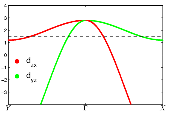
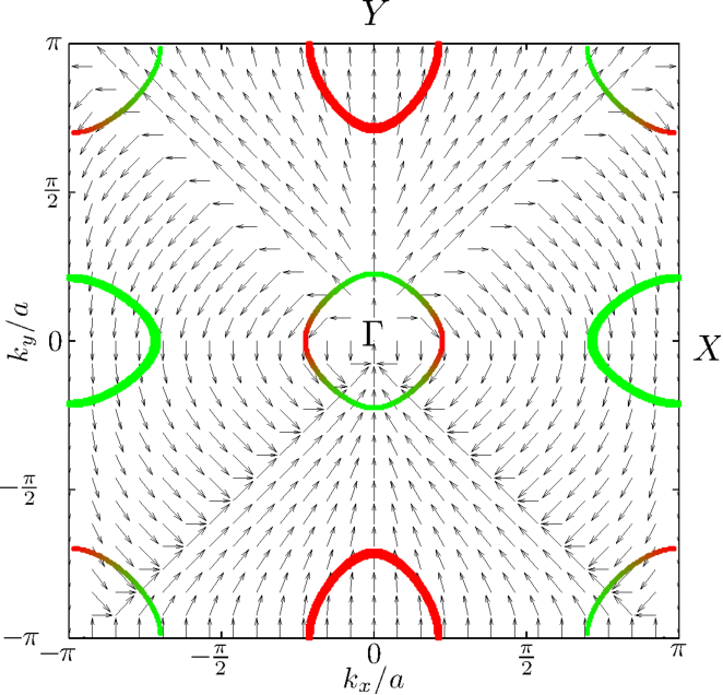
Diagonalizing the Hamiltonian we obtain two bands . A generic band structure closed to the Fermi level showing the orbital weights is represented in Fig. 2. Both orbitals contribute to the pockets while the electron pocket has dominant component. The pocket has a vortex structure as it was pointed out in Ref. [65] for the two and five orbital models of iron superconductors. We will identify the vortex in the continuum limit.
We are interested in a low energy description of the model i.e. in the behavior of around the , and points. In the continuum limit we expand to lowest order. Around the point we get:
and
This dispersion relation has vorticity equal to two (see Fig. 3) as it has been pointed out in [65]. For simplicity we assume , so that and around the dispersion relation is isotropic. Around the point we get instead
Where the coefficients show the opposite ellipticity of the e-pockets. All the coefficients and are functions of the hopping coefficients whose precise dependence is not important at this point.
In general, the Green’s function associated to the Hamiltonian (29) can be written as
| (30) |
where we fixed for simplicity . The vector is defined as , and labels the conduction () and valence () bands. We can particularize this Green’s function to each pocket. The vectors for are obtained by definitions using the low energy expansions . Within this approximation the vector field for the pocket is given by where we use . The vortex around described by is represented in Fig. 3. For the e-pockets we find instead that physically means that the orbital weight of the pocket is only from the orbital. Using that the point belongs to the valence band () and the pockets belong to the conduction () band we have
| (31a) | |||
| (31b) |
By using the definitions in Eq.s (31b) we can explicitly write down the expressions for the orbital components of the Green’s function of each pocket. It is easy to verify that for the pockets all the orbitals components vanish except the one
| (32) |
using , while for the pockets we have
| (33) | |||||
| (34) | |||||
| (35) |
with and . In the numerator of each Green’s function it is encoded the orbital content of each pocket.
The dispersion relations within this approximation can be expressed by , , is the offset energy. To better compare with previous results we treat the ellipticity perturbatively analogously to what is discussed in Ref. [44]. We assume the isotropic mass for the h-pocket as and we use the parameter encoding the ellipticity, such that the anisotropic e-pocket mass read as . Near the Fermi energy and for small ellipticity the dispersions can be approximate by and .
Magnetic Susceptibility in the Nematic Phase
In general the spin susceptibility depend on four orbital indices but in the spin-nematic scenario the spin-susceptibility, Eq.s (6-7) of the main text, depends just on two orbitals indices [76]. In the continuum limit the magnetic bubble is given by
| (36) |
where there is no summation in and we compact the notation using the quadrivectors , and . By replacing the Green’s functions by Eq. (32-35) we obtain that the only finite component is the
| (37) |
By comparison of the above equation with the expression for the bubble defined in terms of the orbital weights , Eq. (7) of the main text, we identify
| (38) |
By analogous analysis of the bubble we obtain
| (39) |
Let us focus now on the hydrodynamic limit of the static bubble Eq. (37) in the nematic phase
| (40) |
To study the –dependent part, we have to expand up to the Green’s function in Eq. (37) also taking into account the ellipticity of the pockets. The constant part and the momentum dependent one can be computed explicitly separating the momentum integral in the one over the angular variable and the other over the modulus with being the density of state at the Fermi level.
The constant part is negative and at perfect nesting diverges logarithmically as , with upper cut-off for the low-energy theory. The term is the standard logarithm appearing in the problem of the antiferromagnetic instability.
The -dependent part can be written as where
| (41) |
Thus we found that the stiffness of the magnetic bubble is anisotropic already at the level of zero ellipticity due to the angular modulation introduced by the vortex in Eq. (37). Notice that the finite term and the one proportional to have a competing role in making the magnetic stiffness anisotropic. Eq. (37) reproduces exactly the magnetic bubble obtained via orbital-less approach [44] once eliminated . The momenta analysis for this case leads to:
| (42) |
and the anisotropic stiffness is found only at order . In addition, the dependence on of the coefficients is different with respect to the one obtain retaining the orbital information, Eq.s (41) highlight that the vortex also affects the terms accounting for the ellipticity.
Notice that in the paramagnetic phase the tetragonal symmetry is respected since the anisotropic properties found for the hold for the having into account the orbital exchange i.e. and . Once is entered in the nematic phase the two modes are no longer equivalent and the momentum dependence of the spin fluctuations is actually anisotropic as we discussed above.
Quartic Coefficients
We start directly from the definition of the orbital nematic coefficients Eq. (5c) of the main text. By using the expressions Eq.s (38-39) for the orbital weights we have
| (43a) | |||
| (43b) |
Expanding in powers of and computing explicitly the integrals we obtain
| (44) |
with and () numerical factors: and . It holds . The tensor elements of the nematic coupling are finite also assuming circular pockets (i.e. ) while the first finite contribution in appears at the second order. All the others quartic coefficients , are related to the above ones by angular symmetry. It holds: , , , while all the others components are zero.
References
- [1] M. A. Tanatar, E. C. Blomberg, A. Kreyssig, M. G. Kim, N. Ni, A. Thaler, S. L. Bud’ko, P. C. Canfield, A. I. Goldman, I. I. Mazin, and R. Prozorov, Phys. Rev. B 81, 184508 (2010).
- [2] J.-H. Chu, J. G. Analytis, K. De Greve, P. L. McMahon, Z. Islam, Y. Yamamoto, and I. R. Fisher, Science 329, 824 (2010).
- [3] I. R. Fisher, L. Degiorgi, and Z. X. Shen, Rep. Prog. Phys. 74, 124506 (2011).
- [4] J. J. Ying, X. F. Wang, T. Wu, Z. J. Xiang, R. H. Liu, Y. J. Yan, A. F. Wang, M. Zhang, G. J. Ye, P. Cheng, J. P. Hu, and X. H. Chen, Phys. Rev. Lett. 107, 067001 (2011).
- [5] J.-H. Chu, H.-H. Kuo, J. G. Analytis, and I. R. Fisher, Science 337, 710 (2012).
- [6] H.-H. Kuo and I. R. Fisher, Phys. Rev. Lett. 112, 227001 (2014).
- [7] S. Jiang, H. S. Jeevan, J. Dong, and P. Gegenwart, Phys. Rev. Lett. 110, 067001 (2013).
- [8] R. M. Fernandes, L. H. VanBebber, S. Bhattacharya, P. Chandra, V. Keppens, D. Mandrus, M. A. McGuire, B. C. Sales, A. S. Sefat, and J. Schmalian, Phys. Rev. Lett. 105, 157003 (2010).
- [9] A. E. Böhmer, P. Burger, F. Hardy, T. Wolf, P. Schweiss, R. Fromknecht, M. Reinecker, W. Schranz, and C. Meingast, Phys. Rev. Lett. 112, 047001 (2014).
- [10] A. Dusza, A. Lucarelli, F. Pfuner, J.-H. Chu, I. Fisher, and L. Degiorgi, Europhys. Lett. 93, 37002 (2011).
- [11] M. Nakajima, T. Liang, S. Ishida, Y. Tomioka, K. Kihou, C. H. Lee, A. Iyo, H. Eisaki, T. Kakeshita, T. Ito, and S. Uchida, PNAS 108, 12238 (2011).
- [12] A. Dusza, A. Lucarelli, A. Sanna, S. Massidda, J.-H. Chu, I. R. Fisher, and L. Degiorgi, New J. Phys. 14, 023020 (2012).
- [13] M. Nakajima, S. Ishida, Y. Tomioka, K. Kihou, C. H. Lee, A. Iyo, T. Ito, T. Kakeshita, H. Eisaki, and S. Uchida, Phys. Rev. Lett. 109, 217003 (2012).
- [14] H. Z. Arham, C. R. Hunt, W. K. Park, J. Gillett, S. D. Das, S. E. Sebastian, Z. J. Xu, J. S. Wen, Z. W. Lin, Q. Li, G. Gu, A. Thaler, S. Ran, S. L. Bud’ko, P. C. Canfield, D. Y. Chung, M. G. Kanatzidis, and L. H. Greene, Phys. Rev. B 85, 214515 (2012).
- [15] E. C. Blomberg, M. A. Tanatar, R. M. Fernandes, I. I. Mazin, B. Shen, H.-H. Wen, M. D. Johannes, J. Schmalian, and R. Prozorov, Nat Commun 4, 1914 (2013).
- [16] C. Mirri, A. Dusza, S. Bastelberger, J.-H. Chu, H.-H. Kuo, I. R. Fisher, and L. Degiorgi, Phys. Rev. B 89, 060501 (2014).
- [17] Y. Gallais, R. M. Fernandes, I. Paul, L. Chauvière, Y. X. Yang, M. A. Méasson, M. Cazayous, A. Sacuto, D. Colson, and A. Forget, Phys. Rev. Lett. 111, 267001 (2013).
- [18] T.-M. Chuang, M. P. Allan, J. Lee, Y. Xie, N. Ni, S. L. Bud’ko, G. S. Boebinger, P. C. Canfield, and J. C. Davis, Science 327, 181 (2010).
- [19] M. P. Allan, T.-M. Chuang, F. Massee, Y. Xie, N. Ni, S. L. Bud/’ko, G. S. Boebinger, Q. Wang, D. S. Dessau, P. C. Canfield, M. S. Golden, and J. C. Davis, Nat. Phys. 9, 220 (2013).
- [20] E. P. Rosenthal, E. F. Andrade, C. J. Arguello, R. M. Fernandes, L. Y. Xing, X. C. Wang, C. Q. Jin, A. J. Millis, and A. N. Pasupathy, Nat Phys 10, 225 (2014).
- [21] S. Kasahara, H. J. Shi, K. Hashimoto, S. Tonegawa, Y. Mizukami, T. Shibauchi, K. Sugimoto, T. Fukuda, T. Terashima, A. H. Nevidomskyy, and Y. Matsuda, Nature 486, 382 (2012).
- [22] L. W. Harriger, H. Q. Luo, M. S. Liu, C. Frost, J. P. Hu, M. R. Norman, and P. Dai, Phys. Rev. B 84, 054544 (2011).
- [23] C. Dhital, Z. Yamani, W. Tian, J. Zeretsky, A. S. Sefat, Z. Wang, R. J. Birgeneau, and S. D. Wilson, Phys. Rev. Lett. 108, 087001 (2012).
- [24] Y. Song, S. V. Carr, X. Lu, C. Zhang, Z. C. Sims, N. F. Luttrell, S. Chi, Y. Zhao, J. W. Lynn, and P. Dai, Phys. Rev. B 87, 184511 (2013a).
- [25] S. Ibuka, Y. Nambu, T. Yamazaki, M. D. Lumsden, and T. J. Sato, Physica C: Superconductivity 507, 25 (2014).
- [26] X. Lu, J. T. Park, R. Zhang, H. Luo, A. H. Nevidomskyy, Q. Si, and P. Dai, Science 345, 657 (2014).
- [27] M. Yi, D. Lu, J.-H. Chu, J. G. Analytis, A. P. Sorini, A. F. Kemper, B. Moritz, S.-K. Mo, R. G. Moore, M. Hashimoto, W.-S. Lee, Z. Hussain, T. P. Devereaux, I. R. Fisher, and Z.-X. Shen, PNAS 108, 6878 (2011).
- [28] M. Yi, D. H. Lu, R. G. Moore, K. Kihou, C.-H. Lee, A. Iyo, H. Eisaki, T. Yoshida, A. Fujimori, and Z.-X. Shen, New J. Phys. 14, 073019 (2012).
- [29] Y. K. Kim, W. S. Jung, G. R. Han, K.-Y. Choi, C.-C. Chen, T. P. Devereaux, A. Chainani, J. Miyawaki, Y. Takata, Y. Tanaka, M. Oura, S. Shin, A. P. Singh, H. G. Lee, J.-Y. Kim, and C. Kim, Phys. Rev. Lett. 111, 217001 (2013).
- [30] S. Ishida, M. Nakajima, T. Liang, K. Kihou, C. H. Lee, A. Iyo, H. Eisaki, T. Kakeshita, Y. Tomioka, T. Ito, and S. Uchida, Phys. Rev. Lett. 110, 207001 (2013).
- [31] M. N. Gastiasoro, I. Paul, Y. Wang, P. J. Hirschfeld, and B. M. Andersen, Phys. Rev. Lett. 113, 127001 (2014).
- [32] Y. Wang, M. N. Gastiasoro, B. M. Andersen, M. Tomić, H. O. Jeschke, R. Valentí, I. Paul, and P. J. Hirschfeld, Phys. Rev. Lett. 114, 097003 (2015).
- [33] C. Fang, H. Yao, W.-F. Tsai, J. Hu, and S. A. Kivelson, Phys. Rev. B 77, 224509 (2008).
- [34] C. Xu, M. Müller, and S. Sachdev, Phys. Rev. B 78, 020501 (2008).
- [35] C.-C. Lee, W.-G. Yin, and W. Ku, Phys. Rev. Lett. 103, 267001 (2009).
- [36] B. Valenzuela, E. Bascones, and M. J. Calderón, Phys. Rev. Lett. 105, 207202 (2010).
- [37] Z. P. Yin and W. E. Pickett, Physical Review B 81, 174534 (2010).
- [38] W. Lv, F. Krüger, and P. Phillips, Phys. Rev. B 82, 045125 (2010).
- [39] C.-C. Chen, J. Maciejko, A. P. Sorini, B. Moritz, R. R. P. Singh, and T. P. Devereaux, Phys. Rev. B 82, 100504 (2010).
- [40] M. S. Laad and L. Craco, Phys. Rev. B 84, 054530 (2011).
- [41] A. Cano, M. Civelli, I. Eremin, and I. Paul, Phys. Rev. B 82, 020408 (2010).
- [42] A. Cano, Phys. Rev. B 84, 012504 (2011).
- [43] A. Cano and I. Paul, Phys. Rev. B 85, 155133 (2012).
- [44] R. M. Fernandes, A. V. Chubukov, J. Knolle, I. Eremin, and J. Schmalian, Phys. Rev. B 85, 024534 (2012).
- [45] R. M. Fernandes and J. Schmalian, Supercond. Sci. Technol. 25, 084005 (2012).
- [46] S. Liang, A. Moreo, and E. Dagotto, Phys. Rev. Lett. 111, 047004 (2013).
- [47] S. Liang, A. Mukherjee, N. D. Patel, E. Dagotto, and A. Moreo, arXiv:1405.6395 (2014).
- [48] I. Paul, Phys. Rev. B 90, 115102 (2014).
- [49] R. M. Fernandes, A. V. Chubukov, and J. Schmalian, Nat Phys 10, 97 (2014).
- [50] J. C. Davis and P. J. Hirschfeld, Nat Phys 10, 184 (2014).
- [51] S.-H. Baek, D. V. Efremov, J. M. Ok, J. S. Kim, J. van den Brink, and B. Büchner, Nature Materials 14, 210–214 (2015).
- [52] R. Yu, K. Trinh, A. Moreo, M. Daghofer, J. A. Riera, S. Haas, and E. Dagotto, Phys. Rev. B 79, 104510 (2009).
- [53] E. Bascones, M. J. Calderón, and B. Valenzuela, Phys. Rev. Lett. 104, 227201 (2010).
- [54] M. Daghofer, A. Nicholson, A. Moreo, and E. Dagotto, Phys. Rev. B 81, 014511 (2010).
- [55] Z. P. Yin, K. Haule, and G. Kotliar, Nature Physics 7, 294 (2011).
- [56] S. Graser, T. Maier, P. Hirschfeld, and D. Scalapino, New J. Phys. 11, 025016 (2009).
- [57] J. T. Park, D. S. Inosov, A. Yaresko, S. Graser, D. L. Sun, P. Bourges, Y. Sidis, Y. Li, J. H. Kim, D. Haug, A. Ivanov, K. Hradil, A. Schneidewind, P. Link, E. Faulhaber, I. Glavatskyy, C. T. Lin, B. Keimer, and V. Hinkov, Phys. Rev. B 82, 134503 (2010).
- [58] H. Park, K. Haule, and G. Kotliar, Phys. Rev. Lett. 107, 137007 (2011).
- [59] J. Lorenzana, G. Seibold, C. Ortix, and M. Grilli, Phys. Rev. Lett. 101, 186402 (2008).
- [60] J. Knolle, I. Eremin, A. V. Chubukov, and R. Moessner, Phys. Rev. B 81, 140506 (2010).
- [61] M. Capati, M. Grilli, and J. Lorenzana, Phys. Rev. B 84, 214520 (2011).
- [62] P. M. R. Brydon, J. Schmiedt, and C. Timm, Phys. Rev. B 84, 214510 (2011).
- [63] G. S. Tucker, R. M. Fernandes, H. F. Li, V. Thampy, N. Ni, D. L. Abernathy, S. L. Bud’ko, P. C. Canfield, D. Vaknin, J. Schmalian, and R. J. McQueeney, Phys. Rev. B 86, 024505 (2012).
- [64] X.-L. Qi, S. Raghu, C.-X. Liu, D. J. Scalapino, and S.-C. Zhang, arXiv:0804.4332.
- [65] Y. Ran, F. Wang, H. Zhai, A. Vishwanath, and D.-H. Lee, Phys. Rev. B 79, 014505 (2009).
- [66] A. Lau and C. Timm, Phys. Rev. B 88, 165402 (2013).
- [67] C. Castellani, C. R. Natoli, and J. Ranninger, Phys. Rev. B 18, 4945 (1978).
- [68] L. Fanfarillo, A. Cortijo, and B. Valenzuela, Work in progress.
- [69] S. Avci, O. Chmaissem, J. Allred, S. Rosenkranz, I. Eremin, A. Chubukov, D. Bugaris, D. Chung, M. Kanatzidis, J.-P. Castellan, J. Schlueter, H. Claus, D. Khalyavin, P. Manuel, A. Daoud-Aladine, and R. Osborn, Nature Communications 5 (2014).
- [70] M. J. Calderon, B. Valenzuela, and E. Bascones, New J. Phys. 11, 013051 (2009).
- [71] K. W. Song, Y.-C. Liang, H. Lim, and S. Haas, Phys. Rev. B 88, 054501 (2013b).
- [72] J. Negele and H. Orland, Quantum many particle system (Addison-Wesley, New York, 1988).
- [73] L. Benfatto, A. Toschi, and S. Caprara, Phys. Rev. B 69, 184510 (2004).
- [74] L. Fanfarillo, L. Benfatto, S. Caprara, C. Castellani, and M. Grilli, Phys. Rev. B 79, 172508 (2009).
- [75] M. Marciani, L. Fanfarillo, C. Castellani, and L. Benfatto, Phys. Rev. B 88, 214508 (2013).
- [76] This is a direct consequence of neglecting interorbital magnetization in the original Hamiltonian i.e. of considering in the spin-operator definition only fermions coming from the same orbital .