Tunneling through high energy barriers in simulated quantum annealing

The correspondence between minimizing a real-valued function on a discrete domain and finding the ground state which minimizes the energy of a physical system has inspired a variety of optimization methods based on physical processes. Simulated annealing (SA) is a popular classical algorithm based on a Markov chain Monte Carlo model of the thermal processes that take place in a system as it is cooled to low temperatures[1]. Quantum annealing (QA) is a more recently proposed algorithm [2], intended to run on quantum hardware, which takes advantage of the tendency for quantum systems to remain in the ground state of a time-dependent Hamiltonian that transforms sufficiently slowly. A third physics-inspired optimization method is simulated quantum annealing (SQA), which uses a Quantum Monte Carlo method [3] to sample the output distribution of a quantum annealing process on a classical computer.

One approach to understanding the strengths and weaknesses of these three optimization methods is to benchmark the performance of SA, QA, and SQA on large ensembles of random instances of NP-Hard discrete optimization problems. In [4] the success probabilities of QA and SQA are found to be highly correlated across random instances of quadratic unconstrained binary optimization on the Chimera graph, while the distribution of success probabilities for SA on the same set of instances bears little resemblance to that of QA and SQA. In [5] SQA was found to be more efficient than SA at solving random instances of 2D Ising spin glasses, but in [6] SQA performed worse than SA on hard instances of the Traveling Salesman Problem.

Rigorous comparisons of these optimization methods have also been performed on specific problem instances that can be treated analytically. In [7] several examples are given for which QA efficiently finds the minimum, but topological obstructions cause SQA to take exponential time to equilibrate. An example given in [8] called the “Hamming weight with a spike” demonstrates that QA can be exponentially faster than SA, and in this work we examine the equilibration time of SQA for this particular instance to determine whether it inherits the quantum advantage of QA or the classical defficiency of SA.

As our measure of convergence time for SQA we consider the minimum number of sweeps $\tau_{s}$ needed to sample the true minimum of $f$ with a reasonably high probability. Each sweep consists of a systematic scan of single site updates that procedes through the bits within the 1^st trotter slice, then the 2^nd trotter slice, and so on.

We decreased the transverse field geometrically along a schedule $\Gamma_{0},...,\Gamma_{m}$ with $\Gamma_{0}=1$ and $\Gamma_{i+1}=0.7\Gamma_{i}$, until reaching a final value of $\Gamma_{m}\approx 10^{-12}$. We consider system sizes up to $n=1400$, and use an inverse temperature of $\beta=32$ to ensure that the true minimum of $f$ has overwhelmingly high probability in the stationary distribution $\pi$ when $\Gamma=\Gamma_{m}$.

In many applications of SQA the trotter number $L$ is taken to be a constant that is independent of the number of quantum spins $n$. In this work, however, we find it is necessary that $L$ should scale at least linearly with $n$, so that the probability $\mathcal{O}(\exp(-\frac{\beta n}{L}))$ of accepting a bit flip which increases the number of trotter slices with Hamming weight $n/4$ is not exponentially small in $n$. If $L$ is taken to be a constant then the equilibration time will become exponential at sufficiently large values of $n$, indicating a crossover from quantum to classical behavior.

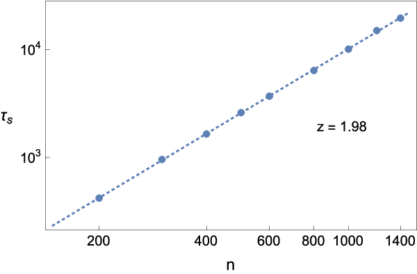
Figure 2 contains the main results of this work. We find that $\tau_{s}\approx\mathcal{O}(n^{z})$, with the dynamical critical exponent $\mathtt{z}\approx 1.98$. Since the ferromagnetic coupling in equation 2 diverges as $J=\mathcal{O}(\Gamma^{-1})$ as $\Gamma\rightarrow 0$, we can compare this with the exact value $\mathtt{z}=2$ for critical slowdown of the single site dynamics in the $\beta\rightarrow\infty$ phase transition of the 1D kinetic Ising model [11]. This is the same scaling of the convergence time as we would find without the high barrier at Hamming weight $n/4$, since then we would have $n$ uncoupled 1D Ising models with $L=\mathcal{O}(n)$ sites each (recall that we defined $\tau_{s}$ to count the number of sweeps, which accounts for the extra factor of $n$).

We present evidence that SQA can be exponentially faster than SA in minimizing an energy function with a high barrier. We further find that the equilibration time of SQA on this instance is not inhibited by the barrier at all, provided that the discretization in the imaginary-time direction is sufficiently fine. Directions for future work include finding an analytic proof of this exponential separation in algorithmic performance, as well as searching for random instances of optimization problems which have similar features in their energy landscape to further understand the conditions which make SQA useful.

We thank Aram Harrow for proposing this problem and for useful discussions. MD did this work as an intern for the Center for Excellence in Education Research Science Institute 2014 at MIT. EC was funded by NSF grant number CCF-1111382 and did this work while a visiting student at the MIT CTP.

References

- [1] Kirkpatrick, Gelatt, Vecchi Optimization by simulated annealing Science 220, 671-680 (1983).
- [2] Edward Farhi, Jeffrey Goldstone, Sam Gutmann, and Michael Sipser. Quantum computation by adiabatic evolution, 2000. arXiv:quant-ph/0001106.
- [3] Anders W. Sandvik Computational Studies of Quantum Spin Systems, 2010 AIP Conf.Proc.1297:135 arXiv:1101.3281 [cond-mat.str-el]
- [4] Sergio Boixo, Troels F. Rønnow, Sergei V. Isakov, Zhihui Wang, David Wecker, Daniel A. Lidar, John M. Martinis, Matthias Troyer Quantum annealing with more than one hundred qubits Nature Phys. 10, 218 (2014). arXiv:1304.4595 [quant-ph]
- [5] Roman Martoňák, Giuseppe E. Santoro, and Erio Tosatti Quantum annealing by the path-integral Monte Carlo method: The two-dimensional random Ising model, 2002. Physical Review B 66, 094203.
- [6] Demian Battaglia, Giuseppe Santoro, Erio Tosatti Optimization by Quantum Annealing: Lessons from hard 3-SAT cases Phys. Rev. E 71, 066707 (2005). arXiv:cond-mat/0502468 [cond-mat.dis-nn]
- [7] M. B. Hastings, M. H. Freedman. Obstructions To Classically Simulating The Quantum Adiabatic Algorithm, 2013. arXiv:1302.5733 [quant-ph].
- [8] Edward Farhi, Jeffrey Goldstone, Sam Gutmann. Quantum Adiabatic Evolution Algorithms versus Simulated Annealing, 2002. arXiv:quant-ph/0201031.
- [9] B. Reichardt The quantum adiabatic optimization algorithm and local minima Proc. 36th STOC, pages 502–510, 2004
- [10] Sergey Bravyi Monte Carlo simulation of stoquastic Hamiltonians, 2014. arXiv:1402.2295 [quant-ph]
- [11] Vladimir Privman Nonequilibrium Statistical Mechanics in One Dimension Cambridge University Press, 2005.