SN 2012ec: mass of the progenitor from PESSTO follow-up of the photospheric phase.
Abstract
We present the results of a photometric and spectroscopic monitoring campaign of SN 2012ec, which exploded in the spiral galaxy NGC 1084, during the photospheric phase. The photometric light curve exhibits a plateau with luminosity and duration 90 days, which is somewhat shorter than standard Type II-P supernovae. We estimate the nickel mass from the luminosity at the beginning of the radioactive tail of the light curve. The explosion parameters of SN 2012ec were estimated from the comparison of the bolometric light curve and the observed temperature and velocity evolution of the ejecta with predictions from hydrodynamical models. We derived an envelope mass of , an initial progenitor radius of and an explosion energy of . These estimates agree with an independent study of the progenitor star identified in pre-explosion images, for which an initial mass of was determined. We have applied the same analysis to two other type II-P supernovae (SNe 2012aw and 2012A), and carried out a comparison with the properties of SN 2012ec derived in this paper. We find a reasonable agreement between the masses of the progenitors obtained from pre-explosion images and masses derived from hydrodynamical models. We estimate the distance to SN 2012ec with the Standardized Candle Method (SCM) and compare it with other estimates based on other primary and secondary indicators. SNe 2012A, 2012aw and 2012ec all follow the standard relations for the SCM for the use of Type II-P SNe as distance indicators.
Keywords:
supernovae: general – supernovae: individual: SN 2012ec, SN 2012aw, SN 2012A – supernovae:individual:NGC10841 Introduction
Core-collapse supernovae (CC-SNe) originate from the gravitational collapse of the iron cores formed by massive stars () that cannot be supported by further exothermal thermonuclear reactions (Iben
&
Renzini 1983; Woosley et al. 2002). An important sub-class of CC-SNe is represented by Type II-plateau events (SNe II-P) characterized by the presence of hydrogen in their spectra (Filippenko, 1997) and a luminosity “plateau” that lasts for days, after the blue band maximum of the light curve (Barbon et al., 1979). The plateau is powered by the recombination of hydrogen in the SN ejecta. When the recombination ends, the lightcurve drops sharply by several magnitudes in days (e.g. Kasen
&
Woosley 2009; Olivares et al. 2010).
This transition phase is followed by a linear “radioactive tail”, where the light curve is powered by the radioactive decay of 56Co to 56Fe. In this phase the SN luminosity depends on the amount of 56Ni synthesized in the explosion (e.g. Weaver
&
Woosley 1980).
Both theoretical (e.g. Grassberg et al. 1971; Litvinova
&
Nadezhin 1983; Utrobin
&
Chugai 2008; Pumo
&
Zampieri 2011; Bersten et al. 2012) and empirical (e.g. Smartt et al. 2009) investigations show that type II-P SNe are generally associated with red supergiants (RSGs). A minor fraction of them (less than , e.g. Smartt et al. 2009; Kleiser et al. 2011; Pastorello et al. 2012) results from the explosion of a blue supergiant, similar to SN 1987A (Gilmozzi et al. 1987; Kirshner et al. 1987). Theoretical models predict that type II-P SNe are the final fate of progenitors between and (e.g. Heger et al. 2003; Walmswell
&
Eldridge 2012).
Most progenitors identified in high-resolution archival images were found to be RSGs of initial masses between and . The apparent lack of high-mass progenitors has been dubbed as the “RSG problem” (Smartt et al. 2009, and references therein).
The existence of this discrepancy has been further confirmed by studies of the massive star population in Local Group galaxies, for which RSGs have been found to have masses up to (Massey et al. 2000; Massey et al. 2001).
The reason for this lack of detection of massive RSG progenitors is still debated. A possible solution of the RSG problem was presented by Walmswell
&
Eldridge (2012). They speculate that an underestimation of the luminosity of the RSG SN progenitors (and therefore of their masses) might occur if we neglect the presence of an additional extinction due to dust production in the RSG winds. They estimated a new upper limit for the mass range of , which is, within the errors, marginally consistent with the range derived by Smartt (2009). Kochanek et al. (2012) pointed out that the use of standard interstellar extinction laws may overestimate the effects of the reddening.
A different approach to estimate the mass of Type II-P SN progenitors is based on the use of hydrodynamic modelling of the SN evolution. This allows us to determine the ejecta mass, explosion energy, pre-SN radius and Ni mass by performing a simultaneous comparison between the observed and simulated light curves, the evolution of line velocities and the continuum temperature (Litvinova
&
Nadezhin 1983; Litvinova
&
Nadezhin 1985; Zampieri 2005; Zampieri 2007).
The pre-explosion mass is calculated from the ejecta mass assuming the mass of a neutron star remnant () and mass loss through stellar winds. The hydrodynamic modelling of several well-observed Type II-P SNe (SNe 1997D, Zampieri et al. 1998; 1999em, Elmhamdi et al. 2003; 2003Z, Utrobin et al. 2007 and Spiro et al. 2014; 2004et, Maguire et al. 2010; 2005cs, Pastorello et al. 2009; 2009kf, Botticella et al. 2012) determined higher masses for the progenitors than those derived from the analysis of pre-explosion images. This discrepancy either points to systematic errors in the analysis of pre-explosion images or in the assumptions in the physiscs of the hydrodinamical modelling (Utrobin 1993; Blinnikov et al. 2000; Chugai
&
Utrobin 2000; Zampieri et al. 2003; Pastorello et al. 2004; Utrobin 2007, Utrobin et al. 2007; Utrobin
&
Chugai 2008; Utrobin
&
Chugai 2009; Pastorello et al. 2009).
Another method to estimate the mass of the progenitor is the modeling of nebular phase spectroscopic observations (Jerkstrand et al. 2012; Jerkstrand et al. 2014) ,which provide good agreement with estimates obtained by the analysis of pre-explosion images.
The astrophysical interest in Type II-P SNe is twofold: 1) observations show that Type II-P SNe are the most common explosions in the nearby Universe (e.g. Cappellaro et al. 1999; Li et al. 2011); and 2) starting from the pioneering suggestion by Kirshner & Kwan (1974), Type II-P SNe have been proposed as robust distance indicators. Two different approaches are used to derive distance measurements of SNe II-P. The theoretical approach is based on spectral modelling like the expanding photosphere method (e.g. Eastman, Schmidt & Kirshner 1996) or the spectral expanding atmosphere method (e.g., Baron et al. 2004). Empirical approaches exploit the observed correlation between the luminosity of a Type II-P SN and its expansion velocity (e.g., the standardized candle method, Hamuy & Pinto 2002) or the steepness of the light curve after the plateau phase (Elmhamdi, Chugai & Danzinger, 2003). The Hamuy & Pinto (2002) method, refined for example by Nugent et al. (2006), Poznanski et al. (2009), and Olivares et al. (2010), has an intrinsic accuracy of (Hamuy & Pinto, 2002); slightly larger than the accuracy obtained for Type Ia SNe (e.g. Tammann & Reindl 2013). Type II-P SNe can, importantly, be observed out to cosmological distances (e.g. Nugent et al. 2006); with the advantage of being that they arise from a homogenous progenitor population. The Hamuy & Pinto (2002) method can, therefore, be used as an independent health check of the SN Ia-based distance scale.
The main goal of this paper is to present the results of our photometric and spectroscopic monitoring campaign of SN 2012ec, which exploded in NGC 1084. The early data were collected via the Large Program ‘‘Supernova Variety and Nuclesosynthesis Yelds’’(PI S. Benetti). A substantial fraction of the data has been collected via the ESO Public Survey PESSTO 11 1 www.pessto.org (“Public ESO Spectroscopic Survey of Transient Objects”, PI S.J. Smartt). The observations of SN 2012ec were analysed in conjunction with the hydrodynamical codes described in Pumo et al. (2010) and Pumo & Zampieri (2011), and information on the progenitor obtained from high-resolution pre-explosion images. The same analysis has already performed for two other type II-P SNe: SN 2012A (Tomasella et al. 2013; Roy et al. 2014) and SN 2012aw (Fraser et al. 2012; Bayless et al. 2013; Bose et al. 2013; Dall’Ora et al. 2014). This allows us to carry out an homogeneous comparative study of these three SNe, and to identify possible systematic discrepancies in the estimates of the masses of the progenitors derived from different techniques.
The paper is organized as follows: in Section 2 we present the discovery and the detection of the progenitor of SN 2012ec; in Section 3 we discuss the properties of the host galaxy, the distance and the extinction; in Section 4 we present the optical and near-infrared (NIR) photometric evolution of SN 2012ec, and compare its colour evolution and bolometric light curve with those of other Type II-P SNe. In Section 5 we present the optical and NIR spectroscopic observations. In Section 6 we discuss the results of the modeling of the data and in Section 7 we present a detailed comparison of SN 2012ec with the Type II-P SNe 2012A and 2012aw. In Section 8 we consider these three SNe in the context of the SCM and in Section 9 we discuss our results.
2 Discovery and progenitor detection
SN 2012ec was discovered by Monard (2012) in the almost face-on (, Moiseev 2000) spiral galaxy NGC 1084 on 2012 August 11.039 UT (MJD=56150.04). Childress et al. (2012) classified SN 2012ec as a very young type II-P SN, probably a few days post-explosion. In Fig. 1 we show this early spectrum of SN 2012ec (collected on 2012, August 13 with WiFeS, MJD ), compared with SN 2006bp (Quimby et al., 2007) at five different epochs. The spectrum of SN 2012ec is very similar to those of SN 2006bp (Quimby et al., 2007) obtained at and days after the explosion, implying that the SN was observed at days post-explosion and giving an explosion epoch of days before the discovery. We explicitly note that our estimate is slightly different from the one given by Maund et al. (2013), who estimated the explosion date at days before the discovery by comparison with spectra of SN 1999em. The explosion epoch of SN 2006bp is much more tightly constrained than that of SN 1999em, because it is based on the detection of shock breakout (Nakano 2006; Quimby et al. 2007). The estimates obtained by using either SN 2006bp or SN 1999em, as reference, are in agreement within the errors. We adopt, therefore, a conservative constraint on the explosion date of days prior to discovery and define the zero phase as our estimated explosion epoch of MJD .
Maund et al. (2013) identified a progenitor candidate in pre-explosion Hubble Space Telescope (HST) images. Photometry of the progenitor candidate was compared with synthetic photometry of MARCS spectral energy distributions (SED) (Gustafsson et al., 2008), which suggested that the progenitor of SN 2012ec was a RSG with an initial mass in the range .

3 Host galaxy, distance and extinction
The SN is located E and N of the nucleus of the host galaxy NGC 1084 (see Fig 2). Details of NGC 1084 are presented in Table 1. NGC 1084 previously hosted known SNe: the Type II-P SN 2009H (Li et al., 2009), the Type II SNe 1998dl (King et al., 1998) and 1996an (Nakano et al., 1996), and the Type Ia SN 1963P (Kowal, 1968).
The distances available in the literature for NGC 1084 are principally based on the Tully-Fisher relation, and we adopt the value mag, available in the Extragalactic Distance Database 22 2 Extragalactic Distance Database, http://edd.ifa.hawaii.edu/ (Tully et al., 2009).
The Galactic reddening towards SN 2012ec was estimated from the Schlafly & Finkbeiner (2011) dust maps to be mag33 3 We checked the consistency with the Schlegel et al. (1998) calibration, and they agree within a few thousandths of magnitude . The internal reddening in NGC 1084 was derived using the measured equivalent widths (EW) of NaI D (, Å), observed in a low-resolution spectrum at days. The measured value was Å from which we obtained mag using the Poznanski et al. (2012) calibration and mag using the Turatto et al. (2003) calibration. These two values are in good agreement and we adopt mag for the host galaxy reddening.
Assuming a Cardelli et al. (1989) reddening law (), we estimate the total Galactic and host band extinction towards SN 2012ec to be mag.
| (2000) | |
|---|---|
| (2000) | |
| morphological type | SA(s)d |
| z | |
| mag | |
| vHel | |
| mag | |
| mag |
4 Photometric evolution
4.1 Data sample and reduction
A photometric and spectroscopic monitoring campaign for SN 2012ec, at optical and NIR wavelengths, was conducted over a period days, covering epochs from to days post-explosion, using multiple observing facilities. Additional data collected in the nebular phase will be published in a companion paper (Jerkstrand et al. 2014, subm.).
Johnson-Cousins data were collected with: the m Liverpool Telescope (LT, Canary Islands, Spain) equipped with the IO:O camera (, epochs); the m ESO New Technology Telescope (NTT, La Silla, Chile) equipped with the EFOSC2 (ESO Faint Object and Spectrograph Camera) camera (, epochs); the m Copernico telescope (Asiago, Italy) equipped with the AFOSC Asiago Faint Object Spectrograph and Camera (; epochs); the m ESO TRAnsiting Planets and PlanetesImals Small Telescope (TRAPPIST, La Silla, Chile), equipped with TRAPPISTCAM (, epochs); and the the array of m Panchromatic Robotic Optical Monitoring and Polarimetry Telescopes (PROMPT, Cerro Tololo, Chile), equipped with Apogee U47p cameras, which employ the E2V CCDs (, epochs).
images were collected with: the LT equipped with the IO:O camera ( epochs); the ESO NTT Telescope equipped with EFOSC2 (, epochs); the PROMPT telescopes (, epochs); and the m telescope at the Wendelstein Observatory (Mount Wendelstein, Germany), equipped with a ST-10 CCD camera (, epochs).
observations were acquired with the ESO NTT telescope, equipped with the SOFI (Son Of ISAAC) camera ( epochs).
A summary of the characteristics of the instruments and telescopes used for photometric follow up are presented in Table 2.
| Telescope | Camera | Pixel scale | Field of view | Filtersa | # of epochs |
|---|---|---|---|---|---|
| [arcsec/pix] | [arcmin] | ||||
| NTT (3.58m) | EFOSC2 | 0.24 | 4 4 | ; | 12 |
| NTT (3.58m) | SOFI | 0.28 | 5 5 | 8 | |
| LT (2.0m) | IO:O | 0.15 | 10 10 | : | 21 |
| PROMPT (0.41m) | APU9 | 0.59 | 11 11 | ; | 21 |
| CAO (1.82m) | AFOSC | 0.46 | 8 8 | ; | 3 |
| SAO (0.97m) | SBIG | 0.86 | 57 38 | 1 | |
| WOT (0.4m) | SBIG ST-10 XME | 0.44 | 16 10 | 7 | |
| TRAPPIST (0.60m) | TRAPPISTCAM | 0.65 | 27 27 | , , | 4 |
NTT = New Technology Telescope with the optical camera ESO Faint Object Spectrograph and Camera EFOSC2 and with the Near-Infrared Camera Son of ISAAC (SOFI); LT = the Liverpool Telescope (LT) with the optical CCD CAMERA IO:O; PROMPT = Panchromatic Robotic Optical Monitoring and Polarimetry Telescopes; CAO = the Copernico telescope at Asiago Observatory with the Asiago Faint Object Spectrograph and Camera (AFOSC); SAO = the Schmidt telescope at the Asiago Observatory; WOT = the telescope at the Wendelstein Observatory; TRAPPIST = TRAnsit Planets and PlanetesImals Small Telescope.
a The NTT and CAO i filter is Gunn.
Data were pre-reduced using the respective instrument pipelines, where available, or following the standard procedures (bias, overscan and flat-field corrections, trimming) in the IRAF 44 4 IRAF is distributed by the National Optical Astronomical Observatory, which is operated by the Association of Universities for Research in Astronomy, Inc., under cooperative agreement with the National Science Foundation. environment. In particular, NIR images were pre-reduced by means of an IRAF-based custom pipeline based on the XDIMSUM IRAF package (Coppola et al., 2011), which conducts the background subtraction using a two-step technique based on a preliminary guess of the sky background and with a careful masking of unwanted sources in the sky images.
Johnson-Cousins calibrated magnitudes of reference stars were obtained by averaging their photometry obtained on photometric nights, in conjunction with observations of Landolt (1992) standard star fields. calibrated photometry for reference stars were obtained on photometric nights with the LT and the NTT telescopes, in conjunction with observations of Smith et al. (2002) standard star fields. Finally, calibrated NIR 2MASS photometry was obtained for reference stars, for which 2MASS (Skrutskie et al., 2006) photometry was available. We did not correct NIR magnitudes for colour terms, since they are generally very small in the NIR bands (e.g. Carpenter 2001). Our adopted reference stars showed no clear signs of variability.
The host galaxy and the SN position are shown in Fig. 2, along with the local sequence stars adopted for the photometric calibration. The calibrated photometry for the local sequence stars is reported in Tables 3 and 4. In the following, the Johnson-Cousins and NIR photometry are reported in Vega magnitudes, while the photometry is reported in the AB magnitude system.

.
| # id | |||||||||||
|---|---|---|---|---|---|---|---|---|---|---|---|
| (deg) | (deg) | mag | mag | mag | mag | mag | mag | mag | mag | mag | |
| 1 | 41.5216674 | -7.5597940 | 17.98 (0.02) | 16.88 (0.02) | 16.19 (0.02) | 15.53 (0.03) | 19.85 (0.02) | 17.48 (0.04) | 16.41 (0.01) | 16.01 (0.02) | 15.86 (0.01) |
| 2 | 41.5496917 | -7.6416869 | 16.84 (0.02) | 15.97 (0.02) | 15.46 (0.02) | 14.93 (0.03) | 18.27 (0.02) | 16.43 (0.02) | 15.67 (0.02) | 15.38 (0.01) | 15.32 (0.02) |
| 3 | 41.5474764 | -7.6530580 | 17.14 (0.02) | 16.28 (0.02) | 15.81 (0.02) | 15.32 (0.02) | 18.45 (0.06) | 16.71 (0.03) | 16.04 (0.02) | 15.78 (0.01) | 15.72 (0.01) |
| 4 | 41.5265649 | -7.6778087 | 15.58 (0.02) | 14.95 (0.02) | 14.66 (0.02) | 16.48 (0.03) | 15.25 (0.02) | 14.80 (0.02) | 14.64 (0.02) | 14.65 (0.01) | |
| 5 | 41.5589242 | -7.6811761 | 14.27 (0.02) | 13.52 (0.02) | 13.23 (0.02) | 15.18 (0.02) | 13.91 (0.02) | 13.31 (0.02) | 13.05 (0.02) | 12.94 (0.01) | |
| 6 | 41.5522025 | -7.6973300 | 17.01 (0.02) | 16.00 (0.02) | 15.43 (0.02) | 18.82 (0.05) | 16.55 (0.03) | 15.62 (0.02) | 15.30 (0.02) | 15.18 (0.01) | |
| 7 | 41.5886692 | -7.5829251 | 14.62 (0.01) | 14.07 (0.01) | 13.84 (0.02) | 15.36 (0.03) | 14.49 (0.02) | 13.98 (0.01) | 13.86 (0.02) | 13.87 (0.01) | |
| 9 | 41.6065545 | -7.5858940 | 15.16 (0.01) | 14.42 (0.01) | 14.08 (0.02) | 16.11 (0.02) | 15.03 (0.03) | 14.25 (0.02) | 14.04 (0.02) | 14.01 (0.01) | |
| 11 | 41.6108998 | -7.5996059 | 16.99 (0.01) | 16.36 (0.01) | 16.04 (0.02) | 17.64 (0.02) | 16.66 (0.03) | 16.21 (0.01) | 15.99 (0.02) | 15.97 (0.02) | |
| 12 | 41.5528922 | -7.5585795 | 18.32 (0.02) | 16.83 (0.02) | 15.93 (0.02) | 14.73 (0.02) | 20.12 (0.05) | 17.65 (0.01) | 16.19 (0.01) | 15.24 (0.02) | 14.90 (0.02) |
| 16 | 41.5215760 | -7.5167457 | 16.06 (0.01) | 15.26 (0.01) | 14.90 (0.02) | 14.48 (0.01) | 17.25 (0.04) | 15.64 (0.03) | 15.10 (0.02) | 14.93 (0.02) | 14.86 (0.01) |
| 17 | 41.4300180 | -7.5076398 | 14.74 (0.01) | 14.08 (0.01) | 13.81 (0.02) | 14.92 (0.02) | 14.43 (0.02) | 14.18 (0.02) | 13.92 (0.01) | 13.95 (0.01) | |
| 18 | 41.5925440 | -7.5310037 | 16.06 (0.01) | 13.76 (0.01) | 14.90 (0.02) |
| Star ID | |||||
|---|---|---|---|---|---|
| (deg) | (deg) | (mag) | (mag) | (mag) | |
| 1 | 41.5216674 | -7.5597940 | 14.82 (0.04) | 14.08 (0.05) | 13.94 (0.05) |
| 2 | 41.5496917 | -7.6416869 | 14.32 (0.03) | 13.87 (0.04) | 13.73 (0.05) |
| 3 | 41.5474764 | -7.6530580 | 14.71 (0.04) | 14.35 (0.05) | 14.14 (0.06) |
| 12 | 41.5528922 | -7.5585795 | 13.63 (0.03) | 13.01 (0.03) | 12.81 (0.03) |
Photometric measurements were carried out with the QUBA pipeline (Valenti et al., 2011), which performs DAOPHOT-based (Stetson, 1987) point-spread-function (PSF) fitting photometry on the SN and on the selected reference stars. Since SN 2012ec is embedded in a spiral arm of the host galaxy, the background was estimated with a polynomial model. We performed empirical tests for the best background subtraction, and in most cases we found that a -order polynomial model of the background gave satisfactory results, due to the high S/N ratio of the SN in these images. Only at the last few epochs was the S/N ratio of the SN too low to prohibit satisfactory removal of the local background. We note, however, that even using the subtraction of a template image would probably not yield a significant improvement, as in these cases the flux of the SN was only few tens of counts above the local background. Photometric uncertainties were automatically estimated by the pipeline using artificial star experiments.
The photometric measurements of the SN in the , and in the filter systems are reported in Table 5.
| Date | |||||||||||||
|---|---|---|---|---|---|---|---|---|---|---|---|---|---|
| (mag) | (mag) | (mag) | (mag) | (mag) | (mag) | (mag) | (mag) | (mag) | (mag) | (mag) | (mag) | ||
| 20120814 | 56154.22 | 14.99 (0.02) | 14.81 (0.02) | 15.02 (0.04) | 14.78 (0.02) | 14.91 (0.02) | |||||||
| 20120815 | 51155.22 | 14.99 (0.04) | 14.86 (0.04) | 15.09 (0.02) | 14.81 (0.02) | 14.91 (0.02) | |||||||
| 20120817 | 56157.59 | 15.12 (0.06) | 14.90 (0.06) | 14.74 (0.06) | 14.55 (0.05) | ||||||||
| 20120818 | 56158.23 | 15.10 (0.03) | 14.87 (0.03) | 15.28 (0.05) | 14.82 (0.01) | 14.94 (0.01) | |||||||
| 20120819 | 56158.34 | 15.15 (0.06) | 14.95 (0.05) | 14.73 (0.06) | 14.53 (0.03) | 14.84 (0.05) | 14.86 | ||||||
| 20120820 | 56159.31 | 15.29 (0.05) | 14.92 (0.04) | 14.62 (0.05) | 14.53 (0.05) | 15.05 (0.07) | 14.78 (0.03) | 14.86 (0.06) | |||||
| 20120821 | 56160.30 | 15.18 (0.07) | 14.86 (0.06) | 14.65 (0.03) | (14.61 (0.06) | 15.13 (0.10) | 14.81 (0.04) | 14.89 (0.04) | 14.92 (0.05) | ||||
| 20120826 | 56165.28 | 15.47 (0.05) | 14.93 (0.04) | 14.64 (0.04) | 16.35 (0.04) | 15.25 (0.08) | 14.80 (0.03) | 14.87 (0.03) | 14.92 (0.03) | 14.24 (0.02) | 14.04 (0.02) | 13.91 (0.02) | |
| 20120828 | 56168.20 | 15.55 (0.02) | 15.02 (0.02) | 16.52(0.06) | 14.85 (0.02) | 14.93 (0.02) | |||||||
| 20120831 | 56171.08 | 15.67 (0.06) | 14.98 (0.06) | 16.69 (0.08) | 14.81 (0.02) | 14.94 (0.02) | |||||||
| 20120902 | 56173.09 | 15.76 (0.04) | 14.99 (0.04) | 16.98 (0.06) | 14.85(0.02) | 14.92 (0.02) | |||||||
| 20120905 | 56176.13 | 15.76 (0.04) | 15.00 (0.05) | 14.65 (0.06) | 14.62 (0.06) | 17.05 (0.07) | 14.84 (0.03) | 14.86 (0.03) | 14.89 (0.03) | ||||
| 20120909 | 56179.34 | 15.90 (0.06) | 15.10 (0.06) | 14.78 (0.04) | 14.45 (0.02) | 15.54 (0.02) | 14.92 | 14.11 (0.03) | 13.89 (0.03) | 13.82 (0.03) | |||
| 20120910 | 56180.92 | 15.95 (0.04) | 15.14 (0.03) | 14.76 (0.01) | 14.51 (0.01) | ||||||||
| 20120911 | 56181.59 | 16.05 (0.02) | 15.15 (0.02) | 14.79 (0.03) | 14.53 (0.03) | ||||||||
| 20120916 | 56186.20 | 16.06 (0.07) | 15.10 (0.06) | 14.75 (0.04) | 14.49 (0.02) | 15.51 (0.04) | 14.89 (0.04) | 14.87 (0.02) | 14.85 (0.03) | ||||
| 20120920 | 56190.24 | 15.12 (0.03) | 14.42 (0.05) | 14.89 (0.03) | 14.85 (0.03) | 14.87 (0.03) | |||||||
| 20120923 | 56194.87 | 16.15 (0.02) | 15.10 (0.02) | 14 78 (0.01) | 14.45 (0.01) | ||||||||
| 20120924 | 56195.23 | 14.08 (0.03) | 13.89 (0.03) | 13.75 (0.03) | |||||||||
| 20120926 | 56196.20 | 16.16 (0.06) | 15.00 (0.05) | 14.72 (0.03) | 17.96 (0.09) | 15.56 (0.03) | 14.81 (0.03) | 14.81 (0.03) | 14.78 (0.03) | ||||
| 20120929 | 56199.29 | 15.02 (0.03) | 14.74 (0.03) | 14.36 (0.01) | 14.88 (0.02) | 14.81 (0.02) | 14.79 (0.02) | ||||||
| 20121001 | 56202.01 | 16.19 (0.05) | 15.11 (0.05) | 17.98 (0.11) | 14.89 (0.02) | 14.80 (0.03) | 14.82 (0.02) | ||||||
| 20121002 | 56202.20 | 16.28 (0.04) | 15.04 (0.04) | 14.74 (0.04) | 14.40 (0.02) | 15.61 (0.06) | 14.93 (0.05) | 14.84 (0.04) | 14.85 (0.04) | ||||
| 20121004 | 56204.21 | 16.33 (0.04) | 15.12 (0.03) | 14.73 (0.03) | 14.43 (0.02) | 18.07 (0.14) | 15.71 (0.04) | 14.90 (0.03) | 14.84 (0.02) | 14.84 (0.02) | |||
| 20121007 | 56208.04 | 16.23 (0.08) | 15.11 (0.08) | 18.07 (0.18) | 14.85 (0.02) | 14.78 (0.02) | 14.81 (0.03) | ||||||
| 20121010 | 56211.05 | 16.35 (0.04) | 15.16 (0.04) | 18.26 (0.10) | 15.68 (0.03) | 14.89 (0.01) | 14.83 (0.01) | 14.85 (0.02) | |||||
| 20121012 | 56212.19 | 16.46 (0.06) | 15.22 (0.07) | 14.78 (0.03) | 14.41 (0.02) | 14.94 (0.02) | 14.79 (0.03) | 14.87 (0.03) | |||||
| 20121016 | 56216.35 | 14.05 (0.03) | 13.80 (0.03) | 13.59 (0.03) | |||||||||
| 20121017 | 56217.15 | 16.50 (0.07) | 15.22 (0.06) | 14.95 (0.03) | 14.89 (0.03) | 14.77 (0.04) | |||||||
| 20121019 | 56220.42 | 16.63 (0.05) | 15.28 (0.05) | 14.77 (0.04) | 14.41 (0.03) | ||||||||
| 20121020 | 56221.06 | 16.58 (0.03) | 15.36 (0.03) | 14.8 (0.1) | 14.43 (0.02) | 18.68 (0.08) | 14.96 (0.02) | 14.86 (0.02) | 14.92 (0.02) | ||||
| 20121022 | 56223.52 | 15.00 (0.02) | 14.85 (0.03) | ||||||||||
| 20121024 | 56226.45 | 15.99 (0.06) | 15.01 (0.02) | 14.91 (0.03) | |||||||||
| 20121101 | 56232.13 | 16.79 (0.09) | 15.47 (0.08) | 14.95 (0.04) | 14.59 (0.02) | 16.00 (0.06) | 15.15 (0.03) | 15.05 (0.03) | |||||
| 20121106 | 56237.12 | 15.63 (0.03) | 15.04 (0.03) | 14.67 (0.03) | 16.2 (0.1) | 15.26 (0.02) | 15.15 (0.02) | 15.16 (0.02) | 14.35 ( 0.06) | 14.12 (0.06) | 14.04 (0.04) | ||
| 20121111 | 56242.13 | 17.1 (0.1) | 15.85 (0.08) | 15.26 (0.03) | 14.85 (0.03) | 16.38 (0.06) | 15.39 (0.02) | 15.29 (0.02) | 15.26 (0.03) | ||||
| 20121114 | 56245.20 | 14.58 (0.03) | 14.34 (0.03) | 14.28 (0.03) | |||||||||
| 20121115 | 56246.96 | 17.4 (0.1) | 16.09 (0.10) | 15.63 (0.02) | 15.47 (0.02) | 15.43 (0.02) | |||||||
| 20121117 | 56248.14 | 16.26 (0.04) | 15.57 (0.05) | 15.15 (0.04) | |||||||||
| 20121119 | 56250.19 | 17.82 (0.09) | 16.49 (0.08) | 15.85 (0.05) | 15.37 (0.05) | 17.24 (0.05) | 16.00 (0.02) | 15.89 (0.02) | 15.74 (0.03) | ||||
| 20121122 | 56253.08 | 17.95 (0.10) | 17.16 (0.10) | 16.36 (0.07) | 15.63 (0.05) | 17.45 (0.10) | 16.32 (0.03) | 16.29 (0.03) | 16.12 (0.12) | ||||
| 20121204 | 56266.14 | 15.73 (0.06) | 15.27 (0.08) | 15.40 (0.06) | |||||||||
| 20121205 | 56266.93 | 18.5 (0.2) | 17.3 (0.2) | 16.65 (0.07) | 16.51 (0.07) | 16.40 (0.06) | |||||||
| 20121207 | 56268.94 | 18.60 (0.15) | 17.40 (0.15) | 16.80(0.1) | 16.6 (0.1) | 16.50 (0.06) | |||||||
| 20121209 | 56270.95 | 18.70 (0.13) | 17.50 (0.13) | 16.9 (0.1) | 16.7 (0.1) | 16.6 (0.1) | |||||||
| 20121216 | 56277.99 | 17.0 (0.1) | 16.9 (0.1) | 16.8 (0.1) | |||||||||
| 20121220 | 56282.94 | 18.8 (0.2) | 17.7 (0.2) | 16.9 (0.2) | |||||||||
| 20121221 | 56283.10 | 15.83 (0.03) | 15.41 (0.03) | 15.47 (0.03) | |||||||||
| 20121228 | 56290.00 | 19 (0.2) | 17.9 (0.2) | 17.1 (0.1) | 17.1 (0.1) | 16.9 (0.1) | |||||||
| 20130110 | 56302.81 | 19.15 (0.30) | 18.0 (0.3) | 17.2 (0.1) | 17.2 (0.1) | 17.0 (0.1) | |||||||
| 20130112 | 56305.66 | 18.0 (0.3) | 17.15 (0.30) | 16.75 (0.30) |
4.2 Data analysis
The photometric evolution of SN 2012ec in the , and in the filter systems is shown in Fig. 3.


SN 2012ec was already on the plateau in the and bands by days. The average absolute magnitude, in the different bands, during the plateau phase was mag, mag, mag, mag, mag and mag. Using the definition for the plateau duration proposed by Olivares et al. (2010), where the end of the plateau occurs at the knee of the light curve, we found that the plateau of SN 2012ec lasted almost days in and almost days in . This is shorter than the usual duration of the plateau of standard Type II-P SNe (e.g. SN 2004et, days, Maguire et al. 2010; SN 2012aw, days, Dall’Ora et al. 2014; see also Arcavi et al. 2012). SN 2012ec began to fall from the plateau at , while the photospheric phase from the observed spectroscopic evolution (see Sect. 5.2) lasted until days. The decline in the light curve of SN 2012ec, from the plateau to the radioactive decay tail, lasted days, decreasing mag in bands, mag in the bands and mag in the band. A list of the main characteristics of the light curve, for each filter, is reported in Table 6.
| V | R | I | J | H | K | ||||
|---|---|---|---|---|---|---|---|---|---|
| mag | mag | mag | mag | mag | mag | mag | mag | mag | |
| m | 15.10 (0.02) | 14.78 (0.01) | 14.45 (0.01) | 14.89 (0.03) | 14.85 (0.03) | 14.87 (0.03) | 14.08 (0.03) | 13.89 (0.03) | 13.75 (0.03) |
| M | -16.54 (0.17) | -16.75 (0.17) | -16.96 (0.17) | -16.80 (0.18) | -16.93 (0.18) | -17.08 (0.18) | -17.24 (0.18) | -17.38 (0.18) | -17.49 (0.18) |
a Plateau phase refers to 59 days after the explosion at
The NIR light curve exhibits a plateau of duration days, which subsequently drops over a period of days by mag in the band, mag in the band and mag in the band. This behaviour is similar to that observed for other Type II-P SNe (see for example, SN 2012A, Tomasella et al. 2013; SN 2012aw Dall’Ora et al. 2014).
The evolution of the , and colours of SN 2012ec are shown in Fig. 4. The colour becomes progressively redder over the first days, rising from to , before reaching a constant value by . The colour starts from mag and increases slowly to mag at days, before increasing further from to mag in the period days. The colour evolution of SN 2012ec is similar to those of other type II-P SNe (e.g. SN 2004et, Maguire et al. 2010; SN 1999em, Elmhamdi et al. 2003; SN 2009bw, Inserra et al. 2012). The trends in the colour evolution are similar to those observed by Faran et al. 2014, see their Fig. 10 for a sample of 23 type II-P SNe.

4.3 Bolometric light curve and mass
A pseudo-bolometric light curve was calculated by integrating over the optical and NIR photometry. The apparent magnitudes have been converted into monochromatic fluxes at the effective wavelength for each filter, and then corrected for extinction (Sect. 3). The resulting SED was integrated over the entire wavelength range, assuming zero flux at the limits. The estimation of the flux was performed at only those phases for which V band observations were available. If photometry for other bands was not available, the magnitudes were estimated at these phases by interpolating the values from photometry acquired on adjacent nights. The final integrated fluxes were converted to luminosity through application of the adopted distance modulus. The pseudo-bolometric light curve of SN 2012ec is shown in Fig. 5. The luminosity at the first epoch for which the calculation could be conducted ( days) was ; this can be considered a lower limit for the bolometric luminosity. The SN luminosity reaches the plateau by day (), which then begins to significantly decrease at days to the tail at day , with a luminosity of .
A comparison of the pseudo-bolometric light curve of SN 2012ec with other Type II-P SNe demonstrates a similar behaviour (e.g. SN 2012A, Tomasella et al. 2013; SN 2012aw, Dall’Ora et al. 2014; SN 2009kf, Botticella et al. 2012; and SN 2005cs, Pastorello et al. 2009). From the pseudo-bolometric light curve of SN 2012ec, it is evident that its luminosity on the plateau is lower than observed for SNe 2012aw and SN 2009kf and that plateau duration is shorter than the more luminous SNe. SN 2012ec is more luminous than SN 2012A and SN 2005cs but has a behaviour more similar to SN 2012A. They have comparable plateau, even if the one of SN 2012A is a bit shorter. Instead SN 2005cs shows a different evolution of the light curve compared to SN 2012ec, especially the fall from the plateau that is longer for SN 2005cs.

We estimated the mass synthesised during the explosion, by comparing the luminosity of SN 2012ec with that of SN 1987A at similar late epochs. Assuming a similar -ray deposition fraction, the mass of was calculated using the relation of Bouchet et al. (1991):
| (1) |
For the mass of SN 1987A we adopted the weighted mean of the values reported by Arnett & Fu (1989) and Bouchet et al. (1991), and for the bolometric luminosity we adopted the value of Bouchet et al. (1991) (see also Suntzeff et al. 1988). For SN 2012ec we calculated , which is an average of the estimates made at , and days (the reported uncertainty is the dispersion of the values computed at each epoch). The slope of the light curve in the last epochs of the dataset is , in agreement with the rate of decay. The data from the nebular phase are published in a companion paper (Jerkstrand et al. 2014, submitted). Jerkstrand et al. (2014) estimate the nickel mass from photometry at 187 and 202 days, finding a value of , which is in good agreement with our estimate.
The evolution of the SED of SN 2012ec, based on optical and NIR photometry, is shown in Fig. 6. The observations covered the wavelength range Å. We evaluated the evolution of the SED and calculated blackbody continuum fits at each epoch. At days, the best fit gives a blackbody temperature of K, which decreases to K by day . At early time, the fits were conducted using all available photometric observations. At later epochs, the bluest photometric observations were excluded from the fits as metal line blanketing, particularly due to Fe II and Ti II, at these wavelengths caused significant departures from the ideal black body assumption (Dessart & Hillier, 2005). The u band data was excluded from the fits for data after and, in addition, the B and g bands were excluded from fits for data after .

From the blackbody fit it was possible to evaluate the time evolution of the photospheric temperature of SN 2012ec. The temperature drops rapidly in the first days from K to K, before decreasing slowly from K to K. The values of the temperature estimated from the blackbody fits to the photometric data are in good agreement with those derived from fits of the continuum in the observed spectra (within the uncertainties) from . During the first days the spectroscopic temperature varies from K to K, decreasing to at days before reaching K in the last epochs. The slightly higher temperatures estimated from the spectra are due to the limited spectroscopic wavelength range ( Å) used for the continuum fits, compared to the wavelength range covered by the available photometric data. We compared the estimated temperatures with those of SNe 2009bw (Inserra et al., 2012) and 1999em (Elmhamdi et al., 2003). SN 2012ec is cooler at earlier phases, compared to SN 2009bw which had an initial temperature of K and SN 1999em which had a temperature of K. At later pahases, the temperatures of all three SNe converge to K.
5 Spectroscopic evolution
5.1 Data sample and reduction
As a PESSTO follow-up target, SN 2012ec was scheduled for a dense spectroscopic monitoring campaign at the ESO NTT at La Silla, Chile. Ten epochs of optical spectroscopy were acquired with EFOSC2 and ten epochs of NIR spectroscopy were acquired with SOFI. The optical dataset was supplemented with spectra from the following facilities: the m telescope of the Siding Spring Observatory (SSO, New South Wales, Australia) equipped with the Wide Field Spectrograph WiFeS ( epochs), the m Nordic Optical Telescope (NOT, Canary Islands, Spain) equipped with the Andalucia Faint Object Spectrograph and Camera (ALFOSC) ( epoch), the 1.82m Copernico Telescope (Asiago, Italy) equipped with AFOSC ( epochs), the William Herschel Telescope (WHT, Canary Islands, Spain) equipped with the Intermediate dispersion Spectrograph and Imaging system (ISIS) ( epoch), the 1.22m Galileo Telescope (Asiago, Italy) equipped with the Boller Chivens spectrograph (BC) ( epochs). The spectroscopic observations cover epochs from day to day . Details of the spectroscopic observations and the characteristics of the instruments used are listed in Table 7.
| Telescope | Instrument | Grism | Range | Resolution | # of epochs |
|---|---|---|---|---|---|
| [ Å ] | [ Å ] | ||||
| NTT (3.58m) | EFOSC2 | Gr11, Gr16 | 3350-10000 | 12 | 10 |
| NTT (3.58m) | SOFI | GB | 9400-14000 | 20 | 7 |
| NTT (3.58m) | SOFI | GB, GR | 14000-25000 | 20 | 3 |
| CAO (1.82m) | AFOSC | Gr4 | 3500-8200 | 24 | 3 |
| Pennar (1.22m) | BC | Gr300 | 3400-7800 | 10 | 2 |
| NOT (2.56m) | ALFOSC | Gr4 | 3400-9000 | 14 | 1 |
| WHT (4.2m) | ISIS | R300B+R158R | 3500-10000 | 5 | 1 |
| ANU (2.3m) | WiFeS | B+R | 3300-9000 | 2 | 2 |
NTT = New Technology Telescope with the optical camera ESO Faint Object Spectrograph and Camera EFOSC2 and with the Near-Unfrared Camera Son of ISAAC (SOFI); CAO = the Copernico telescope at Asiago Observatory with the Asiago Faint Object Spectrograph and Camera (AFOSC); Pennar = Galileo telescope at Asiago Observatory with the Boller Chivens spectrograph; NOT = Nordic Optical Telescope with the Andalucia Faint Object Spectrograph and Camera (ALFOSC); WHT = William Herschel Telescope with the Intermediate dispersion Spectrograph and Imaging System (ISIS); ANU = Australian National University telescope with the Wide-Field Spectrograph (WiFeS).
Spectra were pre-reduced (trimmed, overscan, bias and flat-field corrected) using the PESSTO pipeline (Smartt et al. 2014, submitted), based on the standard IRAF tasks 55 5 Fast reduction data are available on WISeREP (Yaron & Gal-Yam, 2012) and full reduced data can be accessed from the ESO Phase 3 archive, all details on www.pessto.org. The wavelength calibration was performed using comparison spectra of arc lamps acquired with the same instrumental configuration as the SN observations. The science observations were flux calibrated with respect to observations of spectrophotometric standard stars. Further corrections for atmospheric extinction were applied using tabulated extinction coefficients for each telescope site (in the pipeline archive).
The quality of the flux calibration was checked by comparison of synthetic and photometry derived from the spectra, using the IRAF task CALCPHOT, with the observed photometry at comparable epochs. Calibrated spectra were finally dereddened for the total line-of-sight extinction and then corrected for the heliocentric velocity of the host galaxy (see Table 1).
5.2 Data analysis
The time evolution of the optical spectrum of SN 2012ec, obtained from 8 to 161 days, is shown in Fig. 7 and corresponding line identifications are presented in Fig. 8.


Fig. 9 shows the evolution of the velocities of Hα, Hβ, Fe II(5018 Å) and Fe II(5169 Å) for SN 2012ec. A list of line velocities is presented in Table 9.
Spectra at early phases show a blue continuum, broad Balmer lines and He I at Å. Lines show the typical P-Cygni profile, from which we estimate expansion velocities from the measurement of the position of the minimum of the absorption component. At early times, the estimated velocities are for , for and for He I. A blackbody fit to the continuum of these spectra, in the range Å yielded a temperature .
Spectra from day 21 to day 44 show, in addition to the Balmer lines, some iron-group elements like Fe II (4629 Å), Fe II (5018 Å), Fe II (5169 Å) and Sc II (6246 Å). There is also a feature at Å due to the Ca II infrared triplet. The velocity decreases to , to , while the velocities for the Fe II(5018 Å) and Fe II(5169 Å) were measured to be . The temperatures derived from blackbody fits to the continuum show a decrease from to .
Spectra from day 49 to day 138 show the appearance of lines due to other heavy elements, such as Ba II(5981 Å), Ba II(6142 Å), Ti II(4100 Å), and numerous blends of Fe II lines, while the absorption feature of NaID is no longer visible. At early times, the NaID feature is clearly visible as an absorption on the continuum, but at later times it is blended with complex broad features. At these phases the velocities decrease for all elements: the velocity of decreases to and Fe II (5018 Å) and Fe II (5169 Å) decrease to . The presence of the iron-group line blends prevents the detection of . A fit to the continuum yields a temperature of .
At late times, the spectrum at 161 days shows forbidden [O I] lines (6300, 6364 Å) and the semi-forbidden Ca II] doublet (7291, 7394 Å).
The ejecta velocities of SN 2012ec have been compared with those measured for other Type II-P SNe: SN 2012A, SN 2012aw, SN 2004et and SN 1999em (see Table 8). At early phases, the velocity is lower than that estimated for SN 2012aw (;, Dall’Ora et al. 2014), but higher that the one estimated for SN 2012A () (Tomasella et al., 2013), and comparable with the one of SN 1999em () (Elmhamdi et al., 2003). At later phases ( days), the Fe II (5169 Å) velocities are higher than those estimated for SN 2012A (), comparable with those of SN 2004et () and SN 1999em (), but they are still lower than that of SN 2012aw (). In summary, the ejecta velocities measured for SN 2012ec velocities are similar to those measured for SNe 1999em and 2004et, but are consistently lower than for SN 2012aw and higher than for SN 2012A. We also point out that the evolution of the Fe II(5169), and velocities of SN 2012ec are in excellent agreement with the trends shown in Figure 16 of Faran et al. (2014), based on a sample of 23 well-studied II-P SNe.
| 2012aw | 2012ec | 1999em | 2004et | 2012A | |
|---|---|---|---|---|---|
| ( d) | 14000 | 12200 | 12000 | 10200 | |
| Fe II ( d) | 5500 | 4100 | 4200 | 4000 | 3500 |
| Fe II ( d) | 3000 | 2400 | 2000 | 2000 | 2000 |

| Date | MJD | |||||||
|---|---|---|---|---|---|---|---|---|
| (d) | ||||||||
| 20120812 | 56152 | 8 | 12200 (150) | 10600 (150) | ||||
| 20120813 | 56153 | 9 | 11800 (130) | 10400 (150) | ||||
| 20120817 | 56157 | 13 | 11000 (160) | 10300 (130) | ||||
| 20120818 | 56158 | 14 | 10600 (120) | 9100 (120) | ||||
| 20120820 | 56160 | 16 | 10100 (120) | 8800 (110) | ||||
| 20120826 | 56166 | 22 | 9400 (100) | 7600 (120) | 5800 (100) | 6200 (100) | ||
| 20120907 | 56178 | 34 | 8400 (110) | 5900 (110) | 4700 (100) | 4700 (120) | 5000 (120) | |
| 20120909 | 56180 | 36 | 8300 (110) | 5500 (130) | 4500 (110) | 4600 (100) | 4600 (130) | |
| 20120916 | 56187 | 43 | 6800 (120) | 4900 (110) | 4100 (110) | 4100 (130) | ||
| 20120922 | 56193 | 49 | 6600 (110) | 3700 (100) | 3700 (100) | 3800 (140) | 5600 (120) | |
| 20121008 | 56209 | 56 | 5900 (110) | 3000 (100) | 3000 (140) | 3100 (100) | 4900 (140) | |
| 20121017 | 56219 | 75 | 5800 (170) | 2900 (110) | 2900 (150) | |||
| 20121112 | 56244 | 100 | 5230 (120) | 2300 (120) | 2400 (100) | 2100 (130) | 4100 (100) | |
| 20121122 | 56252 | 108 | 4800 (100) | 2200 (100) | 2000 (150) | 3700 (150) | ||
| 20121203 | 56265 | 121 | 4500 (100) | 2000 (110) | 3600 (130) | |||
| 20121212 | 56270 | 126 | 1600 (100) | |||||
| 20121220 | 56282 | 138 | 4400 (100) | 3500 (140) |
= epoch from the explosion.
A close-up showing the time evolution of the , and Ca II line profiles for SN 2012ec is shown in Fig. 10.

The NIR spectra cover the period from day to day (Fig. 11). The H I Paschen lines are clearly visible at all epochs. Starting from day we identify also He I and Ca I lines and . The elements identified in the NIR spectra (Fig. 8) are typical of Type II-P SNe, in particular the spectra at and days are similar to the NIR spectrum of SN 2012A at 72 days (Tomasella et al., 2013).

6 Hydrodynamic modeling
To constrain the main physical properties of the progenitor and the energetics of the explosion, we performed hydrodynamical modelling of SN 2012ec. Among the most important parameters we need to constrain are the ejected mass, the radius of the progenitor, the explosion energy and the ejected mass (Zampieri et al. 2003; Kasen & Woosley 2009). These were found by comparing the observed bolometric luminosity, the evolution of line velocities and continuum temperature at the photosphere with the corresponding simulated quantities (Zampieri et al. 2003; Pumo et al. 2010). The comparison procedure consists of performing a simultaneous fit of all the relevant observables against those predicted by the model calculations. This approach was successfully adopted for other CC-SNe (e.g. SN 2007od, Inserra et al. 2011; SN 2009bw, Inserra et al. 2012; SN 2009E, Pastorello et al. 2012; SN 2012A, Tomasella et al. 2013; and SN 2012aw, Dall’Ora et al. 2014).
The hydrodynamical modelling of the explosion was performed with two different codes: a semi-analytic code (Zampieri et al., 2003), that solves the energy balance equation for a constant density envelope which expands homologously; and a radiation-hydrodynamics code (Pumo & Zampieri, 2011), that can simulate the full radiative-hydrodynamical evolution of the ejected material. The latter code solves the hydrodynamic equations of a self-gravitating, relativistic fluid interacting with radiation, and incorporates an accurate treatment of radiative transfer and of the evolution of the ejected material, considering both the gravitational effect of the compact remnant and the heating effects related to the decays of radioactive isotopes synthesized during the CC SN explosion. The first code is used to investigate the more likely parameter space and provide a robust, first estimate of the best fitting model. A more detailed and time-consuming search is then performed with the radiation-hydrodynamics code. This modeling is appropriate only if the emission from the CC SN is dominated by freely expanding ejecta. Clearly, interaction with the circumstellar medium (CSM) can affect the early evolution of the light curve in a way not presently predicted by the models.
An extended grid of semi-analytic models was computed, covering a wide range in mass. The distribution of the models as a function of ejected mass is shown in Fig. 12 and shows two comparable minima, one at , the other at . The best fit model corresponding to the first minumum () has an initial radius of (), a total explosion energy of and an ejected 56Ni mass of . The model corresponding to the second minumum has an initial radius of (), a total explosion energy of , and an ejected 56Ni mass of . In light of the results of the progenitor detection in pre-explosion observations, we only consider the “high-mass” minimum further. The best fit model corresponding to the second minimum is shown in Fig. 13 and appears to be in good agreement with all the observables.


7 Homogeneous comparison with the two well-studied II-P SNe 2012A and 2012aw
In this section, we present a detailed comparison of SN 2012ec with two well studied Type II-P SNe: 2012A and 2012aw. In all three cases, a progenitor was detected in pre-explosion images and sufficient photometric and spectroscopic observations were available to permit a homogenous analysis of the properties of the SNe using the same hydrodynamical code. SN 2012ec was discovered 9 days after the explosion, while the other SNe were discovered much sooner after explosion (see Table 10). SN 2012aw was discovered in M95 at a distance modulus mag and with a total reddening of mag; while SN 2012A was discovered in NGC 3239 at and mag.
The estimates of the initial masses of the progenitors, through direct detection of the precursor, were: (Fraser et al., 2012), in the range (Maund et al., 2013) and (Tomasella et al., 2013). In a separate analysis of the pre-explosion observations of SN 2012aw, Van Dyk et al. 2012 reported an initial mass of . A major uncertainty in estimating the progenitor mass is degeneracy between temperature and reddening. Kochanek et al. 2012 showed that a different treatment of the extincion results in a luminosity of , corresponding to a progenitor main sequence mass of (Jerkstrand et al., 2014), which is in agreement with the nebular spectral modelling and the amount of oxygen produced by SN 2012aw.
Fig. 14 shows the photometric evolution of the absolute magnitudes in the R and V bands of SN 2012ec, SN 2012aw and SN 2012A. We note that SN 2012ec is intermediate between the more luminous SN 2012aw and the fainter SN 2012A. The duration of the plateau and the post-plateau decline is longer in SN 2012aw and shorter and steeper in SN 2012A. Again, SN 2012ec shows an intermediate behaviour, with quite a short plateau and a slower post-plateau drop. The absolute magnitude in the R band for these SNe, on the plateau ( 60 days), were mag, mag and mag.


A comparison of the colours evolution of SN 2012ec with SN 2012aw and SN 2012A is shown in Fig. 15. The colour of each SN has been corrected for reddening for a proper comparison. The colour evolution of SN 2012ec has already been discussed in Sect. 4.2. From Fig. 15, we can see that the colour evolution of SN 2012ec is similar to that of the other two SNe.

Fig. 16 shows a comparison of the bolometric light curves of SNe 2012ec, 2012A and 2012aw, where SN 2012ec is of intermediate luminosity between the other two SNe. In particular, during the plateau phase, SN 2012ec is more luminous than SN 2012A and exhibits a longer plateau. Conversely, SN 2012aw is clearly of higher luminosity than SN 2012ec throughout the entirety of the photospheric phase and has a longer plateau of days (Dall’Ora et al., 2014).

From the comparison of the masses estimated for the three SNe, we may note a sequence in the values: , and .
In Fig. 17 we show a comparison of the spectra of SN 2012ec with those of SN 2012aw and SN 2012A at three different epochs, highlighting the spectroscopic similarities between the three SNe at all epochs.

We also compared the ejecta velocities measured from Hα, and Fe II(5169 Å) for SN 2012ec with the velocities measured for other type II-P SNe (see Fig. 18). SN 2012aw has an initial velocity , higher than measured for SN 2012ec () and for SN 2012A (). After 100 days, the velocity of decreases to for SN 2012aw, which is still higher than measured for SN 2012ec () and for SN 2012A (). The initial Fe II(5169 Å) of SN 2012aw is , still higher than those of SN 2012ec () and of SN 2012A (). After days it drops to for SN 2012aw, to for SN 2012ec and to for SN 2012A. In terms of ejecta velocities, SN 2012ec is intermediate between SN 2012aw and SN 2012A.


A comparison of the temperature estimated via blackbody fitting of the SED evolution for the 3 SNe is presented in Fig. 19, from which it is clear that the temperature evolutions of SN 2012ec and SN 2012A are similar, and significantly hotter than SN 2012aw (from days post-explosion).

The ejected mass calculated for SN 2012ec is , which is comparable to the value estimated for SN 2012A ( Tomasella et al. 2013), but lower than value calculated for SN 2012aw (, Dall’Ora et al. 2014). Similarly the initial radius for SN 2012ec is comparable to SN 2012A (), but smaller than for SN 2012aw (). Conversely, the estimated energy of SN 2012ec of is higher than the value estimated for SN 2012A () but similar to the energy of SN 2012aw ().
In summary, SN 2012ec is more luminous than SN 2012A, synthesised more and has higher expansion velocities. The ejecta masses of the two SNe are comparable, but the pre-SN radius and the masses of the progenitors are slightly different. This indicates that the progenitor of SN 2012ec progenitor was likely to be more massive, but more compact the progenitor of SN 2012A. SN 2012aw has a larger initial radius, a more massive envelope and more energetic explosion that produced more and higher ejecta velocities than SN 2012ec. It is interesting to compare these estimates with the analysis of Poznanski (2013), who suggests a simple scaling relation between the energy deposited in the exploding core and the mass of the progenitor that, in turn, reflects on a linear correlation between mass and ejecta velocity. In particular, the positions of the ejected masses from the hydrodynamical code of SN 2012A and SN 2012aw in the Figure 1 of Poznanski (2013), are consistent with a steeper law , while the ejected mass for SN 2012ec is much lower than expected from both the and relations. Since the hydrodynamical code estimates the ejecta masses, and not the progenitor masses, for SN 2012ec the discrepancy could be explained with a very efficient mass-loss mechanism. Unfortunately, the same argument cannot be invoked for SN 2012A and SN 2012aw. We also note that the Poznanski (2013) analysis was based on progenitor masses estimated from stellar evolution models, which are based on a different input physics than the hydrodynamical codes.
The main characteristics of the comparisons between the three SNe are summarised in Table 10.
| SN 2012aw | SN 2012ec | SN 2012A | |
| (mag) | 29.96 | 31.19 | 29.96 |
| E(B-V) (mag) | 0.086 | 0.124 | 0.037 |
| (d) | 56002 | 56151 | 55933 |
| (d) | 56003 | 56143 | 55934 |
| ()a | |||
| (mag) | -17.1 | -16.7 | -16.2 |
| 1.1 | 0.9 | 0.5 | |
| Plateau duration (d) | 100 | 90 | 80 |
| (M⊙) | 0.056 | 0.040 | 0.011 |
| E (foe)c | 1.2 | 0.48 | |
| R ( cm) | 3 | 1.6 | 1.8 |
| (M⊙) | 20 | 12.6 | 12.5 |
| (M⊙)d | 13-16 | 14-22 | 8-15 |
a at days
b at the plateau
c 1 foe=
d Mass of the progenitor as estimated from the pre-explosion images
8 Type II-P SNe as Standard Candles
The extragalactic distance scale is intimately connected with Type Ia SNe, up to cosmological distances, and through Type Ia SNe the acceleration of the Universe was discovered (Perlmutter et al., 1999; Riess et al., 1998; Schmidt et al., 1998). At the present time, current facilities allow us to detect and study Type Ia SNe up to (Rubin et al., 2013), while the next generation of extremely large telescopes will allow us to study Type Ia SNe up to (Hook, 2013). At high , however, the number of Type Ia SNe may significantly decrease, due to the long lifetimes of their progenitors. Alternatively, the ubiquitous Type II (core-collapse) SNe could be an appealing choice to probe further cosmological distances. While Type Ia SNe are the product of an old to intermediate stellar population, Type II SNe come essentially from a young stellar population, and thus constitute a homogeneous sample with respect to the age of the stellar population. It should also be noted, however, that type II SNe are significantly fainter than Type Ia SNe and that they explode in younger and dustier regions, making their discovery and study more difficult.
Although the characteristics of the light curves of the Type II SNe (peak luminosity, decline rate, presence and duration of the plateau) span a broad range of values, their use as distance indicators was already recognized by Kirshner & Kwan (1974), who applied the Baade-Wesselink analysis to SN 1969L and SN 1970G through the Expanding Photosphere Method (EPM), and by Mitchell et al. (2002), who modified the EPM method by introducing spectral synthesis analysis (Spectral-fitting Expanding Atmosphere Method, SEAM). Subsequently, Dessart & Hillier (2005) further exploited the EPM method by applying non-LTE atmospheric models. Both EPM and SEAM have been succesfully applied to SNe at cosmological distances (e.g. Baron et al. 2004, Schmidt et al. 1994), but require well sampled light curves and high quality spectra.
More specifically, for type II-P SNe, Hamuy & Pinto (2002) found a tight empirical correlation between the bolometric luminosity and the expansion velocity of the ejecta during the plateau phase. The luminosity and the expansion velocity (as measured from the Fe II (5169Å) line) are estimated at approximately the “half plateau” phase, conventionally set at days. This method, dubbed the “Standardized Candle Method” (SCM), was subsequently investigated by Nugent et al. (2006), Poznanski et al. (2009), D’Andrea et al. (2010) and Olivares et al. (2010), with the advantage that it requires less input data than both EPM and SEAM. The empirical correlation at the base of the SCM was theoretically reproduced by Kasen & Woosley (2009), who pointed out that the correlation relies on the simple behaviour of the expanding hydrogen envelope. They also warned, however, that the SCM may be sensitive to the progenitor metallicity and mass, that in turn could lead to systematic effects.
Almost all the quoted calibrations adopt days post-explosion as a reference phase that roughly corresponds to the “half-plateau”. Other choices for the reference phase during the plateau phase can be set, but with the caveat that the velocity measured from the Fe II (5169) line is moderately decreasing over the duration of the plateau and that the method requires knowledge of the epoch of the explosion. Only Olivares et al. (2010) adopted a “custom” reference phase for each SN, due to the fact that the length of the plateau varies from SN to SN. For this reason, they suggested adopting a reference epoch days prior to the epoch at which the light curve has declined to a brightness midway between the plateau brightness and the brightness at which it joins the radioactive tail.
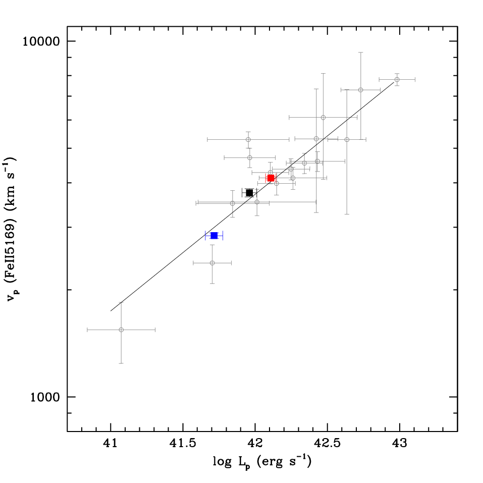
In this paper we take advantage of the homogeneous analysis of the three type II-P SNe (SNe 2012ec, 2012aw and 2012A) to perform a detailed comparison of the available calibrations of SCM and assess the robustness of the method. More specifically, for the comparison we adopt the -band calibrations of SCM, namely: eq. of Hamuy & Pinto (2002); eq. of Nugent et al. (2006); eq. of Poznanski et al. (2009); eq. 2 of D’Andrea et al. (2010)66 6 In passing, we note that the Poznanski et al. (2010) recalibration of this work led to a Hubble diagram with a scatter of only ; and eq. of Olivares et al. (2010). Our estimated distances to the three SNe are compared with a homogeneous set of distances, based on primary (Cepheids, Tip of the Red Giant Branch, or TRGB) and secondary distance indicators (Tully-Fisher, Surface Brightness Fluctuations or SBF), available in the Extragalactic Distance Database (Tully et al., 2009). In Table 11 we report, for each SN, the distance estimated with the above calibrations. Moreover, we show the difference between the SCM distance and the estimates from the primary (when available) and secondary distance indicators. Finally, for each calibration, we report the mean difference and dispersion of the SCM distances with the estimates based on the primary and secondary distance indicators.
| Calibration | SN | SCM | Primary | Secondary | SCM Primary | SCM - Secondary | Mean residual |
|---|---|---|---|---|---|---|---|
| (mag) | (mag) | (mag) | (mag) | (mag) | (mag) | ||
| SN 2012ec | |||||||
| HP2002 | SN 2012aw | ||||||
| SN 2012A | |||||||
| SN 2012ec | |||||||
| Nugent06 | SN 2012aw | ||||||
| SN 2012A | |||||||
| SN 2012ec | |||||||
| Poznanski09 | SN 2012aw | ||||||
| SN 2012A | |||||||
| SN 2012ec | |||||||
| Olivares10 | SN 2012aw | ||||||
| SN 2012A | |||||||
| SN 2012ec | |||||||
| D’Andrea10 | SN 2012aw | ||||||
| SN 2012A |
Quoted errors for the SCM distances are the standard deviations of the individual calibrations. The value of the distance from the primary indicators of SN 2012aw is the average from the Cepheids (Freedman et al., 2001) and the TRGB (Rizzi et al., 2007) estimates. Finally, the “mean residual” column shows the average of the SCM Secondary values, where the error is the standard deviation.
Table 11 may suggest that the Hamuy & Pinto (2002) calibration gives more homogenous results with respect to other calibrations. However, it must be noted that our test is based on only three SNe and that all the calibrations are consistent within the errors. We note that the Hamuy & Pinto (2002) calibration was derived assuming a value of km s-1 Mpc-1, significantly lower than the estimate of km s-1 Mpc-1 of Riess et al. (2011), but in agreement with km s-1 Mpc-1 given by Tammann & Reindl (2013). The large scatter in the Olivares et al. (2010) calibration could be due to the difficulty in estimating the reference phase, when a well sampled light curve covering the end of the plateau, is not available. All these calibrations rely on moderately distant SNe, embedded in the Hubble flow or for which SBF distances are available. However, these distances could still be affected by systematics not completely understood. For these reasons a new calibration of the SCM, based on nearby type II-P SNe for which primary (Cepheids and TRGB) and homogenous secondary indicators (TRGB) distances are available, would be of great interest. Moreover, for these SNe the metallicity effects suggested by Kasen & Woosley (2009) could also be investigated. The average of the five individual estimates of the distances for SN 2012ec gives a distance modulus of mag, which we adopt as our final SCM-based distance. This value is in excellent agreement with the Tully-Fisher distance of , adopted for our analysis.
9 Conclusions
We have presented the results of the Large Program “Supernova Variety and Nuclesosynthesis Yelds” and PESSTO photometric and spectroscopic monitoring campaign of SN 2012ec. This is one of the most intensively observed and well investigated Type II-P SNe to date. The optical and spectrocopic monitoring during the photospheric phase lasted for days and allowed us to determine the evolution of the pseudo-bolometric luminosity, the expansion velocity and the photospheric temperature and mass.
These parameters, analysed in conjunctions with hydrodynamical models, allowed us to estimate the explosion parameters such as the explosion energy, the envelope mass and the pre-SN radius.
Correcting the data for reddening ( mag) and distance modulus () we estimated the luminosity to be , at the plateau and evaluated the mass to be .
The spectra of SN 2012ec were dominated by Balmer lines in the early epochs and after 20 days the iron-group elements started to appear and become more prominent with time. The NIR spectra were dominated by Paschen lines and, starting from 68 days, it is possible to identify He I, Ca I and . A black body fit to the continuum gives temperatures of K in the early epoches decreasing to K at 50 days and K in the last epochs.
From the spectroscopic dataset we estimate an initial velocity of for the line and for . The velocity decreases to by 50 days. At days the iron-group elements appear, for which we measure a velocity of (for Fe II). The behaviour of SN 2012ec is similar to that seen in other II-P SNe, such as SN 1999em (Elmhamdi et al., 2003) and SN 2004et (Maguire et al., 2010).
We estimate the physical parameters of SN 2012ec through the hydrodynamical modeling described in Sect. 6. The fit suggests an ejected mass of , a pre-SN radius of , an explosion energy of and an ejected . The progenitor mass is in agreement with independent estimate of Maund et al. (2013) obtained by analyzing pre-explosion images and of Jerkstrand et al. (2014), submitted, obtained from modeling of the spectra in the nebular phase. Previously reported ejecta masses estimated from hydrodynamical modelling are generally too large compared to the initial mass estimated from direct detections of the progenitor on pre-explosion images (Utrobin & Chugai, 2008; Maguire et al., 2010). In order to investigate this discrepancy, we performed an homogeneous comparison between three type II-P SNe, estimating the mass of the progenitor with two different approaches. The methods and the codes used for the three objects in both cases are the same, to facilitate a reliable comparison. We analyze the bright SN 2012aw (Dall’Ora et al., 2014), the low-luminosity SN 2012A (Tomasella et al., 2013) and SN 2012ec. Several observational and derived parameters have been compared for these three objects. SN 2012aw ( mag, at plateau) is brighter then SN 2012ec ( mag), while SN 2012A is fainter ( mag). A comparison between the bolometric light curves shows that SN 2012ec has an intermediate luminosity between the high luminosity SN 2012aw and the fainter SN 2012A. The nickel mass synthetized by these SNe is , and . A spectroscopic comparison shows a similar time evolution at all epochs. The velocities of , and Fe II of SN 2012ec, place it in the middle of the higher velocities from SN 2012aw and the slowest SN 2012A at all times. The temperatures estimated are comparable for the three objects within the first 20 days, rather SN 2012ec tend to be similar to SN 2012A and they both are hotter than SN 2012aw. SN 2012aw has a more energetic explosion ( foe) than SN 2012ec and SN 2012A ( foe), but SN 2012ec is also more energetic than SN 2012A. We finally compared the results of the direct detection of the progenitors of these three SNe with the masses estimated from the hydrodynamical modelling. The progenitor mass estimated for SN 2012aw from the pre-explosion images () and from the hydrodynamical modeling () show that the two methods are not in good agreement and that SN 2012aw has a more massive progenitor then SN 2012ec, the last one having comparable ejecta mass with SN 2012A (, ). The estimated initial radius of SN 2012aw ( cm) indicate a larger progenitor then for SN 2012ec and SN 2012A ( cm). The estimates of the initial radius from the hydrodynamical modelling for the three objects is lower than those from the pre-explosion images and seem to be too low for a RSG progenitor. This homogeneous analysis finds a substantial match, within the errors, of the mass of the progenitor obtained with the two methods, mitigating the discrepancy which was pointed out in previous works (Maguire et al., 2010). SN 2012ec, SN 2012aw and SN 2012A also follow the relation obtained by Hamuy & Pinto 2002. This fact, coupled with their high luminosity at UV wavelengths, make Type II-P SNe interesting probes observable with the next generation of telescopes up to high z.
10 Acknowledgements
We warmly thank our referee, Dovi Poznanski, for his helpful comments, which significantly improved the content and the readability of our manuscript.
We thank E. Cappellaro for the useful discussions.
C.B. thanks the IRAP PhD program for the financial support. The research of JRM is supported through a Royal Society Research Fellowship. A.G.-Y. is supported by an EU/FP7-ERC grant no [307260], ”The Quantum Universe” I-Core program by the Israeli Committee for planning and budgeting and the ISF, GIF, Minerva, ISF and Weizmann-UK grants, and the Kimmel award. G.P. acknowledges partial support by proyecto interno UNAB DI-303-13/R. GP and MH acknowledge support provided by the Millennium Institute of Astrophysics (MAS) through grant IC120009 of the Programa Iniciativa Cientifica Milenio del Ministerio de Economia, Fomento y Turismo de Chile”. M.D.V., M.L.P., S.B., A.P., L.T. and M.T. are partially supported by the PRIN-INAF 2011 with the project “Transient Universe: from ESO Large to PESSTO”. This work was partly supported by the European Union FP7 programme through ERC grant number 320360.
This work is based (in part) on observations collected at the European Organisation for Astronomical Research in the Southern Hemisphere, Chile as part of PESSTO, (the Public ESO Spectroscopic Survey for Transient Objects Survey) ESO program 188.D-3003, 191.D-0935. The research leading to these results has received funding from the European Research Council under the European Union’s Seventh Framework Programme (FP7/2007-2013)/ERC Grant agreement no [291222] (PI : S. J. Smartt) and STFC grants ST/I001123/1 and ST/L000709/1.
The early SN 2012ec data have been collected via the ESO-NTT Large Program “Supernova Variety and Nuclesosynthesis Yelds” (184.D-1140), an European supernova collaboration led by Stefano Benetti (http://sngroup.oapd.inaf.it/esolarge.html). This paper is partially based on observations collected at Copernico telescope (Asiago, Italy) of the INAF - Osservatorio Astronomico di Padova; at the Galileo 1.22m Telescope operated by Department of Physics and Astronomy of the University of Padova at Asiago; at the 2.56m Nordic Optical Telescope operated by The Nordic Optical Telescope Scientific Association (NOTSA); at the 4.3m William Herschel Telescope operated by the Isaac Newton Group of Telescopes; on observations obtained through the CNTAC proposal CN2012B-73 and on observations made with the Liverpool Telescope (programme OL12B) operated on the island of La Palma by Liverpool John Moores University in the Spanish Observatorio del Roque de los Muchachos of the Instituto de Astrofisica de Canarias with financial support from the UK Science and Technology Facilities Council.
References
- Arcavi et al. (2012) Arcavi I., Gal-Yam A., Cenko S.B. et al., 2012, APJ, 756L, 30A
- Arnett Fu (1989) Arnett W.D. Fu A. 1989, APJ, 340, 396
- Barbon et al. (1979) Barbon R., Ciatti F., & Rosino L., 1979, A&A, 72, 287
- Baron et al. (2004) Baron E., Nugent P.E., Branch D. et al., 2004, APJ, 616, L91
- Bayless et al. (2013) Bayless A.J., Pritchard T.A., Roming P.J., et al., 2013, APJ, 764L, 13B
- Bersten et al. (2012) Bersten M.C., Benvenuto O., Nomoto K. et al., 2012, APJ, 757, 31B
- Blinnikov et al. (2000) Blinnikov S., Lundqvist P., Bartunov O., et al. 2000, APJ, 532, 1132B
- Botticella et al. (2012) Botticella M.T., Trundle C., Pastorello A. et al., 2010, ApJ, 717L, 52B
- Bose et al. (2013) Bose S., Kumar B., Sutaria F. et al., 2013, MNRAS, 433, 1871B
- Botticella et al. (2012) Botticella M.T., Smartt S.J., Kennicutt R.C. et al., 2012, AA, 537A, 132B
- Bouchet et al. (1991) Bouchet P., Danziger I.J. Lucy L.B. 1991, AJ, 102, 1135
- Cappellaro et al. (1999) Cappellaro E., Evans R. Turatto M. 1999, A&A, 351, 459
- Cardelli et al. (1989) Cardelli J.A., Clayton G.C. Mathis J.S. 1989, APJ, 345, 245
- Carpenter (2001) Carpenter J.M., 2001, AJ, 121, 2851
- Clocchiatti et al. (1996) Clocchiatti A., Benetti S., Wheeler J.C., et al. 1996, AJ, 111, 1286C
- Coppola et al. (2011) Coppola G., Dall’Ora M., Ripepi V., et al. 2011, MNRAS, 416, 1056C
- Childress et al. (2012) Childress M., Scalzo R., Yuan F., Schimdt B., 2012, Central Bureau Electronic Telegrams, 3201, 2
- Chugai Utrobin (2000) Chugai N.N., Utrobin V.P., 2000, AA, 354, 557C
- D’Andrea et al. (2010) D’Andrea C.B., Sako M., Dilday B., et al. 2010, APJ, 708, 661D
- Dalhen et al. (2012) Dalhen T., Strolger L.G., Riess A.G., et al. 2012, APJ, 757, 70D
- Dall’Ora et al. (2014) Dall’Ora M., Botticella M.T., Pumo L., et al. 2014, APJ, 787, 139
- Dessart Hillier (2005) Dessart L., Hillier D.J., 2005, AA, 439, 671
- Eastman, Schmidt Kirshner (1996) Eastman R.G., Schmidt B.P. Kirshner R., 1996, ApJ, 466, 911E
- Eldridge Tout (2004) Eldridge J.J. Tout C.A., 2004, MNRAS, 353, 87E
- Elmhamdi et al. (2003) Elmhamdi A., Danziger I.J., Chugai N. et al., 2003, MNRAS, 338, 939E
- Elmhamdi, Chugai Danzinger (2003) Elmhamdi A.,Chugai N., Danziger I.J., 2003, AA, 404, 1077E
- Faran et al. (2014) Faran T., Poznanski D., Filippenko A.V., et al., 2014, MNRAS, 442, 844F
- Filippenko (1997) Filippenko A.V., 1997, ARAA, 35, 309
- Fraser et al. (2012) Fraser M., Maund J.R., Smartt S.J., et al., 2012, APJ, 759L, 13F
- Freedman et al. (2001) Freedman W.L., Madore B.F., Gibson B.K., et al., 2001, APJ, 553, 47F
- Gilmozzi et al. (1987) Gilmozzi R., Cassatella A., Clavel J., et al., 1987, Nature, 328, 318G
- Grassberg et al. (1971) Grassberg E.K., Imshennik V.S., Nadyozhin D.K., 1971, ApSS, 10, 28G
- Gustafsson et al. (2008) Gustafsson B., Edvardsson B., Eriksson K., 2008, AA, 486, 951G
- Hamuy et al. (2001) Hamuy M. et al., 2001, APJ, 566, L63
- Hamuy Pinto (2002) Hamuy M. Pinto P., 2002, APJ, 558, 615
- Harutyunyan et al. (2008) Harutyunyan A., Pfahler P., Pastorello A., 2008, AA, 488, 383H
- Heger et al. (2003) Heger A., Fryer C.L., Woosley S.E., Langer N., Hartmann D.H., 2003, APJ, 591, 288
- Hook (2013) Hook I.M., 2013, Royal Society of London Philosophical Transactions Series A, 371, 20282
- Hopkins et al. (2006) Hopkins P.F., Somerville R.S., Hernquist L., et al., 2006, APJ, 652, 864H
- Iben Renzini (1983) Iben I. Renzini A., 1983, ARAA, 21, 271
- Inserra et al. (2011) Inserra C., Turatto M., Pastorello A. et al, 2011, MNRAS, 417, 261I
- Inserra et al. (2012) Inserra C., Turatto M., Pastorello A. et al, 2012, MNRAS, 422, 1122
- Jerkstrand et al. (2012) Jerkstrand A., Fransson C., Maguire K. et al, 2012, A&A, 546A, 28J
- Jerkstrand et al. (2014) Jerkstrand A., Smartt S.J., Fraser M. et al, 2014, MNRAS, 439, 3694J
- Jerkstrand et al. (2014) Jerkstrand, A., Smartt, S. J., Sollerman, J., et al. 2014, arXiv:1410.8394
- Kasen Woosley (2009) Kasen D. Woosley S.E., 2009, APJ, 703, 2205
- King et al. (1998) King J.Y., Modjaz M., Shefler T. et al, 1998, IAUC, 6992, 1
- Kirshner Kwan (1974) Kirshner R.P. Kwan J., 1974, APJ, 193, 27K
- Kirshner et al. (1987) Kirshner R.P., Sonneborn G., Crenshaw D.M., et al., 1987, APJ, 320, 602K
- Kleiser et al. (2011) Kleiser, I. K. W., Poznanski, D., Kasen, D., et al. 2011, MNRAS, 415, 372
- Kochanek et al. (2012) Kochanek C.S., Khan R. Dai X., 2012, APJ, 759, 20K
- Kowal (1968) Kowal C.T., 1968, AJ, 73, 1021K
- Landolt (1992) Landolt A.U., 1992, AJ, 104, 340L
- Leonard et al. (2002) Leonard D.C. et al., 2002, PASP, 114, 35L
- Li et al. (2009) Li W., Cenko S.B. Filippenko A.V., 2009, Central Bureau Electronic Telegrams, 1656, 1
- Li et al. (2011) Li W., Leaman J., Chornork R., et al., 2011, MNRAS, 412, 1441
- Litvinova Nadezhin (1983) Litvinova I. Yu., Nadezhin D.K., 1983, ApSS, 89, 89L
- Litvinova Nadezhin (1985) Litvinova I. Yu., Nadezhin D.K., 1985, Pis’ma Astron. Zh., 11, 351
- Maguire et al. (2010) Maguire K., et al. 2010, MNRAS, 404, 981
- Massey et al. (2000) Massey P., Waterhouse E. DeGioia-Eastwood K., 2000, AJ, 119, 2214
- Massey et al. (2001) Massey P., DeGioia-Eastwood K. Waterhouse E. 2001, AJ, 121, 1050
- Maund et al. (2013) Maund J.R., Fraser M., Smartt S.J., et al. 2013, MNRAS, 413L, 102M
- Mitchell et al. (2002) Mitchell R.C., Baron E., Branch D., et al. 2002, ApJ, 574, 293M
- Moiseev (2000) Moiseev A.V., 2000, A&A, 363, 843M
- Monard (2012) Monard L.A.G., 2012, Central Bureau Electronic Telegrams, 3201, 1
- Mould et al. (2000) Mould J.R., Huchra J.P., Freedman W.L., et al. 2000, APJ, 529, 786M
- Nakano et al. (1996) Nakano S., Aoki M., Kushida Y. et al, 1996, IAUC, 6442, 1
- Nakano (2006) Nakano S., 2006, CBET, 470, 1N
- Nugent et al. (2006) Nugent P., Sullivan M., Ellis R., et al. 2006, APJ, 645, 841
- Olivares et al. (2010) Olivares E.F., Hamuy M., Pignata G., et al. 2010, APJ, 715, 833
- Pastorello et al. (2004) Pastorello A., Zampieri L., Turatto M., et al. 2004, MNRAS, 347, 74P
- Pastorello et al. (2009) Pastorello A., Valenti S., Zampieri L., et al. 2009, MNRAS, 394, 2266P
- Pastorello et al. (2009) Pastorello A., Crockett R.M., Martin R., et al. 2009, AA, 500, 1013P
- Pastorello et al. (2012) Pastorello A., Pumo M.L., Navasardyan H., et al. 2012, AA, 537A, 141P
- Perlmutter et al. (1999) Perlmutter S., Aldering G., Goldhaber G., et al. 1999, APJ, 517, 565P
- Poznanski (2013) Poznanski, D. 2013, MNRAS, 436, 3224
- Poznanski et al. (2009) Poznanski D., Butler N., Filippenko A.V., et al. 2009, APJ, 694, 1067
- Poznanski et al. (2010) Poznanski, D., Nugent, P. E., & Filippenko, A. V. 2010, APJ, 721, 956
- Poznanski et al. (2012) Poznanski D., Prochaska J.X., Bloom J.S. 2012, MNRAS, 426, 1465P
- Pumo et al. (2010) Pumo M.L., Zampieri L. Turatto M., 2010, MSAIS, 14, 123
- Pumo Zampieri (2011) Pumo M.L. Zampieri L., 2011, APJ, 741, 41
- Quimby et al. (2007) Quimby R.M., Wheeler J.G., et al. 2007, APJ, 666, 1093
- Ramya et al. (2007) Ramya S., Sahu D.K. Prabhu T.P., et al. 2007, MNRAS, 381, 511
- Riess et al. (1998) Riess A.g., Filippenko A.V., Challis P., et al. 1998, AJ, 116, 1009R
- Riess et al. (2011) Riess A.G., Macri L., Casertano S., et al. 2011, APJ, 730, 119R
- Rizzi et al. (2007) Rizzi L., Tully R.B., Makarov D., et al. 2007, APJ, 661, 815R
- Roy et al. (2014) Roy R., Sutaria F., Bose S., et al. 2007, IAUS, 296, 116R
- Rubin et al. (2013) Rubin D., Knop R.A., Rykoff E., et al. 2013, ApJ, 763, 35R
- Schlafly Finkbeiner (2011) Schlafly E.F. Finkbeiner D.P., 2011, APJ, 737, 103
- Schlegel et al. (1998) Schlegel, D. J., Finkbeiner, D. P., & Davis, M. 1998, APJ, 500, 525
- Schmidt et al. (1994) Schmidt B.P., Kirshner R.P., Eastman R.G., 1994, APJ, 432, 42S
- Schmidt et al. (1998) Schmidt B.P., Suntzeff N.B., Phillips M.M., 1998, APJ, 507, 46S
- Skrutskie et al. (2006) Skrutskie M.F., Cutri R.M., Stiening R., et al. 2006, AJ, 131, 1163
- Smartt (2009) Smartt S.J., 2009, ARAA, 47, 63
- Smartt et al. (2009) Smartt S.J., Eldridge J.J., Crockett R.M., 2009, MNRAS, 395, 1409S
- Smartt et al. (2014) Smartt, S. J., Valenti, S., Fraser, M., et al. 2014, arXiv:1411.0299
- Smith et al. (2002) Smith J.A., Tucker D.L., Kent S., 2002, AJ, 123, 2121S
- Spiro et al. (2014) Spiro S, Pastorello A., Pumo M.L., 2014, MNRAS, 439, 2873S
- Stetson (1987) Stetson P.B., 1987, PASP, 99, 191S
- Suntzeff et al. (1988) Suntzeff N.B., Hamuy M., Martin G. et al., 1988, AJ, 96, 1864S
- Tammann Reindl (2013) Tammann G.A. Reindl B., 2013, AA, 549A, 136T
- Tomasella et al. (2013) Tomasella L., Cappellaro E., Fraser M., et al. 2013, MNRAS, 434, 1636T
- Tully et al. (2009) Tully R., Rizzi L., Shaya E.J., et al. 2009, AJ, 138, 323T
- Turatto et al. (2003) Turatto M., Benetti S., Cappellaro E. 2003, in From Twilight to Highlight: The Physics of Supernovae, ed. W. Hillebrandt B. Leibundgunt, 200
- Utrobin (1993) Utrobin V.P., 1993, AA, 281L, 89U
- Utrobin (2007) Utrobin V.P., 2007, AA, 461, 233U
- Utrobin et al. (2007) Utrobin V.P., Chugai N.N., Pastorello A. 2007, AA, 475, 973U
- Utrobin Chugai (2008) Utrobin V.P. Chugai N.N., 2008, AA, 491, 507U
- Utrobin Chugai (2009) Utrobin V.P. Chugai N.N., 2009, AA, 506, 829U
- Valenti et al. (2011) Valenti S., Fraser M., Benetti S., et al. 2011, MNRAS, 416, 3138
- Van Dyk et al. (2012) Van Dyk S.D., Cenko S.B., Poznanski D., et al. 2012, APJ, 756, 131V
- Walmswell Eldridge (2012) Walmswell J.J. Eldridge J.J., 2012, MNRAS, 419, 2054
- Weaver Woosley (1980) Weaver T.A., Woosley S.E., 1980, AIPC, 63, 15W
- Woosley et al. (2002) Woosley S.E., Heger A., Weaver T.A. 2002, Rev. Mod. Phys., 74, 1015
- Yaron Gal-Yam (2012) Yaron O., Gal-Yam A. 2012, PASP, 124, 668Y
- Zampieri et al. (1998) Zampieri L., Shapiro S.L., Colpi M., et al. 1998, ApJ, 502L, 149Z
- Zampieri et al. (2003) Zampieri L., Pastorello A., Turatto M., et al. 2003, MNRAS, 338, 711
- Zampieri (2005) Zampieri L., 2005, ASPC, 342, 358Z
- Zampieri (2007) Zampieri L., 2007, AIPC, 924, 358Z