Modelling overdispersion heterogeneity
in differential expression analysis using mixtures
Abstract
Next-generation sequencing technologies now constitute a method of choice
to measure gene expression. Data to analyze are read counts,
commonly modeled using Negative Binomial distributions. A relevant
issue associated with this probabilistic framework is the reliable
estimation of the overdispersion parameter, reinforced by the
limited number of replicates generally observable for each gene. Many
strategies have been proposed to estimate this parameter, but when
differential analysis is the purpose, they often result in procedures
based on plug-in estimates, and we show here that this discrepancy
between the estimation framework and the testing framework can lead to
uncontrolled type-I errors. Instead we propose a mixture
model that allows each gene to share information with other genes that exhibit similar variability. Three consistent statistical tests are
developed for differential expression analysis. We show that the proposed method improves the
sensitivity of detecting differentially expressed genes with respect to the common procedures, since it is the best one in reaching the nominal value for the
first-type error, while keeping elevate power. The method is finally illustrated on prostate cancer RNA-seq data.
KEYWORDS: Hypothesis testing; Mixture models; RNA-seq data.
1 Introduction
Massive parallel sequencing has deeply changed our understanding of gene expression thanks to a higher resolution (Soon et al., 2013; Wang et al., 2009). From the analysis point of view, NGS experiments provide discrete read counts assigned to target genome regions measuring the expression level or the abundance of the target transcript. When the purpose of the assay is to perform differential analysis, that is comparing the counts of a given regions between conditions, the statistical task is then to provide an appropriate model to account for biological and technical variations, as well as a testing framework to test the hypothesis of no difference. Here we deal with the case where regions of interest are given a priori, contrarily to analysis where the regions themselves have to be discovered (Frazee et al., 2014). Generalized linear models based on count distributions now constitute a consensus framework for the analysis, with the original Poisson distribution (Marioni et al., 2008; Wang et al., 2010) being replaced by the Negative Binomial model (Robinson and Smyth, 2008; Anders and Huber, 2010; Robinson et al., 2010). Indeed, the simplest choice of the Poisson distribution was rapidly identified as the cause of uncontrolled first-type errors, due to a poor adjustment to the larger observed variability compared with the equal mean-variance specification of the Poisson model (see, for a discussion, Anders and Huber (2010)). Since then, the correct modeling and estimation of this observed overdispersion has been a key issue in differential analysis.
Taking perspective from our past experience in micro-array analysis, the proper modeling of the dispersion parameter has long been a subject of debate in differential analysis, with a difficult trade-off between a common variance for every genes and gene-specific variances. Given the limited number of replicates, the first strategy provides robust estimates, but the testing procedure lacks of power and the model is not realistic, whereas the second is more sensitive at the price of increased first-type errors. Actually, the debate is still ongoing with the Negative Binomial framework, but the problem is much more difficult to solve due to this complex (and unknown) mean-variance relationship.
Several contributions have been proposed to find a trade-off between the common overdispersion and the gene-specific overdispersion frameworks. Robinson and Smyth (2008) addressed the problem in a multi-step procedure called edgeR. They first proposed to estimate a common dispersion parameter for all genes expressed as a quadratic combination of the mean, and then, by making use of a weighted likelihood procedure, they provide an estimation of each dispersion parameter as a weighted combination of the common and of the individual ones, assuming empirical weights. Then an approximation is introduced in order to develop an exact test. Anders and Huber (2010) proposed to use a mean-dependent local regression to smooth the gene-specific dispersion estimates, related to the idea that genes that share a similar mean expression level have also a similar variance, and therefore they can contribute to the estimation of the respective parameters. The method is implemented in the DESeq R package. Wu et al. (2013) introduced an empirical Bayes shrinkage approach choosing a log-normal prior distribution on the dispersion parameters and therefore imposing a negative binomial likelihood. Then the estimations are plugged-in the Wald statistic to perform the statistical test. The method is implemented in the DSS R library. In the Hardcastle and Kelly (2010) proposal, the dispersion is iteratively estimated using the quasi-likelihood approach. A comparison of all these existing approach has been illustrated in Yu et al. (2013), where a new strategy based on the method of the moments is employed in order to get reliable dispersion parameters estimation.
Despite the rapidly increasing diffusion of these statistical procedures, also thanks to the availability of the well documented Bioconductor packages such as edgeR, DESeq and DSS, the estimation of the dispersion in NGS data remains a crucial and tricky issue because of the limited number of available observations for each gene. Moreover, less attention has been focused on the consistency between the estimation and the testing frameworks. Indeed, an important drawback of using plug-in estimators is that the expected variations of the test statistics are no longer controlled under the null hypothesis, which may result in an un-controlled level of the test. We will illustrate this point in a simulation study, by showing that most proposed methods do not reach the nominal level of the test, whereas it is precisely what is expected to be controlled when performing standard hypothesis testing.
Our contribution is to explore and discuss a mixture model approach (McLachlan and Peel, 2000; Fraley and Raftery, 2002) based on the idea of sharing information among genes that exhibit similar dispersion. More specifically, mixtures of negative binomial distributions are investigated as a way to get more accurate estimation for the dispersion parameter of each gene, exploiting also the information provided by the others. Such an approach has already be considered in the same context for the differential analysis of microarray data (Delmar et al., 2005). A consistent statistical testing procedure is then developed within the unified model based clustering framework. The proposed method improves the sensitivity of detecting differentially expressed genes with small replicates, and we show that our method controls the nominal level of the test by simulation.
The novel method will be described in Section 2. We will derive three statistical tests and describe the procedure for performing the differential analysis in Section 3. We will show through a large simulation study in Section 4 that the proposed statistical test procedure outperforms the mostly used strategies in the literature, because it is the best one in reaching the nominal value for the first-type error, while keeping elevate power, thus indicating its inferential reliability. The method will be applied on prostate cancer data in Section 5. A final discussion is presented in Section 6.
2 The proposed method
2.1 The data problem
Suppose we observe the read counts of genes in biological conditions. For each condition, assume that replicates are available, with . Without loss of generality, here we consider . We denote the random variable that expresses the read counts, say , mapped to gene (=), in condition , in sample (= ). Let be the random vector of length denoting the expression profile of a gene. Let be the observed value. Analogously, , is the vector of length containing the observed gene profile under condition . Let us consider the Negative Binomial distribution (NB), with parameters , , expectation and variance (see, for instance, Hilbe (2011)), so that is the location parameter and is the dispersion parameter. For a random variable we have
| (1) |
By assuming that the read counts can be described by the distribution in (1), ideally we would fit the model
for each gene and then we would test the null hypothesis . In most experiments, replicates are too few to accurately estimate both parameters for each gene (usually less than 20). To overcome the limitedness of the available observations, we propose to aggregate information of genes sharing similar variability thought a mixture model that jointly consider all the genes. The proposal constitute a trade-off between the gene specific variance model and the one with common dispersion parameter.
2.2 The model
An interesting characteristic of the NB parametrization in (1) is that it can be derived from a Poisson-Gamma mixed distribution. More precisely, if the random variable follows the Gamma distribution with unit mean
and the random variable conditional on follows the Poisson distribution
then unconditionally is distributed according to the NB, . This means that the parameter of the Poisson component rules the expectation of the negative binomial distribution, and the parameter of the gamma component controls the heterogeneity, thus allowing overdispersion.
Instead of fitting different NB models, we consider a unified mixture model approach for all the genes. In order to develop it, notice that the data can be viewed in a multilevel structure, where the first-level units are the replicates (), at the second level we have the conditions () and at the third level there are the genes (). By considering the replicates independent draws within and between conditions we have
| (2) |
We consider a mixture model for the units at the third level of this hierarchical structure. More precisely, we assume that the heterogeneity component contains independent replicates with distribution given by a mixture of gamma components:
| (3) |
It is possible to show that if then follows a mixture of NB distributions:
| (4) |
Proof is given in the Appendix.
In the mixture model (4) the genes are clustered according to their variability only. Conditionally on each group , the density of the generic read count is a negative binomial with gene-wise and condition-wise mean equal to and variance equal to .
2.3 Model estimation
Let be the whole set of model parameters. The log-likelihood of the model is given by
| (5) |
A direct maximization of (5) is not analytically possible, but the maximum likelihood estimates can be derived by the EM algorithm (Dempster et al., 1977). The algorithm alternates between the expectation and the maximization steps until convergence, with the aim of maximizing the conditional expectation of the so-called complete log-likelihood given the observable data. The complete log-likelihood is the joint log-density of the observable data and of the missing data of the model. In the proposed mixture model, the hidden data consists of two sets of latent variables, which are (1) the latent variable deriving by considering the NB distribution as a gamma-poisson mixed process and (2) the latent allocation -vector, , that contains the 1 if the gene belongs to the group and zero otherwise. The complete log-likelihood can be defined as
| (6) | |||||
where , and is the multinomial distribution
In the EM algorithm we maximize the conditional expectation of the complete density given the observable data, using a fixed set of parameters :
| (7) |
which leads to iterating the E and M steps until convergence. The details of the algorithm are described in the Appendix. The EM algorithm has been implemented in R code and a CRAN package will be available soon.
3 Differential analysis
In this section, the procedure to identify the genes () that differentially express under two () different biological conditions is described. This aim can be accomplished in different ways: one could be interested in evaluating the equality between the two population means, or in checking wether their ratio is equal to 1, or wether the log-ratio is zero. The three scenarios can be represented by the following null hypotheses:
- 1.
“Difference”:
- 2.
“Ratio”:
- 3.
“Log Ratio”:
For each case, we can evaluate a test-statistic based on the EM estimates. Since the EM estimators are maximum likelihood estimators, the test-statistics are asymptotically distributed according to the standard Gaussian under the null hypothesis:
- 1.
For the “Difference” test statistic: ,
- 2.
for the “Ratio” test statistic: ,
- 3.
for the “Log Ratio” test statistic: ,
where and are the EM-estimators.
The “Difference” statistical test
For computing the test statistic we need to estimate the variance at the denominator of the test statistics. First of all we notice that since the covariance is zero by the model assumptions. The specific variances are a function of . In particular, and denoting as
| (8) |
The variance can be computed by observing that the replicates , with are independently distributed according to a mixture of NB, so that and for mixture models the general formula for the variance holds
where because the expectation is not component varying; as regards we considered the conditional expectation given the observed data because of the multilevel structure of the data, and therefore
| (9) |
This formula enlightens the effect of the mixture model we propose:
the over-dispersion term is a weighted average of the (estimated)
over-dispersion terms one would get in each
component of the mixture. These terms are weighted according to the
posterior probability for observation to belong to each component
: .
The “Ratio” statistical test
As for the computation of we can use Delta method (van der Vaart (2000); Cox (1990)), and by simple computations we get:
All the needed quantities can be computed easily. With regards to we can use the EM estimates for because they are correct. For the variances we make use of the procedure described above.
The “Log Ratio” statistical test
The variance at the denominator of the statistical test can be decomposed as . Now we observe that . According to the Delta method and in our case the Delta approximation for the variance is .
4 Simulation study
The performance of the proposed strategy is evaluated by a large simulation study comprising several data generating processes with the double aim of: (a) assessing the capability of the proposed mixture model to estimate the variances with a specified number of components, and (b) evaluating the accuracy of the three statistical test procedures in terms of power and first-type error. In particular, in a set of multiple tests in the absence of correction, a reliable statistical test should reach the nominal significance level as increases. We compare the three proposed statistical tests with the procedures of Robinson et al. (2010), Anders and Huber (2010) and Wu et al. (2013) and implemented in the packages edgeR, DESeq and DSS respectively.
4.1 Simulation A
In the first simulation study, we evaluated the capability of the proposed mixture model to estimate the variances of the genes as the number of components, , increases. Indeed, our purpose is to account for heterogeneity among the overdispersion parameters and we do not necessarily believe that groups of differently overdispersed genes do exist. In the limit, the number of overdispersion parameters could be equal to the number of genes, and we want to test if our strategy will adapt to such a situation. We also computed some conventional information criteria in order to select the optimal number of components.
A set of datasets with genes, conditions and replicates have been simulated. The of the genes (= 100 genes) are supposed to be differentially expressed (), while the remaining genes (= 200 genes) have been generated with . For the 100 differentially expressed genes we generated and where is randomly drawn from a ; for the 200 non-differentially expressed genes we considered . For all the genes the dispersion parameters have been randomly drawn from a . All the values for the parameters have been chosen to be consistent with the empirical situation.
On each dataset we fitted the proposed mixture model for ranging from 1 to 6. Figure 1 shows the average of the relative distances in absolute values across the 100 datasets between the estimated variances by (8) and the true ones as varies. In computing the (8), we applied the correction factor in order to obtain the corresponding correct estimator. The dashed lines denote the standard error bands computed as mean standard error. From the graph, we could say that from components the gain of fitting more complex mixture models becomes irrelevant. In other terms, it seems that and components well describe the variability of the genes.
This insight is also confirmed by the information criteria. More specifically, we have considered the Akaike’s Information Criterion (Akaike (1974)), , where is the total number of required parameters and the more conservative Bayesian Information Criterion (Schwarz et al. (1978)), . In addition, we have also computed the so-called Integrated Classification Likelihood criterion (Biernacki et al. (2000)) that combines the BIC penalty term with the entropy of the posterior classification. As a result, ICL-BIC is characterized by a heavier penalty term and it tends to favour simpler model against mixture models with more components.
| AIC | BIC | ICL-BIC | |
|---|---|---|---|
| 1 | 0 | 0 | 0 |
| 2 | 0 | 2 | 76 |
| 3 | 76 | 86 | 24 |
| 4 | 6 | 4 | 0 |
| 5 | 6 | 4 | 0 |
| 6 | 12 | 4 | 0 |
In Table 1 the number of times each criterion suggests a specific number of components is shown. These results recommend that mixture components are enough to give a good description of the data. The capability of estimating the dispersions and therefore the variances for each method has been checked through the computation of the average relative errors between the true variances and the ones estimated by each analyzed strategies. In Figure 1 the relative distances between the estimated and true variances as varies and the correspondent boxplots are presented. It is clear from this graph that the proposed method greatly improves the accuracy of the variance estimation.

, 
4.2 Simulation B
In this simulation study we considered the same simulation design presented before with a varying number of replicates . For each case we generated datasets. Then the mixture model with components has been estimated on the data and the three proposed test statistics have been computed. The adequateness of the statistical procedures can be evaluated by observing the approximation towards the nominal significance level under the null hypothesis as the number of replicates increases. For each of the 200 not-differentially expressed genes, we have computed the empirical first-type errors across the 1000 datasets for the three statistics. For comparative purposes, we have also computed the null p-values provided by DESeq, edgeR and DSS on the same data. Figure 2 contains the box-plots of the empirical first-type errors obtained by the “Difference” test statistic and of the other considered approaches as the number of replicates varies and for the different levels of the test (0.05, 0.01 and 0.001).
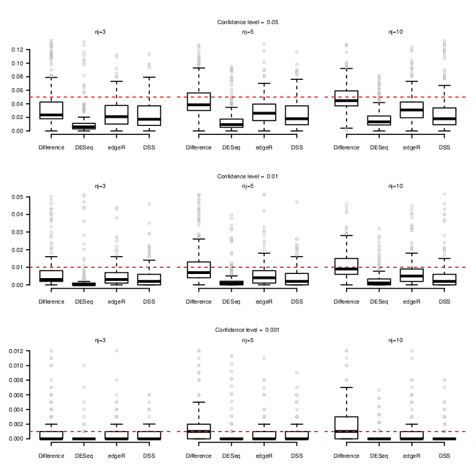
The three statistical tests fast converge to the nominal level as the number of the replicates increases, while the DESeq, edgeR and DSS based tests are always under the nominal level. It is clear from these graphs that the proposed test statistics are the only ones that actually reach the nominal value for the first-type error. The distribution of the first-type errors that have been obtained from the estimations provided by edgeR and DSS crosses the nominal values only with the upper whisker, and DESeq distribution does not cross the nominal value at all.
The capability of controlling the first-type error can be checked also looking at the empirical cumulative distribution function (ECDF) of the null p-values; the more their distribution is close to the diagonal, the more they can be considered as actually uniformly distributed, as requested by the probability integral transform theorem. In Figure 3 the ECDFs for the null p-values obtained through the proposed test statistics, DESeq, edgeR and DSS as varies are shown. It is clear that the proposed test statistics behave better than the others already in correspondence of , then the correspondent ECDFs become closers and closers to the diagonal as the number of replicates increases and for the ECDF for the null p-values of the proposed procedures even overlap the diagonal, whereas edgeR, DESeq and DSS reveal curves that lie behind the diagonal for all the three scenarios.

The means and standard errors of the first-type and second-type errors have been reported in Tables 2 and 3. It is important to underline that the distributions of the first- and second-type errors are very skewed especially with regards to DESeq, edgeR and DSS. It is possible to assay that the proposed test procedures (and in particular the “Difference” and the “Log Ratio”), in addition to being able to control the false-positive rates, are good also in containing the false-negative ones.
| Statistic | |||
|---|---|---|---|
| Confidence level= 0.05 | |||
| Difference | 0.0392 (0.0356) | 0.0483 (0.0273) | 0.0505 (0.0213) |
| Ratio | 0.0418 (0.0351) | 0.0501 (0.0267) | 0.0516 (0.0211) |
| Log Ratio | 0.0395 (0.0366) | 0.0485 (0.0278) | 0.0506 (0.0217) |
| DESeq | 0.0143 (0.0242) | 0.0172 (0.0206) | 0.0201 (0.0187) |
| edgeR | 0.0337 (0.0454) | 0.0333 (0.0335) | 0.0346 (0.0229) |
| DSS | 0.0380 (0.0624) | 0.0352 (0.0499) | 0.0293 (0.0318) |
| Confidence level= 0.01 | |||
| Difference | 0.0107 (0.0179) | 0.0121 (0.0134) | 0.0119 (0.0098) |
| Ratio | 0.0135 (0.0197) | 0.0146 (0.0142) | 0.0131 (0.0104) |
| Log Ratio | 0.0110 (0.0190) | 0.0123 (0.0138) | 0.0120 (0.0100) |
| DESeq | 0.0036 (0.0111) | 0.0034 (0.0072) | 0.0037 (0.0061) |
| edgeR | 0.0102 (0.0252) | 0.0085 (0.0155) | 0.0074 (0.0085) |
| DSS | 0.0128 (0.0382) | 0.0102 (0.0260) | 0.0066 (0.0125) |
| Confidence level= 0.001 | |||
| Difference | 0.0031 (0.0086) | 0.0025 (0.0047) | 0.0021 (0.0032) |
| Ratio | 0.0045 (0.0105) | 0.0037 (0.0063) | 0.0026 (0.0039) |
| Log Ratio | 0.0033 (0.0092) | 0.0027 (0.0051) | 0.0021 (0.0034) |
| DESeq | 0.0012 (0.0053) | 0.0007 (0.0023) | 0.0005 (0.0012) |
| edgeR | 0.0032 (0.0126) | 0.0018 (0.0058) | 0.0012 (0.0024) |
| DSS | 0.0048 (0.0211) | 0.0032 (0.0117) | 0.0013 (0.0038) |
| Statistic | |||
|---|---|---|---|
| Confidence level= 0.05 | |||
| Difference | 0.1582 (0.2738) | 0.1002 (0.2267) | 0.0543 (0.1455) |
| Ratio | 0.2112 (0.3259) | 0.1304 (0.2812) | 0.0764 (0.2046) |
| Log Ratio | 0.1569 (0.2726) | 0.0991 (0.2246) | 0.0534 (0.1443) |
| DESeq | 0.1987 (0.3007) | 0.1196 (0.2568) | 0.0642 (0.1809) |
| edgeR | 0.1444 (0.2526) | 0.0945 (0.2197) | 0.0529 (0.1533) |
| DSS | 0.1354 (0.2449) | 0.0892 (0.2109) | 0.0513 (0.1526) |
| Confidence level= 0.01 | |||
| Difference | 0.2341 (0.3289) | 0.1442 (0.2867) | 0.0874 (0.2199) |
| Ratio | 0.3336 (0.3874) | 0.1897 (0.3334) | 0.1146 (0.2775) |
| Log Ratio | 0.2331 (0.3278) | 0.1430 (0.2845) | 0.0856 (0.2167) |
| DESeq | 0.3141 (0.3472) | 0.1755 (0.3102) | 0.0980 (0.2462) |
| edgeR | 0.2268 (0.2997) | 0.1384 (0.2740) | 0.0815 (0.2170) |
| DSS | 0.2159 (0.3014) | 0.1357 (0.2710) | 0.0813 (0.2181) |
| Confidence level= 0.001 | |||
| Difference | 0.3441 (0.3703) | 0.2037 (0.3345) | 0.1228 (0.2834) |
| Ratio | 0.5075 (0.3996) | 0.2889 (0.3847) | 0.1545 (0.3260) |
| Log Ratio | 0.3433 (0.3693) | 0.2026 (0.3333) | 0.1212 (0.2799) |
| DESeq | 0.4873 (0.3635) | 0.2620 (0.3572) | 0.1382 (0.3016) |
| edgeR | 0.3609 (0.3359) | 0.2066 (0.3193) | 0.1166 (0.2753) |
| DSS | 0.3508 (0.3471) | 0.2061 (0.3230) | 0.1176 (0.2758) |
5 Application to Prostate Cancer Data
We have analyzed data on RNA-Seq data on prostate cancer cells collected in two different conditions: a group of patients has been treated with androgens, and the
second one with an inactive compound. The data have been sequenced and analyzed by Li et al. (2008). It is well known that androgen hormones stimulate some genes,
and they also have a positive effect in curing prostate cancer cells. Therefore the connection between these stimulated genes and the survival of these cells is a
largely studied issue.
Seven biological replicates of prostate cancer cells (three for the androgen-treated condition and four for the control-group) for genes have been
sequenced using the Illumina 1G Genome Analyzer. Then they have been mapped to the NCBI36 build of the human genome using Bowtie (allowing up to two mismatches)
and then the number of reads that corresponded to each Ensembl gene (version 53) was counted. The resulting read count table is available from
https://sites.google.com/site/davismcc/useful-documents. For the analysis we have considered the genes with mean count greater than 1, because
they provide sufficient statistical information on the differential analysis. In order to account for the bias introduced by the different lanes of the experiment and the eventual effect the gene length, we preliminarily normalized the data using quantile-based normalization scheme implemented in the R package EDASeq (see, among the others, Risso et al. (2011), Tarazona et al. (2011), Dillies et al. (2013), Bullard et al. (2010)).
5.1 Analysis and Results
The proposed NB mixture model has been fitted on the data with a
number of components ranging from 1 to 6. The BIC and AIC criteria
suggested components. Convergence has been obtained with 50
iterations of the EM-algorithm at the log-likelihood of -384886 (BIC=
1088660, AIC= 835479). Differential expression analysis has been
conducted by computing the three proposed test statistics. For
comparative purposes we have performed differential analysis using the
DESeq, edgeR and DSS methods implemented in
R using the default settings. The estimation of the dispersion
parameters have been obtained with the following R commands:
estimateDispersions for DESeq,
estimateTagwiseDisp for edgeR and estDispersion
for DSS.
All the obtained p-values have been adjusted following the procedure of Benjamini and Hochberg (1995) in order keep under control the total first error in multiple comparison testing. In Table 4 the number of genes declared DE by each method at the confidence levels of 0.05, 0.01 and 0.001 is shown. The different methods detect a proportion of DE genes ranging from about 10 to 25. In order to investigate the degree of accordance between two methods, we measured the proportion between the number of genes declared DE jointly by both methods and the average number of the genes declared DE marginally at a certain confidence level.
| Statistic | |||
|---|---|---|---|
| Difference | 3167 | 2146 | 1360 |
| Ratio | 3538 | 2591 | 1914 |
| Log Ratio | 4254 | 2941 | 2024 |
| DESeq | 2695 | 1828 | 1271 |
| edgeR | 3918 | 2774 | 1886 |
| DSS | 4215 | 2737 | 1737 |
The first panel of Figure 4 shows the pairwise comparison between the proposed “Difference” test statistic and the DESeq, edgeR and DSS methods. The other two pictures of Figure 4 show the same results for the “Ratio” and “Log Ratio” test statistics respectively.

,  ,
,

It is clear from these graphs that the proposed test statistics provide results that are strongly consistent with the ones obtained by edgeR and DSS, with a degree of accordance of about 90 when the “Difference” or the “Log Ratio” is used. The set of DE genes detected by DESeq seems to be slightly different by the ones selected by all the other methods, even if the accordance level is between 60 and 80.
6 Concluding remarks
We proposed a novel framework for the differential analysis of count data in the negative binomial setting, especially designed for the analysis of RNA-Seq data. Like several others already proposed, our approach accounts for the heterogeneity of the overdispersion parameter across genes, but the use of a mixture model to the aim is novel. Our approach is fully consistent in terms of parameter estimation and hypothesis testing. As a result, the first-type error of the proposed test is controlled.
The comparative study we performed shows that the proposed strategy is competitive with existing methods. It also shows that some popular testing procedures like DEseq or edgeR actually do not control the first-type error. This lack of control is likely to be due to the post-processing of the overdispersion parameter, which is not accounted for by the null-distribution of the test statistics. The control achieved by DSS, which also combines consistent parameter estimation and testing methods, is similar to ours.
In this paper, we focus on two sample comparison, but the procedure can indeed be adapted to any contrast, in an obvious manner, especially when using the “Difference” statistics. In a similar way, because our approach can be cast in the general linear framework, normalization or correction for some exogenous effects could also be considered.
References
- Akaike [1974] H. Akaike. A new look at the statistical model identification. Automatic Control, IEEE Transactions on, 19(6):716–723, 1974.
- Anders and Huber [2010] S. Anders and W. Huber. Differential expression analysis for sequence count data. Genome biol, 11(10):R106, 2010.
- Benjamini and Hochberg [1995] Y. Benjamini and Y. Hochberg. Controlling the false discovery rate: a practical and powerful approach to multiple testing. Journal of the Royal Statistical Society. Series B (Methodological), pages 289–300, 1995.
- Biernacki et al. [2000] C. Biernacki, G. Celeux, and G. Govaert. Assessing a mixture model for clustering with the integrated completed likelihood. Pattern Analysis and Machine Intelligence, IEEE Transactions on, 22(7):719–725, 2000.
- Bullard et al. [2010] J. H. Bullard, E. Purdom, K. D. Hansen, and S. Dudoit. Evaluation of statistical methods for normalization and differential expression in mRNA-Seq experiments. BMC bioinformatics, 11(1):94, 2010.
- Cox [1990] C. Cox. Fieller’s theorem, the likelihood and the delta method. Biometrics, 46(3):pp. 709–718, 1990. ISSN 0006341X. URL http://www.jstor.org/stable/2532090.
- Delmar et al. [2005] P. Delmar, S. Robin, T.L. Roux, J.J. Daudin, et al. Mixture model on the variance for the differential analysis of gene expression data. Journal of the Royal Statistical Society: Series C (Applied Statistics), 54(1):31–50, 2005.
- Dempster et al. [1977] A. P. Dempster, N. M. Laird, and D. B. Rubin. Maximum likelihood from incomplete data via the EM algorithm. Journal of the Royal Statistical Society. Series B (Methodological), pages 1–38, 1977.
- Dillies et al. [2013] M. A. Dillies, A. Rau, J. Aubert, C. Hennequet-Antier, M. Jeanmougin, N. Servant, C. Keime, G. Marot, D. Castel, J. Estelle, et al. A comprehensive evaluation of normalization methods for illumina high-throughput rna sequencing data analysis. Briefings in bioinformatics, 14(6):671–683, 2013.
- Fraley and Raftery [2002] C. Fraley and A. E. Raftery. Model-based clustering, discriminant analysis and density estimation. Journal of the American Statistical Association, 97:611–631, 2002.
- Frazee et al. [2014] A. C. Frazee, S. Sabunciyan, K. D. Hansen, R. A. Irizarry, and J. T. Leek. Differential expression analysis of RNA-seq data at single-base resolution. Biostatistics, page kxt053, 2014.
- Hardcastle and Kelly [2010] T. Hardcastle and K. Kelly. BaySeq: Empirical Bayesian methods for identifying differential expression in sequence count data. BMC Bioinformatics, 11(422):1–15, 2010.
- Hilbe [2011] J.M. Hilbe. Negative Binomial Regression. Cambridge University Press, 2011. ISBN 9781139500067. URL http://books.google.it/books?id=DDxEGQuqkJoC.
- Li et al. [2008] H. Li, M. T. Lovci, Y. S. Kwon, M. G. Rosenfeld, X. D. Fu, and G. W. Yeo. Determination of tag density required for digital transcriptome analysis: application to an androgen-sensitive prostate cancer model. Proceedings of the National Academy of Sciences, 105(51):20179–20184, 2008.
- Marioni et al. [2008] J.C. Marioni, C.E. Mason, S.M. Mane, M. Stephens, and Y. Gilad. RNA-seq: An assessment of techincal reproducibility and comparison with gene expression arrays. Genome Research, 18:1509–1517, 2008.
- McLachlan and Peel [2000] G. McLachlan and D. Peel. Finite Mixture Models, Willey Series in Probability and Statistics. John Wiley & Sons, New York, 2000.
- Risso et al. [2011] D. Risso, K. Schwartz, G. Sherlock, and S. Dudoit. Gc-content normalization for rna-seq data. BMC Bioinformatics, 12(1):480, 2011.
- Robinson and Smyth [2008] M. D. Robinson and G. K. Smyth. Small-sample estimation of negative binomial dispersion, with application to SAGE data. Biostatistics, 9:321–332, 2008.
- Robinson et al. [2010] M. D. Robinson, D. J. McCarthy, and G. K. Smyth. edgeR: a bioconductor package for differential expression analysis of digital gene expression data. Bioinformatics, 26(1):139–140, 2010.
- Schwarz et al. [1978] G. Schwarz et al. Estimating the dimension of a model. The annals of statistics, 6(2):461–464, 1978.
- Soon et al. [2013] W.W. Soon, M. Hariharan, and M.P. Snyde. High-throughput sequencing for biology and medicine. Molecular Systems Biology, 9(640):1–14, 2013.
- Tarazona et al. [2011] S. Tarazona, F. García-Alcalde, J. Dopazo, A. Ferrer, and A. Conesa. Differential expression in RNA-seq: a matter of depth. Genome research, 21(12):2213–2223, 2011.
- van der Vaart [2000] A.W. van der Vaart. Asymptotic Statistics. Cambridge Series in Statistical and Probabilistic Mathematics. Cambridge University Press, 2000. ISBN 9780521784504. URL http://books.google.it/books?id=UEuQEM5RjWgC.
- Wang et al. [2010] L. Wang, Z. Feng, X. Wang, and X. Zhang. DEGseq: an R package for identifying differentially expressed genes from RNA-seq data. Bioinformatics, 26:136–138, 2010.
- Wang et al. [2009] Z. Wang, M. Gerstein, and M. Snyder. RNA-Seq: a revolutionary tool for transcriptomics. Nature Reviews Genetics, 10(1):57–63, 2009.
- Wu et al. [2013] H. Wu, C. Wang, and Z. Wu. A new shrinkage estimator for dispersion improves differential expression detection in RNA-seq data. Biostatistics, 14(2):232–243, 2013.
- Yu et al. [2013] D. Yu, W. Huber, and O. Vitek. Shrinkage estimation of dispersion in negative binomial models for RNA-seq experiments with small sample size. Bioinformatics, 29(10):1275–1282, 2013.
Appendix A Appendix
A.1 follows a mixture of NB distributions
If then follows a mixture of NB distributions.
PROOF
Without loss of generality, we drop from the proof the subscripts denoting the replicates. The proof can be obtained as follows:
A.2 EM algorithm
In order to develop the Expectation and Maximization steps, we expand the conditional expectation in 7 as the sum of three terms:
| (10) | |||||
E-step
In the E step we need to compute the conditional densities , and given the current parameter estimates.
The conditional density can be computed as follows:
| (11) | |||||
and since we are considering just the single , we recognize the probability density function (pdf) of a since all the factors of the products that concerned and can be viewed as constant terms. This is a direct consequence of the fact that the Gamma distribution is the conjugate of the Poisson distribution (applied conditionally to the group ).
The conditional density can be derived by the Bayes’ rule:
| (12) |
and finally the density can be obtained by the previous two posteriors as follows:
| (13) |
M-step
Given the previous posterior distributions, the maximum likelihood for
the model parameters can be obtained by evaluating the score function
of (10) at zero, with respect to each parameter of the model.
For the estimation of we can focus on the first term of
(10) given that it is the only one addend that involves the
parameters :
| (14) |
and by evaluating it at 0 we get where it can be proved that the denominator is simply equal to :
PROOF
We note that we are considering one specific gene in the condition , and given that the mixture structure involves the gene level, with can be considered as independently distributed according to a negative binomial, with dispersion parameter depending on the group membership of the gene to the -th component of the mixture; therefore is equal to 1 in correspondence to the group at which the gene belongs, and 0 otherwise:
therefore:
but since , must be equal to and .
Therefore
| (15) |
With regards to , we evaluate the score of the second term of (10). The estimates for are not in closed-form since
but they can be obtained by the quasi-Newton algorithm.
With regards to we can use an already-known result that states that, given a random variable , where is the digamma function. Thus, for the (11) we have:
Finally, the maximum likelihood estimate for we be obtained by maximizing the third term of (10), from which we obtain: