Recognizing the fingerprints of the Galactic bar: a quantitative approach to comparing model distributions to observations
Abstract
We present a new method for fitting simple hydrodynamical models to the distribution of atomic and molecular gas observed in the Milky Way. The method works by matching features found in models and observations. It is based on the assumption that the large-scale features seen in plots, such as ridgelines and the terminal velocity curve, are influenced primarily by the underlying large-scale Galactic potential and are only weakly dependent on local ISM heating and cooling processes. In our scheme one first identifies by hand the features in the observations: this only has to be done once. We describe a procedure for automatically extracting similar features from simple hydrodynamical models and quantifying the “distance” between each model’s features and the observations. Application to models of the Galactic Bar region () shows that our feature-fitting method performs better than or envelope distances at identifying the correct underlying galaxy model.
Keywords:
methods: data analysis – ISM: kinematics and dynamics – Galaxy: kinematics and dynamics1 Introduction
The Sun is located in the periphery of the Galactic Disk, approximately 8 kpc away from the Galactic Centre (GC). Observations towards the GC are obscured by dust at many wavelengths, and, because of our position within the disk, it is complicated to unravel what our Galaxy would look like if seen face-on. The structure and morphology of the Central Disk – the region inside Galactocentric Radius – is particularly complex, but there is now a solid body of evidence that it contains a bar (see Athanassoula 2012; Fux 2004; Merrifield 2004; Gerhard 2002 for reviews).
The gas kinematics in the Central Disk is mainly observed in spectral lines of HI (Kalberla et al., 2005), 12CO (Dame et al., 2001; Sawada et al., 2001), 13CO and CS (Bally et al., 1987) and most commonly represented through longitude-velocity plots. It has long been known (Rougoor & Oort, 1960, see for example) that these plots have some features that cannot be explained under the assumption of gas moving in circular orbits in an axisymmetric potential, the most obvious being the emission in the regions and close to the GC, which are forbidden to pure circular motion. It is now considered most likely that plots can be understood in terms of gas flow driven by a bar, an hypothesis first suggested by de Vaucouleurs (1964). This hypothesis has received strong independent confirmation by photometric evidence for a Galactic bar (Blitz & Spergel, 1991; Dwek et al., 1995; Binney et al., 1997), while other hypotheses put forward in the early days, for example involving explosive phenomena (Oort, 1977), are now considered very unlikely.
There has been a long tradition of work trying to understand plots in terms of a non-axisymmetric gas flow driven by a bar. The first models were purely kinematical (Peters, 1975; Liszt & Burton, 1980, see for example), in that they assumed that gas follows closed streamlines, but without a physical model for the origin of the assumed streamlines. These were followed by ballistic models, in which the gas streamlines were approximated by closed orbits in an assumed underlying potential (Gerhard & Vietri, 1986; Binney et al., 1991). Binney et al. (1991) convinced the community that our Galaxy contains a bar arguing only on kinematic grounds.
More recently, the interpretation of plots has relied on full hydrodynamical calculations. These involve finding quasi-steady solutions and/or running hydrodynamical simulations, usually under the assumption that the dynamics of the gas is governed by Euler’s equation, complemented by the equation of state of an ideal isothermal gas (Shu, 1992, for a discussion of this approximation see for example). Many simulations have been carried out with a variety of methods: sticky-particle codes (Jenkins & Binney, 1994; Rodriguez-Fernandez & Combes, 2008), Eulerian grid-based codes (Weiner & Sellwood, 1999) and smoothed particle hydrodynamic simulations (SPH) (Lee et al., 1999; Englmaier & Gerhard, 1999; Bissantz et al., 2003) in externally imposed potentials undergoing rigid rotation; SPH simulations coupled to self-consistent 3D N-body barred models of the Galaxy (Fux, 1999); SPH codes that include phenomenological terms to model heating and cooling processes such as radiative cooling, heating caused by UV radiation, star formation and SN feedback (Baba et al., 2010; Pettitt et al., 2014). Mulder & Liem (1986) found numerically a quasi-steady solution of gas-dynamical equations in a given barred gravitational potential.
An important limitation of all the works cited above is the lack of a fully satisfactory way of comparing the models’ predicted distributions against the observed ones. The ballistic models tried only to superimpose the projected traces of orbits to ridges and edges identified by eye in the observed distribution, without any consideration about the intensity produced by such traces. Authors who studied hydrodynamical simulations have mostly tried to take snapshots of the gas density projected to the plane and then qualitatively tried to identify by visual inspection counterparts of features found in observations. Some works (Fux, 1999) have given a very detailed and coherent interpretation of many features. Others have carried out a quantitative comparison based only the envelope of the distribution (Weiner & Sellwood, 1999; Englmaier & Gerhard, 1999), ignoring the extra information contained in the internal structure of the data. More recently, Pettitt et al. (2014) have proposed a fit statistic akin to that makes use of the full distribution. Although this is clearly the correct approach in principle, in that it makes full use of the available data, we believe that it would be prohibitively expensive to use such a method to constrain Galactic potential and ISM structure simultaneously. First, the need to include ISM cooling and chemistry and full radiative transfer calculations, in addition to modelling the gas dynamics, makes it very expensive computationally – we note that Pettitt et al. (2014) only applied their fit statistic to models using a simplified version of the radiative transfer calculations. Second, when one is unsure about the Galactic potential, their method shares with some serious drawbacks that we discuss in detail in Section 5.
In this paper we argue that the problem of interpreting plots is best split into two steps: one should first constrain the gross distribution of gas and the overall Galactic potential by fitting simple dynamical models to “features” in the observed distribution; then, once this gross structure has been found, the model can be refined by including more detailed treatments of gas chemistry, radiative transfer and so on, along the lines proposed by Pettitt et al. (2014). We focus on the first step: the problem of fitting features. We present a new method that can be seen as an automated way of performing the task that has been previously done by visual inspection: comparing broad scale features in synthetic plots against those in the observed plots. In our method, features in the models are identified automatically by a computer, while features in observations are identified by the astronomer, but only once. The method returns a single number that measures the dissimilarity between a synthetic plot and the observations. The approach takes inspiration from human face- and fingerprint-recognition algorithms.
The paper is organised as follows. In Section 2 we review the observations and explain what we mean by a “feature” in the distribution. In Section 3 we describe our simple hydrodynamical models and show how they reproduce the same kinds of features. Section 4 is the core of the paper, where we describe in detail our method for defining a “distance” between observed and model features. Section 5 presents a range of tests on mock data to assess the performance of the method, including how it compares to other methods, such as envolope fitting or . In Section 6 we show an example of application to real data, before summing up and discussing future plans in Sections 7 and 8.
2 Observations
The distributions of HI and CO spectral lines (Fig. 1, panels (a) and (b), from data in Kalberla et al. 2005; Dame et al. 2001) contain an incredibly rich and diverse amount of information. They exhibit clumpiness and complicated structure on small scales, but also coherent, broad features on large scales. In the present section we review the observational data, including the various large-scale features that have been identified in the literature. The most obvious such feature is the envelope of the emission. Internal features consist mostly of bright ridges, some of which are thought to correspond to spiral arms in the Galaxy. Our fitting method requires that features in the observations (but not in the models) are identified by a human being and not by a computer. The advantage of this subjective identification is that it allows to include our own insight when identifying features; this can be tested by selectively omitting features or adding new ones.
2.1 Envelope
To extract the envelope of the plot we use the HI brightness temperature measured by Kalberla et al. (2005), which has a spatial resolution of . We average over and convolve with a Gaussian of in velocity to obtain the smoothed temperature map, , shown in Fig. 1(b). For each in the range we determine the upper envelope, , (i.e., the most positive line-of-sight velocity for each ) by examining as follows.
- 1.
Given , find the velocities at which peaks. This amounts to finding points of high gradient, which is a general definition of an edge. To avoid fitting noise, discard any edge that has : this is slightly larger than the RMS noise in quoted by Kalberla et al. (2005). Let be the location of the highest velocity edge that remains for this .
- 2.
Following Shane & Bieger-Smith (1966), assign
(1) As this makes use of the full profile , it has the advantage over other methods of being robust against systematic effects due to noise in .
For , one expects that most of the emission will be caused by foreground material well outside the bar (see, e.g., Figure 9.3 of Binney & Merrifield (1998)). As our interest in the present paper is restricted to the bar region, after visual inspection of the CO data, we define the envelope to fall linearly from its value found using the method above at to zero at .
The lower envelope (the most negative line-of-sight velocities), , is obtained in the same way, but reflecting and . We make an exception for the five points , which we corrected manually to account for extra absorption features. The final result, superimposed on HI and CO data, is shown in Fig. 1 panels (d) and (c).
2.2 Internal Features
Many internal features can be identified in the diagrams in the region . Most of them consist of bright ridges and often bear a name that can be confusing, as it refers to an original, now discredited, interpretation which may no longer be accurate. Lists of features can be found for example in Rougoor (1964); van der Kruit (1970); Cohen (1975); Bania (1977); Bally et al. (1988); Fux (1999). Here, our goal is to focus on those that are most likely to trace the large-scale gravitational potential of the Galaxy, avoiding any that are most likely due to stellar feedback processes. Possible candidates, shown in Fig. 1, are the following features:
- -
3-kpc arm. This is the most apparent and coherent feature. It is a bright ridge that can be traced over a large range in longitude and and crosses with a velocity of . Absorption against radio continuum emission from the Galactic centre shows that it lies in front of the Galactic centre. It is probably associated with a spiral arm.
- -
Far side 3-kpc arm. This recently discovered feature (Dame & Thaddeus, 2008) lies beyond the Galactic centre and is thought to be the far-side counterpart of the 3-kpc arm, a role that was sometimes previously assigned to the arm. It can be seen clearly only in sufficiently high-resolution data, so it is not identifiable in our figures.
- -
arm. This is a high-velocity arm that crosses at a velocity of . As it is not seen in absorption against Sgr A, it is most probably caused by gas that lies beyond the Galactic centre (Cohen, 1975, e.g.,).
- -
Connecting arm. This very bright feature lies at very high velocity and touches the positive-velocity peak emission. There is no unanimous consensus on whether it corresponds to a real arm. Most often it is associated with a dust lane (Marshall et al., 2009; Liszt, 2008). An alternative interpretation considers it the edge of the nuclear ring (Liszt & Burton, 1980). In the interpretation of Marshall et al. (2009) it lies in front of the Galactic Center.
- -
Central Molecular Zone. This refers to the off-centered concentration of dense molecular gas in the region . The parallelogram bounding this structure has received particular attention (Binney et al., 1991).
- -
Molecular Ring. Despite being one of the most prominent structures in the CO data, its structure it is still debated. It could be either a ring-like structure, possibly associated with a resonance, or an intertwined structure of spiral arms. Sub-branches and bifurcations can be observed near the edges.
- -
Vertical Features. We use this umbrella term to denote various features that span a large velocity range while being confined in a small longitude range. The vertical feature at is called Clump2 after Stark & Bania (1986). These authors related it with an inner dust lane or spiral arm. Marshall et al. (2009) interpreted the vertical features at negative longitudes as the far-side counterpart of the Connecting arm. Some of these vertical features might be due to magneto-hydrodynamic effects (Machida et al., 2009).
Most interesting, all the features listed above can be identified both in both HI and CO data, though some of them (Central Molecular Zone and Bania Clump2) are notably fainter in HI. All of them are candidates for tracing the large-scale dynamics of the Milky Way. Some of them, like the Molecular Ring, the 3-kpc arm and its far side counterpart, are most likely to be independent of small scale physics, whereas others are more dubious, such as those that have been associated with dust lanes like the Connecting Arm and the Vertical Features.


3 Models
In this section we explain how we obtain synthetic distributions given a model for the Galactic potential. We split the process into two steps:
- 1.
Construct snapshots of the density and velocity distribution of the gas (i.e., obtain and for each point in the Galaxy).
- 2.
Project the density and velocity distribution onto space
Sect 3.1 and Sect. 3.2 deal respectively with these two steps.
3.1 Hydro Simulation Scheme
We assume that the gas is a fluid governed by the Euler equation complemented by the equation of state of a isothermal ideal gas. Then we run 2D hydrodynamical simulations in an externally imposed rigidly rotating barred potential. The output of each simulation is snapshots of velocity and density distributions and at chosen times.
We use a grid-based, Eulerian code based on the second-order flux-splitting scheme developed by van Albada et al. (1982) and later used by Athanassoula (1992) and Weiner & Sellwood (1999) to study gas dynamics in bar potentials. The sound velocity was chosen to be ; we verified for some sample simulations that the results are quite insensitive to the exact value in the range . We used a grid, with cells of side . Thus the total simulated area is a square of side.
In each run the initial conditions are as follows. We start with an axisymmetrized bar and, to avoid transients, turn on the non-axisymmetric part of the potential gradually during the first 150 Myr, in such a way that the total mass of the Galaxy is conserved in the process. The gas starts with a uniform density profile and moves on circular orbits at the local circular velocity. For the models presented here, we verified that the gas reaches an approximate steady-state, although this is not a requirement for the application of our comparison method (section 4 below). We do not include any recycling or star-formation laws for the gas in high-density regions. As a consequence, in the central region our simulations reach very high densities that should be taken as upper bounds on real densities.11 1 To test the importance of this we have run some models that do include a simple gas recycling law. The central spike vanishes in these models, but the rest of the features are unchanged. The boundary conditions are such that the gas can freely escape the simulated region, after which it is lost forever. The potential well is sufficiently deep that very little gas escapes from our simulation box.
For much of this paper we will use our reconstruction of the “standard" potential of Englmaier & Gerhard (1999) from the multipole moments they plot in their Figure 3; our reconstruction reproduces their rotation curve and effective potential (their Figures 4 and 5, respectively) correctly. To allow comparison with their results, in Fig. 2, panel (a), we show the gas density obtained by our simulations in this reconstructed potential for the bar pattern speed of that they assumed in their Fig. 9: there is a very good match between the density produced by our Eulerian simulations with that of their SPH scheme. Panels (b) and (c) of Fig. 2 show our reconstruction of of two other models from the literature, Bissantz et al. (2003) and Rodriguez-Fernandez & Combes (2008). We discuss these models in Section 6.
3.2 Calculating model distributions
Throughout this paper, we follow the earler modelling work above in assuming that the Sun is undergoing circular motion at a radius with speed . The major axis of the Bar always lies along the axis in our models. Calling the angle between the major axis and the Sun–GC line, the cartesian coordinates of the Sun are given by , .
We adopt a very simple binning procedure to produce the predicted distributions corresponding to each simulation snapshot (). We use an grid with spacing , , whereas the simulations use a grid.
First, we use linear interpolation to resample the simulation’s and grids down to finer grids. Then, given an assumed position and velocity of the Sun, we calculate the Galactic longitude and line-of-sight velocity corresponding to each resampled grid point and bin the resulting onto the grid with weight
| (2) |
where is the distance of the grid point from the Sun. The softening term is used to avoid sampling artefacts from grid points that lie close to the Sun’s position.
We include the exponent in (2) as a very crude proxy for radiative transfer effects, which allows us to test how sensitive model features are to how the projection is done. Fig. 3 shows projections made for different values of . We usually adopt , in which case our projection is linear in the density and gives results equivalent to radiative transfer for some simple cases. In the case of HI, radiative transfer calculations show that the optical depth is linear in the column density if the temperature22 2 that is, the spin temperature, which is associated with the relative population of the energy levels. is constant, and in the optically thin limit also the corresponding brightness temperature is linear. The assumption of constant temperature is known to be a simplification for Galactic HI, as it is often modelled as a medium made by two or more phases at different temperatures (Ferrière, 2001, see for example). In the case of 12CO, the linearity is invalid when considering a single cloud, but can be roughly recovered when shadowing is not important between many clouds (Binney & Merrifield, 1998, see, e.g.,).
A number of further minor comments are in order regarding this projection. As we do not have a recycling law that lowers the gas in high-density regions, gas accumulates at the very center reaching implausibly high densities. So, before projecting the density, we clip all gas with density more than four times higher than the initial density to this maximum value. We also project only the gas inside : this is justified by the fact as we focus only on the Central disk () and exclude low-velocity emission from our comparisons. Material outside the Solar circle would produce emission only at high longitudes or low line-of-sight velocity, which we do not include in our fits.


4 Comparing Models and Observations
Given a set of synthetic distributions, we would like to judge which one is “closest” to the observations. This is actually a very challenging task, and the main focus of this paper.
On small scales, the detailed intensities at each point are the result of complicated radiative transfer physics, and therefore depend on local density, temperature, and chemical composition of the gas. Also the local clumpiness of the gas plays a major role in determining the observed longitude-velocity intensities on small scales. On the other hand, the presence of large-scale features, such as bright ridges tracing spiral arms, is more robust to changes in the radiative transfer physics and local physics, and more sensitive to changes in the large-scale dynamics of the gas. The evidence for this can be seen both in data and models:
- •
The main features believed to trace spiral arms are present both in CO and HI. The CO and HI features are coincident with one another on the scale of the maps of Figure 1. The same cannot be said for the detailed intensities, as features have different relative intensities in the two species. This is to be expected, since the two species obey different radiative transfer physics and probe different density-temperature regimes; therefore, spatial densities are not completely correlated.
- •
The data also show a clumpy sub-structure that can be modeled as the result of heating and cooling processes, such as stellar feedback and supernovae feedback; interestingly, if a smooth simulation is run turning off these processes, the main large-scale features stay the same (Baba et al., 2010).
- •
In Fig. 3 we see the result of projecting the gas density for four different values of . Clearly, the same bright ridges can be identified at same locations for a wide range of values of , while the relative intensity of these ridges varies. Only at extreme values () does the difference start to be noticeable.33 3 Nevertheless, our fitting scheme method still finds the correct parameters in this case; see Sect. 5. Particularly striking is the case , where any information about overdensities along spiral arms has been washed out: the features stay more or less the same as long as some gas is present at all points, suggesting that the large-scale velocity field is what mostly determines the features (Mulder & Liem, 1986, see also).
- •
Pettitt et al. (2014) produced a longitude-velocity diagram from a full radiative transfer calculation for CO, and compared it to the diagram obtained by a simple-minded projection approach akin to ours. Their results show that while detailed intensities are different, the overall morphology and large-scale features are identical in the two versions.
Therefore we argue that, loosely speaking, detailed intensities at each point probe the radiative transfer physics and local physics, while broad features trace the large-scale dynamics of the gas.
Proper modelling of radiative transfer physics, local physics and gas dynamics at the same time is certainly possible (Shetty & Ostriker, 2008; Dobbs et al., 2011; Tasker, 2011; Pettitt et al., 2014, e.g.,), but its computational expensive renders it unattractive when the parameter space to explore is large (Pettitt et al., 2014, see, e.g., Section 2.3.2 of). Nevertheless, the above considerations suggest that it is possible to break the problem of understanding the Galaxy’s ISM into two steps: first constrain the large-scale gravitational potential and dynamics by matching only the broad features in the distribution; then, once the potential has been constrained, go back and use more sophisticated models to understand the internal structure and chemistry of the ISM in detail.
Here we present a quantitative comparison scheme to use in the first step, focusing only on features that are believed to depend the most on gas dynamical physics and the least on the radiative transfer and local physics. This “feature comparison” problem has much in common with the problem of matching fingerprints, in which, given a smudged, incomplete, contaminated print taken from a crime scene, the goal is to find which members in a database of prints look most like it. Here the Milky Way is the crime scene and we use a set of simple hydrodynamical models as the database of potential culprits.
4.1 Identifying features in model distributions
As discussed above, features that mostly probe the large-scale dynamics of the gas, besides the envelope, are generally bright ridges in the longitude-velocity plane. Therefore our first step is to identify such ridges: given a binned model distribution (Section 3.2 above), the task is to return a corresponding binary image in which each bin is 1 if the emission at that bin is part of a feature, 0 otherwise. Features are lines 1-pixel wide and at least 5 pixels long. Our procedure relies heavily on the widely used edge-detection algorithm of Canny (1986), modified to detect ridges instead of edges. The steps of our procedure are the following, each illustrated in Fig. 4.
Envelope Enhancement
In a typical model, some parts of the envelope are brighter than others. Since we want our algorithm to pick up the whole envelope, not only its brightest parts, we increase the intensity of pixels lying on the envelope. Thus we put the value of all pixels on the envelope equal to the value of the brightest pixel in the image. A pixel is defined to belong to the envelope if it has at least one side in common with an empty pixel which is above the highest velocity pixel with positive emission or below the lowest velocity pixel with positive emission.
Smoothing
We convolve the image (including the enhanced envelope) with a Gaussian to remove noise. We used a standard deviation pixels. (Recall that a pixel size is in longitude and in velocity.)
Ridge Filter
This step filters the image in order to highlight ridges. Let denote a two-dimensional function and its Hessian Matrix,
A measure of the presence of a ridge at a point is the value of the main negative eigenvalue of (Lindeberg, 1996). The direction of the ridge is orthogonal to the direction of the eigenvector associated with this main negative eigenvalue. We therefore compute the lowest eigenvalue of the Hessian Matrix and its associated direction . The greater the value of , the stronger the ridge. To compute the derivatives , and we use Sobel operators (Sobel & Feldman, 1968) with a kernel size of 3 pixels.
Non-maximum suppression
A search is carried out to determine whether the ridge strength assumes a local maximum in the direction orthogonal to the ridge. At every pixel, we round the direction to the nearest (that is, the rounded direction points to one of the 8 nearest neighbours). Then we compare the ridge strength at the current pixel with the ridge strength of the pixel in the positive and negative direction. If at the current pixel is greater or equal, we mark the point as a possible ridge, otherwise we suppress it, i.e., we declare that no ridge goes through this point.
Hysteresis thresholding
We need to decide which points that are left unsuppressed by the previous step are actual ridges. Large values of are more likely to correspond to ridges. It is in many cases difficult to specify a unique threshold at which points switch from corresponding to ridges to not doing so. For this reason, following Canny (1986), we use thresholding with hysteresis. Thresholding with hysteresis requires two thresholds, high and low. All points above the high threshold are marked as certainly ridges. All points below the lower threshold are marked as certainly non-ridges. The points between the two are marked as ridges only if they are connected to a point above the high threshold. This allows to follow a fainter section of a strong ridges, that is likely to be a genuine ridge. We use the mean value of over the whole image as the high threshold and one half of this value for the low threshold. We have experimented with varying these by a factor of two (but keeping the same high-to-low ratio) and find little change in the resulting feature maps.
Thinning
We make each detected line thinner, reducing its width to one-pixel. This is done according to the algorithm of Zhang & Suen (1984), which preserves end points and pixel connectivity.
Remove small components
As a final polishing, we remove features that are too small and likely to be noise. We therefore remove from the image all the connected components that are less or equal than 4 pixels to obtain our final result.
4.2 Comparing the features
Having two binary images and representing the features of model and data respectively, we need to produce a single number that quantifies their dissimilarity. For this purpose, we have tried different options. The one we found intuitively most appealing involved applying the “Earth-mover distance” (Appendix B). Surprisingly, in practical tests this did not perform as well as a much simpler alternative, the Modified Hausdorff Distance44 4 However, as we discuss in more detail in Appendix B, we believe that EMD used in a qualitatively different way could prove to be a useful alternative to . (Dubuisson & Jain, 1994).
Call the set of pixels containing 1 in the first image and the same for the second image. Then the Modified Hausdorff distance is defined as
| (3) |
where is a suitable metric between pixels. In words, for each positive pixel in the first image, find the distance from the closest positive pixel in the second image, according to the chosen metric . Then the MHD is the sum of these distances over all positive pixels in the first image. An unattractive feature of the MHD is that it is not symmetric in its arguments. We define a symmetrized version as
| (4) |
Our recipe is that the dissimilarity between two binary images is their SMHD. The only thing left to decide is , the metric in the pixelated plane. After some experimentation, we decided to use the city-block distance,
| (5) |
where are the coordinates of pixel in the first image, and, similarly, are the coordinates of pixel in the second. The city-block distance between two points is the sum of the absolute differences of their Cartesian coordinates. We found very little difference between this and the “Euclidean” distance obtained by squaring each of the terms in (5). The results of the fitting method depend also on the choice of the ratio , which should be adapted to the nature of features under consideration. A natural choice is to take equal to the ratio of the typical velocity extension and the typical longitude extension of a feature, which in our case is approximately . This value could in principle be adjusted to better suit other situations.
One might ask whether we need to symmetrize the MHD: we extract features from data and models in different ways, so why should we impose symmetry on the function we use to compare the resulting sets of features? In fact, variants of our method can be defined that do not symmetrize the MHD. Let be the features in data and the features in models. If we measure the dissimilarity of data and observations using , then models are penalized if a model feature is not present in the data, but not viceversa. Thus, is insensitive to contaminants in the data that cannot be reproduced by the model. On the other hand if we use , the opposite would be true: we are not penalized at all if our model predicts extra features in addition to those present in the data. An example of such a situation occurs in Figure 7, panel (b), below. We decided to use the symmetrized version as giving a good compromise, but one could choose to calculate both and process independently the separate bits of information acquired.


5 Tests with Mock Data
In this Section we use mock data generated from a variety of simulated galaxies to asses the performance of our method. By fitting the mock data with a family of parametrized simulated galaxies, we test how well we can recover the correct parameters describing the potential underlying the mock data. We also compare the performance of our SMHD distance against two other measures of goodness-of-fit that have been used previously, namely and envelope distance.
Unlike our SMHD, which measures distance between model and observed features, is a direct measure of the difference between model and observed brightness temperatures. It is defined as
| (6) |
where is the model’s prediction for the brightness temperature at the point and is the corresponding “measurement” from the simulated dataset, with measurement uncertainty . For the tests here we take to be directly proportional to the binned distribution constructed in section 3.2, with .
The Envelope Distance (ED) is defined as
| (7) |
where and are the positive- and negative-velocity envelopes of the “data” and “model” respectively. We consider the range for the positive-velocity envelope and for the negative; we omit portions of the envelope that in the real observations are seen to be heavily influenced by material outside the solar circle. The envelope distance is closer in spirit to our SMHD than , as it involves measuring the distance between the terminal velocity features of model and data.
For both and SMHD we exclude all data/features at low velocities, . This is done to simulate the modelling of real data, in which the low velocity features are dominated by foreground emission.
The models we fit in this section are all based on our reconstruction of the Englmaier & Gerhard (1999) potential. They have only three free parameters: the pattern speed , the angle between the major axis of the bar and the Sun-Galactic Centre line and the evolutionary time . We shall see in section below that, as these particular models settle into an approximate steady state, we can eliminate the time , reducing the number of interesting parameters to be fit to just the pair . For each model, we evolve an initial axisymmetric state, as described in Section 3.1 and project onto the plane assuming an exponent in equation (2). At this point we can calculate and the ED (7). For the SMHD (4), we use the algorithm of Section 4.1 to find the features.
5.1 On Stationarity
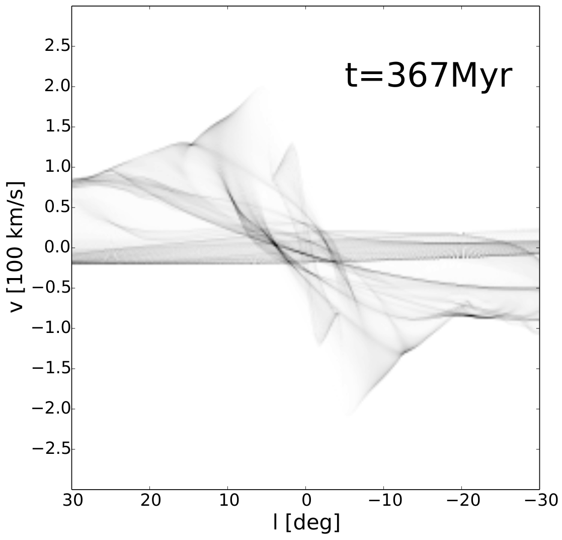
The Englmaier & Gerhard (1999) models we consider here quickly reach a steady state. Fig. 5 shows two snapshots of the model having pattern speed viewed with taken at two different evolutionary times. The features are almost identical, particularly outside the band we exclude from our fitting procedure.
To quantify this, we calculate the SMHD and ED between a synthetic plot at a fiducial evolutionary time, , with synthetic plots at different evolutionary times in the same simulation. Thus all synthetic plots considered in this section come from exactly the same potential, pattern speed and viewing angle ; only the time is allowed to vary. Fig. 6 shows the SMHD and ED between the fiducial snapshot at and all other snapshots in the same simulation. At the gas moves on purely circular orbits and the SMHD and ED are both very large. As the bar is gradually turned on over the first 150 Myr of the run, the gas settles into a distribution that approaches that of the fiducial snapshot at . While this is happening, the SMHD and ED both decrease from their high initial values to much lower values, reaching an approximate plateau starting from 300 Myr. Of course, at the special point both distances go to zero, but the sizes of the SMHD and ED in the plateau region away from this point provide lower bounds on the level of noise expected when we fit only relaxed, evolved versions of our models to mock data. Indeed, we will see below that varying one of the other parameters produces differences in SMHD and ED much greater than the height of the plateau.
We emphasize that, although this shows that the particular models we consider here do reach an effective steady state, the feature-fitting algorithm and SMHD distance of Section 4 do not require that such a steady state be reached. In the following subsections we make use of this effective steady state and compare mock data only to model snapshots taken at some time Myr long enough to allow the model to settle into a steady state; when fitting more general models with more than one pattern speed (Fux, 1999, e.g.,) one would have to include as a parameter to be fit.



5.2 Recovering the correct model parameters
Having eliminated time , we now turn to the more interesting question of how reliably one can identify the model parameters and . We construct three different mock datasets, shown in Figure 7. All are generated from a fiducial model having pattern speed viewed at Myr and angle , but differ in how the mock data are generated from that model. The first is constructed by projecting the fiducial model with and using the algorithm of Section 4.1 to extract features. The second is identical to the first, but projected with . The third is a modification of the first to which additional contaminating features have been added by hand.
For each mock dataset we construct models having in the range in steps of and in the range in steps of . For each model we project a single snapshot taken at with . Notice that none of our models use the “correct” values of Myr and from which the mock data are generated.
5.2.1 The basic test
The most basic test is given by checking how reliably the model parameters are recovered when the models adopt the correct projection law and the data are uncontaminated by misidentified features. The mock dataset used for this test is shown in Fig. 7(a). Figure 8 shows by how much models with assumed parameters differ from this mock dataset, as measured by SMHD, ED, and .
The plots demonstrate that when the projection law is correct (i.e., when there is no uncertainty associated with the chemistry of the ISM or radiative transfer), then all three distances can be used to locate the correct model; apart from some noisiness at low values of , they all descend smoothly to a minimum at (or very close to) the correct values of . Therefore if we start away from the correct model, e.g.,, with a pattern speed wrong by , then all three distances indicate in which direction we should move to get to the right model.
One point to note from these plots is that knowledge of the envelope alone suffices to identify the correct model among the restricted family of models we consider here. This is not true in general, a point to which we return in Section 5.3.
Another point is that the minimum in is much sharper than the minimum in either the SMHD or ED. measures the overlap between the data and model densities. Adjusting moves density around the plane. If the model density is similar to the observed one, but shifted in the plane, then the overlap between the two is low and tells us that the model is bad, despite the fact that a small adjustment to the model can lead to a significant improvement. This happens because compares only contents of the same bin, and does not take into account any cross-bin information. So, the width of the minimum in the is essentially measuring the width of the features. We discuss this further in Section 5.3.
None of the distances reach the value of zero because, as we noted above, the model used to produce the mock data set is not included, and also the evolutionary time between the two is different. For the SMHD the value of the minimum is above the value of the plateau in Fig.6, as are variations produced in the SMHD by all but the smallest variations of the parameters. Thus for this particular set of models we are justified in asserting that the time is a parameter that can be neglected if we are interested in recovering the value of the pattern speed and of the angle.


5.2.2 Effects of the projection law
The second test we run is the alpha test. In this test, we change the value of the exponent in the projection law (2) from to when building our mock dataset. All the other parameters retain the values they had in the basic test. Since a synthetic plot depends on how the projection of the gas is made, so too do the features, even though, as shown in Fig. 3, they do so only weakly when the projection is varied within physically plausible limits. The purpose of this test is to test whether we can recover the correct parameters if the models are built using the wrong projection law, which we can think of as a crude test of how sensitive the fit is to assumptions about ISM chemistry and radiative transfer processes.
When , the brightness temperature of the mock dataset does not depend linearly on the total column density, but on its third power instead. This is quite an extreme choice, probably well over the edge of the physically reasonable values. The mock dataset for this test is shown in 7(b). We see that the features change significantly from the basic test. In particular, some features disappear and are not visible anymore, while some features are enhanced. Features that disappear tend to be associated with velocity crowding, while features that survive tend to be associated with real overdensities in the gas distribution. The features for the are almost, but not exactly, a subset of the features for . Therefore in this test we are trying to match a mock dataset with much fewer features than our models have.
Fig.9 shows the result of the fitting. Again the model is clearly identified by the minimum SMHD, though the minimum is not as deep as found in the basic test when the correct was adopted. This happens because the best model now contains extra features that are not contained in the mock dataset. Nevertheless, the SMHD still does quite a good job in identifying the correct model. This test illustrates the robustness of the method: it shows that if we use the wrong radiative transfer approximation we should still be able to retrieve the correct model.
In this test, is clearly outperformed by SMHD (compare top and bottom rows in Fig. 9). does exhibit a minimum around the parameters of the correct model, but it is weaker than the minimum of the SMHD. is much flatter than SMHD when we are far from the correct model, with minima appearing in at in regions, while in the same regions SMHD points to the correct model. The explanation for this is that , by being heavily dependent on the intensities at each point, can fail to recognise that the overall morphology is similar.
As a by product of the fact that for the features diminish, this test shows that if for some other reason we fail to identify some features in the data, then we might still be able to find the correct model. In Fig. 10 we overlay the mock data of the alpha test with the correct parameters model and with two models that have one parameter, the angle, different from the correct value.
We do not plot the results for ED; they are unchanged from Fig. 8, as one might expect.
5.2.3 Effects of contamination
The last we run is the contamination test. The mock dataset for this is built by manually adding some extra features on top of the mock dataset for the basic test and it is shown in Fig.7(c). The purpose is to test the robustness of the method against the presence of spurious features in the data. These could represent some features that have been included in the data but are not really wanted, for example because they are caused by effects not taken into account by the models (if the connecting arm were due to magnetic fields and we do not include these in our simulations, this would count as contamination in this case). Fig. 11, top row, shows the results of this test. These are similar to the results for the alpha test, thus showing robustness of the method against presence of contamination. This test can be viewed as adding features as opposed to the alpha test were we are removing features. Thus the method is robust both against adding extra features and removing good ones.
5.2.4 Variations on SMHD
In Fig. 11, bottom row, we show the results of using the SMHD without the envelope using the contaminated dataset. It shows that even if one considers only the internal features, the correct model can still be identified, although the SMHD becomes more noisy. So, for this particular class of models, the internal features alone contain enough information to identify the correct model, albeit not as well as the envelope alone.
Finally, we have tested how the SMHD performs compares with unsymmetrized versions of the MHD. Given a choice between the two possibilities of using the MHD, the unsymmetrized version performs better than the symmetrized version either in the alpha test or in the contamination test, but not in both. At worst, the unsymmetrized MHD displays a shallower minimum, which is more difficult to identify, and weak secondary minima can appear. This agrees with our considerations in Sect. 4.2. The symmetrized version provides a compromise able to handle a wider range of situations.
5.3 Behaviour for families of models that are far from the fiducial model
Finally, as a more realistic test, we consider what happens when the models we search over are very different from the model from which the data are generated. We use mock data generated from the model given in Appendix A, with pattern speed and bar angle , projected with . As the form of the underlying potential of this galaxy model is very different to the Englmaier & Gerhard (1999) potentials that we try to fit to it, we do not expect these parameters to be retrieved correctly. The aim is instead to compare the quality of the best fits to the mock data according to the SMHD, ED and distances.
Fig. 12 shows the mock data used in this case, together with the models that minimize SMHD, ED and . It is clear that the model that reproduces the features best is, unsurprisingly, the one that minimizes the SMHD. The model that minimises the envelope distance matches the envelope very well, but fails to match the internal features well. It is evident that the model that minimises is entirely unsatisfactory.
In Fig. 13 we show how the distances vary with model parameters. The ED exhibits multiple minima, indicating degeneracy. In fact, it has a secondary minimum at the location of the best SMHD model, that is weaker than the main minimum. The is more flat, with weak minima here and there. If we consider that in this test the same approximation of radiative transfer physics is used for the data and the models, we argue that the situation would be even more hopeless than the plot indicates if one were trying to use without knowledge of the (unknown) correct model for the ISM chemistry and radiative transfer. This indicates that is not an appropriate goodness-of-fit measure, at least not until one understands the latter. In Sect. 7 we come back to this topic and discuss the reasons for this behavior.


6 Application to Real Data


Having applied the SMHD to mock data, we now test how well it works when applied to to the features in the real data identified in Section 2. We do not produce any new models here, but instead compare the fits provided by three of the best models from the literature: the standard model of Englmaier & Gerhard (1999); that of Bissantz et al. (2003) (their Table 1); and the best overall model of Rodriguez-Fernandez & Combes (2008), the rotation curve of which is shown in their Fig. 6.
The model of Englmaier & Gerhard (1999) is stationary in a frame that corotates with the bar pattern speed of ; there are no spiral arms. The model of Bissantz et al. (2003) is nonstationary, as it includes a bar and a spiral arm component rotating respectively at and . Rodriguez-Fernandez & Combes (2008) includes two bars, a big bar and a smaller nuclear bar making a constant angle of with the first, both rotating at the same pattern speed . It has no spiral arms.55 5 In order to reproduce the rotation curve plotted in Fig. 6 of Rodriguez-Fernandez & Combes (2008) we found that we had to replace the exponent of in their expression (9) for with an exponent of . We assume that this is a typographical error in the paper, even though it means that their boxy Gaussian bulge is actually a boxy exponential bulge.
Our reconstructions of snapshots of the density profiles of these three models are shown in Fig. 2. The corresponding projected distributions for a viewing angle of are shown in Fig. 14. We have compared our density and plots with the appropriate figures from the original papers and were find that the location of the features agree very well indeed. This agreement is surprising, given that our models are based on an Eulerian grid simulation, whereas Englmaier & Gerhard (1999) and Bissantz et al. (2003) used a SPH code while Rodriguez-Fernandez & Combes (2008) use a sticky-particle code. It is particularly remarkable that we reproduce the latter so well: sticky particle simulations in principle solve different fluid equations than our FS2-based method. The fact that the three methods give similar results on the scales we are interested in corroborates our claim that we should first try to match the observational data with simple models, so as to reproduce the overall structure, and only later move to more refined models to reproduce the details. When the gross structure is not known, it is in general a pointless exercise to add effects if they turn out to be of secondary importance.
For each of our three reconstructions, we use the algorithm of Section 4.1 to extract the features. These are overlaid on the right column of Fig. 14 with the features extracted by eye from the observations (Section 2). Unfortunately, these plots highlight the shortcomings of current models. The main problems are:
- 1.
no model is able to reproduce the high velocity peaks at and . In particular the Rodriguez-Fernandez & Combes (2008) model has a very low peak velocity of less than .
- 2.
no model reproduces the huge forbidden velocities at and . Rodriguez-Fernandez & Combes (2008) do better than the others in this, but large uncovered portions remain.
- 3.
broad features, such as the 3-kpc arm, are not reproduced well by the Englmaier & Gerhard (1999) or Bissantz et al. (2003) models. The more recent models of Rodriguez-Fernandez & Combes (2008) do a better job here, providing a good fit to both the near- and far-side 3kpc arms.
- 4.
the very complicated central structure, for example the vertical features, is not reproduced in any model.
As a very limited test of whether one could easily improve on this situation, we fit the same set of models used in Sect. 5, based on our reconstruction of the Englmaier & Gerhard (1999) potential, to the real Galaxy features. As before the models have in range , in range , all viewed at evolutionary time and projected with . To allow the models some extra freedom we allow an extra parameter that scales all velocities of the gas. When velocities are scaled such that , the other quantities scale in the following way: , , , .
In Fig. 15 we show the results of minimising the SMHD (top row) and ED (bottom row). We note that the graphs are smooth and not dominated by noise. The best fits are different according to the two methods. In Fig. 16, panel (a) and (b), we show the best fits according to SMHD and ED respectively. The parameter values for these are the overall minima in the graphs of Fig. 15. These are , , for the best SMHD, and , , for the best ED model. Unfortunately, we believe that both should be considered unsatisfactory, as in each important ingredients are missing. No model is able to reproduce high forbidden velocity and, at the same time, the high velocity peaks, and features are also not reproduced well. Interestingly, in the best ED model a weak vertical feature appears at negative velocities, approximately at , . To the best of our knowledge, it is the first time that such a feature appears in a synthetic plot and suggests that could explain this feature if we had the right potential. In the face-on view of the Galaxy, this feature corresponds to an offset shock lane.
In panel (c) of Fig. 16 we show a further model, labelled “GE”, that we found in our reconstruction of Bissantz et al. (2003) potential for , , . This model has an envelope that matches the observed one amazingly well, filling the right forbidden velocities region. If one were to judge this model only from the envelope, akin to what Weiner & Sellwood (1999) did, this would be considered a very good one. We do not consider this to be a particularly good model, however. The internal features are completely wrong, except close to the Molecular Ring region. The very central region is almost featureless, and it exhibits nothing similar to the 3kpc arm, the connecting arm or the CMZ. This model illustrates for the real case that the envelope is not enough to constrain the Galaxy potential, and in this work we argue that the next piece of information that should be taken into account is given by the internal features.


7 Discussion
7.1 Comparison of SMHD with Envelope Distance and , and their limitations
Apart from “by-eye” comparisons, the two most widely used ways of fitting models to observed distributions have been some variations of the Envelope Distance (Weiner & Sellwood, 1999; Englmaier & Gerhard, 1999, equ. 7, e.g.,) and (Pettitt et al., 2014, equ. 6, e.g.,).
While the ED is very robust with respect to changes in radiative transfer physics, it has the obvious disadvantage of neglecting all the information coming from internal features; thus, the degeneracy of the problem is increased. We know, for example, that it is possible to reproduce any terminal velocity curve in the and quadrants by means of gas moving on purely circular orbits. In Sect. 5.3 we have shown that the Envelope Distance can be degenerate when the SMHD is not, so the latter can provide a better-fitting model than the former. In Sec. 6 we have shown a model that fits well the envelope for the real data, but it is overall unsatisfactory as it fails to fit the internal features. The internal features must certainly contain additional information and should be taken into account when comparing the data with the models. In Fig. 11 we give an example of a case in which internal features alone are sufficient to identify the correct galaxy model, albeit not quite so securely as when the envelope is known as well.
In constrast, makes full use of all of the available data, but it suffers from serious drawbacks when one tries to use it to contrain the geometry and dynamics of the Galaxy. One of the main concerns is that only compares model versus observed intensities in the same bin and does not take into account any cross-bin information. If, for example, a model displays features that are very similar to the observational features, but are slightly misplaced in the plane, the distance can suggest that the model is terrible; in the most extreme case, even a bland, featureless model might be a formally better fit, while visual inspection would suggest that the models are actually quite good. This means that raw fails to capture the essence of what is important in comparing model and data in this case. This is what happens in the situation of Sect. 5.3, where we have shown that provides unsatisfactory fits even when the same approximation of radiative transfer physics is used for the data and the models.
has other drawbacks. It is computationally expensive. As it is entirely dependent on local intensities, its use necessarily requires detailed modelling of radiative transfer physics, chemistry and gas dynamics all at the same time, which is very time consuming. On the other hand, models need to be cheap to test because the space of possible models is large. We would like to know not only the pattern speed and orientation of the bar, but also its mass, length, axis ratio, and possibly more. Computational expense is the reason why Pettitt et al. (2014), despite having a full radiative transfer model, did not use it when fitting the data and relied on a very simplified radiative transfer model akin to ours. is clearly not the best choice in situations such as the alpha test in Sect. 4, where everything in the model is correct except the radiative transfer modelling.
Current models of the gas flow in the Milky Way (Sect. 6) are unsatisfactory. We argue that the sensible way of addressing this is to note that, as we found in Sect. 4, the features in the distribution give valuable constraints on the Galactic potential that are largely independent of the details of ISM chemistry or radiative transfer. Therefore one should first build models that match well the broad morphology of the observations to narrow down the potential, and only later refine this to match the details. As we’ve shown in Sect. 6, the envelope is too degenerate for such a task, even in the case of real data: a model with that reproduces only the envelope well can still be unsatisfactory.
Thus one should use the SMHD or similar scheme to locate the range of broadly acceptable potentials and pattern speed(s). Only when this large-scale structure has been constrained it does make sense to switch to more sophisticated models that include chemistry and proper radiative transfer modelling. We believe that (or similar) should play an important role only in this last step. An alternative to that might be worth considering in this last step is the “earth mover distance” (Appendix B).
We emphasise that, unlike , the SMHD is a purely qualitative measure that cannot sensibly be used to provide formal uncertainties on the parameters of models that fit the observations. Given the present ambiguity as to the overall form of the Galactic potential, we would argue that any such attempt would be misleading.
7.2 Identification of “features”
The SMHD returns a number that quantifies the dissimilarity of two sets of features in the plane: the higher the number, the more dissimilar the features. The procedure for identifying features in data and models requires some remarks. For models, we have a fully automatic algorithm (Sect 4.1) that, given a model distribution returns the features as 1-pixel wide lines. The features we identified as being important are bright ridges and the envelope. Therefore, the algorithm simply detects ridges and envelope given a model distribution.
7.2.1 Features in data
It is natural to ask whether the data could be analysed in the same way as the models to extract features automatically. Unfortunately, this turned out to be problematic: unlike our simple, smooth hydrodynamical models, the real data exhibit substructures due to clumpiness that are identified as spurious ridges by our ridge-detection algorithm. Moreover, the analysis of features in the data often involves looking at different latitude slices, and each feature may require a special analysis and considerable work as the example of the Far side 3kpc arm (Dame & Thaddeus, 2008) shows. This is clearly beyond our algorithm’s capabilities and requires the skills of experienced astronomers. For this reason, we rely on human wisdom for the identification of features in the real data.
7.2.2 Suitability of models
Any model for the gas flow comes with a series of implicit or explicit simplifying assumptions. In the present paper our gas models are 2D; we neglect the vertical dimension, which could also play an important role. We do not include heating and cooling processes due to a variety of sources, such as supernovae explosions and stellar winds. Modeling the gas as a smooth fluid means neglecting all the grainy structure, such as individual clouds with peculiar velocities. Indeed, the crude modelling with the Euler equation is applicable only in a coarse-grained sense, and does not take into account explicitly local turbulence, temperature variations and multiphase nature of the ISM. Lastly, we neglect the self-gravity of the gas that could be important especially near shocks or other structures where gas accumulates. There is nothing to prevent us from applying the SMHD method to more (or less) sophisticated models, as long as they produce smooth distributions; as discussed above, we argue that for finding the large-scale structure of the gas distribution, which is currently poorly understood, the simpler the model the better.
7.2.3 Possible extensions
The method can easily be adjusted to incorporate our beliefs about how features are generated. For example, one could argue that the envelope is of different nature than the internal features, and therefore we should calculate two separate SMHDs, one that matches only the envelopes and one matching only the internal features. Another example is provided by the fact that, because of absorption, for many features we know whether they are caused by material in front of the Galactic Center (for example the 3kpc arm) or behind it (Cohen, 1975, for example, the arm, see ). It would therefore be natural to match features that we know are in front of the GC with features that are in front also in the models. A further example is provided by the tilt of the Inner Galaxy (Burton et al., 1992): if we believe that a part of the Galaxy – for example the inner nuclear disk – is tilted, then we would like to match observational tilted features only with features that are produced within the corresponding region in the models. This is straightforward to do by fitting multiple SMHDs.
As an illustrative example, to incorporate the information on whether features are in front or behind the GC, we can proceed as follows. We divide data features in three sets: are features we know lie in front of the GC, those that lie behind, those whose position is unknown. Model features are divided only in two sets, and , as for each model feature we always have information on its position with respect to the GC. Then a suitable definition of SMHD that takes into account the new information (and reduces to the previous definition in absence of new information) is:
| (8) |
where
| (9) |
and
| (10) |
Other prior information could be taken into account in a similar way, dividing the feature in different sets and defining the rules by which these sets should be matched.
8 Conclusion
We have proposed a new way of fitting model distributions to observations. We have argued that one can separate the effects of the large-scale dynamics and structure of the Galaxy from those due to details of radiative transfer and chemistry. Based on this, our SMHD provides a way of measuring distances between features in models versus corrsponding features in the observations.
We have tested the ability of our method to fit models to mock data generated under a variety of conditions, and have compared it to alternative methods. To the best of our knowledge, this is the first time that the ability of such methods to retrieve model parameters by fitting to distributions has been investigated systematically. We have also explicitly demonstrated the importance of internal features in the plots, that have been the basis for comparison of plots to observations by many authors who have run simulations.
We find that our feature-based SMHD method works well and is much more robust than other methods. It works in cases in which the assumed (crude) radiative transfer model is wrong or when the data are contaminated. The Envelope Distance, as expected, is often degenerate in cases where the SMHD is not, as the ED exploits only a small part of the information available in the data. We found this to be true both for mock and real data. On the other hand, we found to be unsuited to the task of matching longitude-velocity diagrams when this requires exploration of a huge parameter space. It works well only in the very vicinity of the correct solution, and at the price that all pieces of physics are taken into account in producing synthetic plots, including those that can be disentangled from the dynamics of the gas. The main reasons for this behaviour are (i) that fails to take into account cross-bin information, which means that it tends to favour models that have little structure. (ii) its use is computationally expensive as it requires modelling the chemistry of the ISM and carrying out full radiative transfer calculations. We argued that such calculations are unnecessary if all one wants to do is to constrain the Galaxy’s gravitational potential and the large-scale distribution of its gas. Given that current dynamical models for the Galaxy appear to be far from the truth and that fitting the envelope alone is not enough, one should first constrain the gross morphology found in data using, for example, SMHD, and only later, once one has almost nailed down the potential, turn on more details of physics and finally use to take advantage of its statistical interpretation.
Our method is computationally inexpensive because it relies on simple hydro simulations and avoids the need to model chemistry or to carry out sophisticated radiative-transfer modelling. This makes it suitable for carrying out large, systematic scans of model parameter space. It is easily applied to time-dependent simulations. It can be used to test the reality of observed features (by comparing fits with and without the feature present) and can naturally be extended to test hypotheses, such as “this feature belongs to a foreground spiral arm” or “that feature is the trace of the orbit” with a little extra analysis of the internal dynamics of the models used for comparison. It does, however, require some work in that it relies on features being identified “by hand” in the data. It also requires that the models used for comparison are smooth enough to allow the feature extraction algorithm to work; sophisticated models that produce clumpy structures would probably not be suitable.
We have reconstructed, and reanalysed by applying our method, some of the best models from the literature that were constructed to fit the Dame et al. (2001) and Kalberla et al. (2005) data on the Milky Way, but find that they produce surprisingly poor fits. We have made an initial attempt to fit the data, but our family of models was too limited. We were able to find a model that reproduces the envelope of the emission accurately, but this fails in explaining the internal structure of the data; nevertheless, this demonstrated only that the envelope alone is insufficient to constrain the Galactic potential. As an interesting by product, we found that the large-scale morphology is not very sensitive on the simulation method. The sticky-particles code used by (Rodriguez-Fernandez & Combes, 2008) gave a large-scale morphology very similar to our grid-based code, despite the fact that in principle it solves a different set of hydrodynamical equations. This corroborates our claim that to find the gross morphology of the Galaxy one should focus on simple hydrodynamical models.
The problem is now that of finding a sufficiently general class of model potentials to use in the comparison. One possibility is to express the first few multipole moments of the Galaxy’s mass density distribution in terms of splines and to develop an automatic scheme for adjusting the spline weights to minimize the SMHD distance. A good model should also take into account constraints coming from different sources, for example infrared data from the 2MASS survey (Skrutskie et al., 2006) and the correlations expected between the three-dimensional distribution of gas and independent results on the three-dimensional distribution of dust (Marshall et al., 2006; Green et al., 2014; Sale & Magorrian, 2014, e.g.,).
Acknowledgments
We are indebted to James Binney for his helpful insights at all stages of the development of this work. MCS thanks Maria Colombo for suggesting the use of EMD and acknowledges support from a Clarendon Fund Scholarship. JM acknowledges support from STFC and ERC.
References
- Athanassoula (1992) Athanassoula E., 1992, MNRAS, 259, 345
- Athanassoula (2012) Athanassoula E., 2012, in European Physical Journal Web of Conferences. p. 6004
- Baba et al. (2010) Baba J., Saitoh T. R., Wada K., 2010, PASJ, 62, 1413
- Bally et al. (1987) Bally J., Stark A. A., Wilson R. W., Henkel C., 1987, ApJS, 65, 13
- Bally et al. (1988) Bally J., Stark A. A., Wilson R. W., Henkel C., 1988, ApJ, 324, 223
- Bania (1977) Bania T. M., 1977, ApJ, 216, 381
- Binney et al. (1997) Binney J., Gerhard O., Spergel D., 1997, MNRAS, 288, 365
- Binney et al. (1991) Binney J., Gerhard O. E., Stark A. A., Bally J., Uchida K. I., 1991, MNRAS, 252, 210
- Binney & Merrifield (1998) Binney J., Merrifield M., 1998, Galactic Astronomy. Princeton University Press
- Bissantz et al. (2003) Bissantz N., Englmaier P., Gerhard O., 2003, MNRAS, 340, 949
- Blitz & Spergel (1991) Blitz L., Spergel D. N., 1991, ApJ, 379, 631
- Burton et al. (1992) Burton W. B., Elmegreen B. G., Genzel R., eds, 1992, The galactic interstellar medium
- Canny (1986) Canny J., 1986, IEEE Trans. Pattern Anal. Mach. Intell., 8, 679
- Cohen (1975) Cohen R. J., 1975, MNRAS, 171, 659
- Dame et al. (2001) Dame T. M., Hartmann D., Thaddeus P., 2001, ApJ, 547, 792
- Dame & Thaddeus (2008) Dame T. M., Thaddeus P., 2008, ApJ, 683, L143
- de Vaucouleurs (1964) de Vaucouleurs G., 1964, in Kerr F. J., ed., IAU Symposium Vol. 20, The Galaxy and the Magellanic Clouds. p. 195
- Dehnen & Binney (1998) Dehnen W., Binney J., 1998, MNRAS, 294, 429
- Dobbs et al. (2011) Dobbs C. L., Burkert A., Pringle J. E., 2011, MNRAS, 417, 1318
- Dubuisson & Jain (1994) Dubuisson M.-P., Jain A. K., , 1994, A Modified Hausdorff Distance for Object Matching
- Dwek et al. (1995) Dwek E. et al., 1995, ApJ, 445, 716
- Englmaier & Gerhard (1999) Englmaier P., Gerhard O., 1999, MNRAS, 304, 512
- Ferrière (2001) Ferrière K. M., 2001, Reviews of Modern Physics, 73, 1031
- Fux (1999) Fux R., 1999, A&A, 345, 787
- Fux (2004) Fux R., 2004, in Alfaro E. J., Pérez E., Franco J., eds, Astrophysics and Space Science Library Vol. 315, How Does the Galaxy Work?. p. 213
- Gerhard (2002) Gerhard O., 2002, in Da Costa G. S., Sadler E. M., Jerjen H., eds, Astronomical Society of the Pacific Conference Series Vol. 273, The Dynamics, Structure & History of Galaxies: A Workshop in Honour of Professor Ken Freeman. p. 73
- Gerhard & Vietri (1986) Gerhard O. E., Vietri M., 1986, MNRAS, 223, 377
- Green et al. (2014) Green G. M. et al., 2014, ApJ, 783, 114
- Jenkins & Binney (1994) Jenkins A., Binney J., 1994, MNRAS, 270, 703
- Kalberla et al. (2005) Kalberla P. M. W., Burton W. B., Hartmann D., Arnal E. M., Bajaja E., Morras R., Pöppel W. G. L., 2005, A&A, 440, 775
- Lee et al. (1999) Lee C. W., Lee H. M., Ann H. B., Kwon K. H., 1999, ApJ, 513, 242
- Lindeberg (1996) Lindeberg T., 1996, International Journal of Computer Vision, 30, 465
- Liszt (2008) Liszt H. S., 2008, A&A, 486, 467
- Liszt & Burton (1980) Liszt H. S., Burton W. B., 1980, ApJ, 236, 779
- Machida et al. (2009) Machida M. et al., 2009, Publications of the Astronomical Society of Japan, 61, 411
- Marshall et al. (2009) Marshall D. J., Fux R., Robin A. C., Reylé C., 2009, in The Evolving ISM in the Milky Way and Nearby Galaxies.
- Marshall et al. (2006) Marshall D. J., Robin A. C., Reylé C., Schultheis M., Picaud S., 2006, A&A, 453, 635
- Merrifield (2004) Merrifield M. R., 2004, in Clemens D., Shah R., Brainerd T., eds, Astronomical Society of the Pacific Conference Series Vol. 317, Milky Way Surveys: The Structure and Evolution of our Galaxy. p. 289
- Mulder & Liem (1986) Mulder W. A., Liem B. T., 1986, A&A, 157, 148
- Oort (1977) Oort J. H., 1977, Comments on Astrophysics, 7, 51
- Peters (1975) Peters III W. L., 1975, ApJ, 195, 617
- Pettitt et al. (2014) Pettitt A. R., Dobbs C. L., Acreman D. M., Price D. J., 2014, MNRAS, 444, 919
- Rodriguez-Fernandez & Combes (2008) Rodriguez-Fernandez N. J., Combes F., 2008, A&A, 489, 115
- Rougoor (1964) Rougoor G. W., 1964, Bulletin of the Astronomical Institutes of the Netherlands, 17, 381
- Rougoor & Oort (1960) Rougoor G. W., Oort J. H., 1960, Proceedings of the National Academy of Science, 46, 1
- Rubner et al. (2000) Rubner Y., Tomasi C., Guibas L. J., Guibas L. J., 2000. pp 99–121
- Sale & Magorrian (2014) Sale S. E., Magorrian J., 2014, MNRAS, 445, 256
- Sawada et al. (2001) Sawada T. et al., 2001, ApJS, 136, 189
- Shane & Bieger-Smith (1966) Shane W. W., Bieger-Smith G. P., 1966, Bulletin of the Astronomical Institutes of the Netherlands, 18, 263
- Shetty & Ostriker (2008) Shetty R., Ostriker E. C., 2008, ApJ, 684, 978
- Shu (1992) Shu F. H., 1992, Physics of Astrophysics, Vol. II. University Science Books
- Skrutskie et al. (2006) Skrutskie M. F. et al., 2006, AJ, 131, 1163
- Sobel & Feldman (1968) Sobel I., Feldman G., 1968, A 3x3 Isotropic Gradient Operator for Image Processing, Never published but presented at a talk at the Stanford Artificial Project
- Stark & Bania (1986) Stark A. A., Bania T. M., 1986, ApJL, 306, L17
- Tasker (2011) Tasker E. J., 2011, ApJ, 730, 11
- van Albada et al. (1982) van Albada G. D., van Leer B., Roberts Jr. W. W., 1982, A&A, 108, 76
- van der Kruit (1970) van der Kruit P. C., 1970, A&A, 4, 462
- Weiner & Sellwood (1999) Weiner B. J., Sellwood J. A., 1999, ApJ, 524, 112
- Zhang & Suen (1984) Zhang T. Y., Suen C. Y., 1984, Commun. ACM, 27, 236
Appendix A A Potential
Here are the details of the potential used in the generation of the mock data in Section 5.3. The potential is inspired by Dehnen & Binney (1998) models. It is made by 3 components: Bar, Disk, Halo. Table 1 shows the value of the parameters used. The potential is steady in a frame that rotates pattern speed .
Bar
The density distribution generating the potential of the bar is given by
| (11) |
where
To fully specify the bar potential we therefore need 4 parameters: the central concentration , inner slope , major axis and axis ratio . Equivalently, we can specify the total mass instead of the central concentration .
Disk
The density distribution of the disk is exponential. It has zero thickness, and the surface mass density is given by
| (12) |
To fully specify the disk potential we need 2 parameters: the radius and the central surface mass density .
Halo
The Halo potential is logarithmic.
| (13) |
To fully specify the halo potential we need 2 parameters: the radius and the circular velocity at infinity .
| Bar | ||||
| Disk | ||||
| Halo | ||||
| Omega | ||||
| Phi | 35 ∘ | |||
Appendix B Earth Mover Distance
The Earth-mover distance is a way of quantifying the dissimilarity of two distributions. Intuitively, given two distributions, one can be seen as a collection of piles of earth spread in space, the other as a collection of of holes in the same space. The amount of earth at each point can be any positive real number. The EMD measures the minimal amount of work needed to fill in the holes with earth taken from the piles. A unit of work corresponds to transporting a unit of earth by a unit of ground distance, which in our case would be a metric suitably defined in the plane. The earth contained in one pile can be shared among many different holes if this solution requires less work than other alternatives. More details on this distance can be found for example in Rubner et al. (2000).
As noted in Section 4.2, EMD is an option that we initially found intuitively appealing for comparing features. In this case, the idea is to apply the EMD to binary images such as panel (h) in Fig. 4. The amount of earth is 1 at pixels corresponding to features, and zero otherwise. The dissimilarity between model features and data features is quantified by the minimal amount of work needed to turn the model features into data features (or vice versa). When used in this way, the EMD turned out to underperform the much simpler SMHD; if anything, the EMD was actually too clever in matching features from one image to the other, with the result that the variation of EMD with and had spikes and false minima, and was much noisier than either the SMHD or envelope distances.
Nevertheless, if one were faced with carrying out full radiative-transfer modelling, the EMD used in a qualitatively different way might be reconsidered as an alternative to . The idea in this case would be to use the Earth Mover Distance to compare two full distributions, such as panel (a) in Fig. 4. The amount of earth would then be the brightness temperature at each pixel, which would not constrained to be either 0 or 1. The potential advantage of EMD used in this way would be that it avoids one of main problems, namely that of ignoring cross-bin information. We therefore suspect that it might be useful in cases where one were trying to fit the details of the chemistry and radiative transfer as well as the potential. In exploratory tests we found that EMD applied to the full distributions performed well in retrieving parameters when the rule (2) used to project the models was identical to that used to generate the mock data. As the EMD used in this way is strongly dependent on the intensities at each point, it requires that a full radiative-transfer model be included, however.