Low-density homogeneous symmetric nuclear matter: disclosing dinucleons in coexisting phases
Abstract
The effect of in-medium dinucleon bound states on self-consistent single-particle fields in Brueckner, Bethe and Goldstone theory is investigated in symmetric nuclear matter at zero temperature. To this end, dinucleon bound state occurences in the and channels are explicitly accounted for –within the continuous choice for the auxiliary fields– while imposing self-consistency in Brueckner-Hartree-Fock approximation calculations. Searches are carried out at Fermi momenta in the range fm-1, using the Argonne bare nucleon-nucleon potential without resorting to the effective mass approximation. As a result, two distinct solutions meeting the self-consistency requirement are found with overlapping domains in the interval , corresponding to mass densities between and g cm-3. Effective masses as high as three times the nucleon mass are found in the coexistence domain. The emergence of superfluidity in relationship with BCS pairing gap solutions is discussed.
pacs
21.65.-fNuclear matter and 21.45.BcTwo-nucleon system and 21.65.MnEquations of state of nuclear matter1 Introduction
Dinucleon formation, pairing, clustering and condensation in nuclear media have been subjects of considerable research during the past few decades motivated by their role in heavy-ion collisions, collapsing stars, weakly bound nuclear systems and critical phenomena [1, 2]. Even in their simplest conceptions, nuclear matter models may become exceedingly complex systems featuring strongly-interacting Fermions over a broad range of conditions. Densities may vary from highly diluted systems, as in nuclear halos or envelopes of core-collapse supernovae, up to a few times the saturation density, as in the core of neutron stars. The isospin asymmetry can also vary from zero, as in symmetric nuclear matter, up to unity, as in pure neutron matter thought to prevail in the interior of neutron stars. Temperature can also be subject to wide variations from zero up to a few hundreds of MeV.
Among the various approaches to study interacting nucleons systems, the Brueckner-Hartree-Fock (BHF) approximation can be regarded as a reasonable starting point to investigate homogeneous infinite nuclear matter [3, 4]. This approximation embodies important information upon which higher order corrections can be incorporated [5]. However, it has long been recognized that bound states in BHF approximation signal the onset of superfluidity, phenomenon which needs to be investigated within a much broader framework [6]. Beyond this limitation, the question remains as to whether it is feasible to find self-consistent single-particle (sp) fields in infinite nuclear matter within BHF, accounting simultaneously for dinucleon bound states. In this work we address this issue by providing an explicit account for dinucleon bound states in the and channels, expressed as isolated poles of the matrix on the real axis below the continuum threshold, while seeking self-consistency in the sp potential. We have avoided the use of the effective mass approximation to represent the sp fields, aiming to rule out potential sources of ambiguities in our findings. Additionally, the sp momentum distribution follows a normal Fermi distribution, namely , with the Fermi momentum. As a consequence we obtain two distinct solutions satisfying the self-consistency requirement in the range , i.e. matter densities between and fm-3, corresponding to mass densities of and g cm-3, respectively. To investigate and resolve these features, special measures were needed to control singularities implied by bound states. Considering that at very low densities hole-hole ladder contributions become weak [7] due to the limited phase space they act upon, the results we obtain for nuclear densities below based only on particle-particle (pp) contributions become reasonably justified within BHF alone, namely as long as effects associated with superfluidity are neglected. In any case, taking the present results as a baseline, the inclusion of hole-hole propagation beyond Brueckner ladder diagrams would need to be reassessed in another work.
Nuclear matter properties have been extensively investigated in the framework of the Brueckner-Bethe-Goldstone (BBG) theory based on the hole-line expansion for the ground state energy [8]. Here the Goldstone diagrams are grouped according to their number of hole lines, with each group summed up separately. The summation of the two-hole-line diagrams yields the usual BHF approximation, where the two-body scattering matrix in nuclear matter is calculated self-consistently with the sp energy spectrum. Although the sp potential is introduced only as an auxiliary quantity, its choice conditions the rate of convergence of the expansion for the binding energy. In ref. [9] it has been reported that the continuous choice [10, 11, 12] for the auxiliary potential provides better convergence over the so called standard choice, where the sp potential is set to zero above the Fermi energy. Hence, we shall use the continuous choice to investigate the role of dinucleon bound states during the search for self-consistent sp potentials.
This paper is organized as follows. In sec. 2 we outline the theoretical background upon which we address self-consistency in nuclear matter within the BHF approximation. In sec. 3 we succinctly describe special measures aimed to control numerical instabilities, particularly the treatment of dinucleon bound-state poles of the matrix on the real axis. We also address the existence of multiple roots in the energy denominator of the propagator and describe procedures to handle sharp integrands. In sec. 4 we present and discuss solutions for the self-consistent sp fields, associated nuclear matter binding and effective masses. We also discuss spatial properties of dinucleons as well as some immediate implications of the sp fields when applied in the context of pairing gap equations for superfluid states. In sec. 5 we present a summary of the work, draw its main conclusions and outlook.
2 Framework
In BBG theory for symmetric nuclear matter the matrix depends on the density of the medium, characterized by the Fermi momentum , and a starting energy . To lowest order in the BHF approximation for nuclear matter in normal state, when only two-body correlations are taken into account, the matrix satisfies
| (1) |
with the bare interaction between nucleons, the sp energy of nucleon (), and the Pauli blocking operator which in normal BHF takes the form
The solution to eq. (1) enables the evaluation of the mass operator
| (2) |
where is the total momentum of the interacting pair, , and
| (3) |
the sp energy defined in terms of an auxiliary field . The nucleon mass is taken as the average of proton and neutron masses. In the BHF approximation the sp potential is given by the on-shell mass operator,
| (4) |
self-consistency requirement which can be achieved iteratively. In the continuous choice this condition is imposed at all momenta [13].
In momentum representation the BHF equation takes the explicit form
| (5) |
where accounts for the particle-particle (pp) potential
| (6) |
with
| (7) |
Here , corresponding to the cosine of the angle between and , with the relative momentum of intermediate states.
3 Methods
A standard procedure to solve the non-linear system of eqs. (1-4) is by iterative feed-backing, where the auxiliary field is initially unknown. Each cycle begins with the definition of an initial guess for , which allows solving eq. (1) for any and . The series of cycles may be started with , to obtain all -matrix elements needed for the evaluation of in eq. (2). The real part of defines a new sp field, , which becomes the guess for a new cycle. The procedure is repeated until differences between consecutive solutions for meet some convergence criterion. Although this self-consistent scheme works well at normal densities, convergence becomes more difficult as diminishes below 0.8 fm-1, feature manifested by instabilities in the evaluation of the on-shell mass operator. To attenuate these instabilities we cite refs. [14], for example, where self-consistency at low densities was reached by reducing the number of mesh points for the Fermi-motion integral in eq. (2). With such numerical compromise it was possible to attenuate sudden fluctuations of the integrand, which at the time of the work had no identifiable cause. These solutions are used to calculate nucleon-nucleon (NN) effective interaction, i.e. off-shell matrix, to evaluate momentum-space optical model potentials for nucleon scattering off nuclei.
Aiming to obtain genuine self-consistent solutions for the sp mean fields over a wide density regime, particularly at low densities, a refinement of numerical techniques becomes crucial to control instabilities during the iterative process. In the following we describe the most relevant constructions toward this end.
3.1 Multiple roots
To solve eq. (5) we take the angular average of the energy denominator,
| (8) |
where . Additionally, if the Pauli blocking operator is angle-averaged the multi-channel coupling among different total angular momentum states become disentangled. In ref. [15] this is referred to as ratio-of-average approximation, which in this study constitutes a starting point. After partial wave expansion, eq. (1) for uncoupled channels reads
| (9) |
where
| (10) |
A similar equation is obtained in the case of coupled states. The above integral equation can be solved numerically with the use of numerical quadrature and matrix inversion. However, caution is called for in the treatment of the zeros of the energy denominator. Indeed, the fact that is a growing function in does not necessarily imply the same trend for the two-particle energy . Hence, more than one root in the energy denominator of eq. (9) cannot be ruled out.
To clarify this point consider the angle-averaged potential in eq. (8) evaluated using a two-point Gaussian quadrature. Thus
| (11) |
where . Single zeros (or none) in are guaranteed if is an ever growing function in , namely . Hence,
| (12) |
where stands for derivative of with respect to its argument. Assuming positive for all , the validity of the above inequality depends on the sign of the third term. Only if is quadratic in the above inequality is met, which is not the case in actual solutions.
Therefore, even if the genuine sp self-consistent fields result as monotonic functions in the momentum space, multiple roots cannot be ruled out in the energy denominator of the propagator. This aspect, in the context of the integral equation for the matrix, can be handled as outlined in Appendix A.
3.2 Fermi-motion integrals
The evaluation of the sp fields, , involves the summation of on-shell -matrix elements while keeping the momentum of one of the particles below the Fermi surface. Explicitly,
| (13) |
Here , the energy is evaluated on-shell (), denotes spin, isospin and angular momentum states, and accounts for their degeneracy and for geometric factors.
For most NN states the integration within the Fermi sphere involves well behaved integrands, as given by the on-shell . However, extra measures becomes unavoidable when considering the and channels. This is because during the evaluation of the momentum integral in eq. (13), exceedingly large -matrix elements may occur, stemming from NN bound states in these S and D channels. Indeed, any matrix element with starting energy near these bound states will lead to large contributions. To illustrate the occurrence of these states, let us define
| (14) |
with the pp propagator in eq. (9) and denoting a particular NN channel. In fig. 1 we plot for (thin curves) and (thick curves) channels as a function of , with the threshold energy allowed by Pauli blocking. For this example we have chosen fm-1. Solid, long- and short-dashed curves correspond to total pair momenta , 0.05 and 0.1 fm-1, respectively. A singularity of in channel is identified by the zero of . As observed, the deuteron channel exhibits bound states in all three cases, while for the channel they occur over a narrower interval in . Hence, if during the evaluation of the integrals in eq. (13) a configuration of total momentum and starting energy happens to be near (or at) one of these singular points, large (or undefined) contributions become unavoidable. This feature becomes a major source of numerical instabilities if not handled properly.

To evaluate the mass operator we use the alternative set of variables and defined by [16]
| (15a) | ||||
| (15b) | ||||
Thus, . Therefore the on-shell mass operator, eq. (13), is now expressed as
| (16) |
To be consistent with the angle-averaged pp energy, the starting energy is evaluated according to eq. (10). With this set of integration variables, for given , and , the limits of integration on become
where . In the case of , the integration ranges from , up to . In fig. 2 we illustrate the four possible shapes in the plane where the integral on takes place, depending on relative to .

The above choice of coordinates facilitates tracking and control of dinucleon singularities. Indeed, for constant the eigenenergy of an eventual dinucleon bound-state pole remains unchanged while the integration on takes place. Additionally, considering the spectral representation of when bound states occur [17], its behavior for near the energy of the bound state becomes
| (17) |
with the eigenfunction at the pole, the bare potential in the corresponding channel, and the Pauli blocking operator. This analytic property allows us to safely state that the mass operator, expressed as an integral over momenta of with isolated singularities, should be finite. The rationale behind this statement is that if simple poles occur, the integration over of the singular part of in eq. (16) reduces to
| (18) |
Note that the numerator is bound. Expanding the denominator to first order in around its zero, which we assume inside the interval of integration, the contribution around the singularity can be reduced to the form , which becomes finite. Therefore, integrals over momenta of the matrix featuring dinucleon poles are not only finite but should be feasible. In actual calculations these singularities are controlled with the regularization
| (19) |
where , and is an infinitesimal. In this way contributions too close to the pole, namely , become attenuated. On the other hand is practically unchanged whenever . In the actual implementation of this technique we have used MeV. These considerations in the handling of and deuteron bound states render a much needed stability in the evaluation of the Fermi-motion integrals, which otherwise become uncontrollable.
Another aspect of particular relevance in the evaluation of in eq. (16) is the quadrature method to be used. Two elements enter into consideration here. On the one hand it is the varying range of integration along for fixed (see fig. 2); on the other hand, it is the presence of bound states responsible for steep variations of . These features combined make inadequate the use of Gaussian-type quadratures designed for smooth integrands.
Aiming to a reliable precision in the evaluation of Fermi-motion integrals we have resorted to an adaptive trapezoidal quadrature considering gradually knots. The scheme, described in Appendix B, is first applied to the (innermost) quadrature and then to the integration over . The sequence is interrupted once the difference between two consecutive evaluations is bound to 2%. Given that in many cases the integrand is smooth and the spacing between consecutive knots diminishes exponentially, this criterion provides an overall accuracy in the sp fields of the order of 0.5%. We have limited to eight, leading to 255 trapezoids over a given interval. Self-consistency of the calculated is achieved when the maximum fluctuations of over three consecutive cycles do not exceed 0.04 MeV, condition imposed at all where is evaluated. In this work we have used fm-1.
4 Results
Self-consistent solutions for were obtained in the range fm-1 using the Argonne bare internucleon potential [18]. We have included all NN partial waves up to , the total angular momentum. This criterion was maintained at all densities in order to cross-check our findings near the saturation point, in addition to rule out any subtle variation of the calculated observables as caused by a discrete (sudden) change in the number of partial waves taken into account. With these specifications and the numerical considerations described in the previous section, each cycle at which is calculated involves between and matrix inversion operations, depending on the sharpness of the integrand.
4.1 Self-consistent solutions
Usually the search for self-consistent solutions to the sp field by iterative feedback is stable enough to reach unique solutions, even starting out with zero field. We find this to be the case when the Fermi momentum is near and above 0.35 fm-1. The issue becomes more subtle at lower densities, where the iterative process yields ill-behaved solutions. This fact has led us to adopt different strategies for fm-1 and fm-1. In the second case we have found unique self-consistent solutions at Fermi momenta fm-1, following the usual iterative procedures.
In contrast to this upper range, searches in the interval fm-1, required a specific strategy due to the fact that two different self-consistent solutions could be obtained for the same value of . These two genuine solutions meeting self-consistency will be referred to as coexisting solutions. To proceed systematically, a first class of solutions was obtained with ascending , in steps of fm-1. At each , the self-consistent loop starts with an borrowed from the converged solution at the previous . In this way, starting at fm-1, we obtain a class of self-consistent solutions characterized by a monotonically increasing binding energy per nucleon, , as a function of . We denote this class of solutions as , with the maximum (critical) Fermi momentum at which self-consistency is achievable in ascending order. To resolve , self-consistent solutions were explored with increasing in steps as small as 0.001 fm-1, obtaining fm-1. Beyond this point the iteration loops indefinitely, with fluctuations in unable to settle below 0.04 MeV. A more refined characterization of the solutions near and beyond may require a more specific approach.
A similar procedure was adopted for decreasing , starting from the converged solution at fm-1 and going down in steps of 0.01 fm-1. As in the previous case, the continuity of is monitored and we seek the minimum critical value of , denoted by , at which self-consistency is reachable. This second class of solutions is denoted . We obtain fm-1, with a resolution of fm-1.
In fig. 3 we show a surface plot of the calculated self-consistent solutions , as functions of and the Fermi momentum , with fm-1. In general terms they follow the same trend as those reported elsewhere [13], with negative at , growing as increases.

In fig. 4 we show surface plots for the self-consistent fields for solutions I and II in the range fm -1 fm-1. These solutions define distinct surfaces at densities corresponding to . The upper sheet, representing , features a moderate repulsion at , with a shallow ditch in the vicinity . On the other hand the sheet for starts with negative mean fields at , showing a moderate decrease up to and then followed by a steep increase to reach . In both cases the slope of the self-consistent fields become negative at the Fermi surface, feature responsible for nucleon effective masses greater than the bare nucleon mass, to be discussed ahead.

A closer view of the coexisting solutions is presented in fig. 5, where in panel (a) we plot sp energies as functions of the ratio in the coexistence region, and in panel (b) the corresponding sp potentials. Dashed and solid curves represent solutions for , and , respectively. Dotted curves represent consecutive solutions for fm-1. Vertical arrows connect coexisting solutions at and , respectively. The difference between Fermi energies of solutions I and II is 1.6 MeV at , and 5.6 MeV at . We also notice that none of the solutions for (lower panel) exhibit a parabolic behavior in the whole momentum range. As a matter of fact the slope of for solution I exhibits a sudden increase from negative to near-zero at , while for solution II the increase goes from near-zero to positive slope. These features rule out the validity of the effective mass approximation at low densities.

The disclosure of the two distinct phases I and II for the sp spectrum constitutes an unexpected outcome of the calculations we have performed for nuclear matter in normal state. To gain insight into possible causes behind this behavior, in fig. 6 we plot the total sp potentials and , together with the partial contributions from and channels. Solid and dashed curves represent solutions in phase I and II, respectively. In this illustration we have selected fm-1, a Fermi momentum reasonably close to but not at the edge of the overlap. The most prominent difference between phases I and II appears in the deuteron channel, passing from a correlated Fermi gas (FG) behavior in phase I to an attractive (condensing) state in phase II, with an energy decrease of about 6 MeV near the Fermi surface (). This is in contrast with the moderate increase, by about 1 MeV, observed in the channel. This feature points to the deuteron as the driving constituent responsible of the occurrence of phase II beyond .

The above comments are reinforced if we track and bound state occurrences while performing the Fermi motion integration [see eq. (2)] through the domains displayed in fig. 2. In fig. 7 each dot represents the energy of a detected pole, , and the set of starting energies , of the energy denominator in eq. (18) when integration on is performed. These dots are collected when is evaluated for discrete values of , typical momentum below which poles are detected while performing Fermi-motion integrals. Note that , when angular average is applied. Dots appear separated as a result of the fact that (adaptive) quadratures are used for both and integrations. In fig. 7 a few selected values of , indicated with numbers but omitting fm-1 units, are chosen for clarity. Clusters of dots in the form of ‘islands’ displayed in the upper part of the panel, where , correspond to phase I. Out of these clusters, the ones leaning to the right hand-side with respect to the diagonal correspond to the channel (subject to existence of a pole). Similarly, the clusters in phase I being crossed by the diagonal line correspond to the channel. From eq. (18) we infer positive (repulsive) contributions if , corresponding to the sector to the right hand-side of the diagonal. Conversely, attractive contributions stemming from dinucleons are located in the left hand-side of the diagonal. In this ‘’ plot, the closer a dot is from the diagonal, the stronger is the associated contribution in the respective channel. The actual strength of the contribution will depend on the principal value of the pole. In fig. 7 the clusters shown for phase II correspond to the channel (very few or no poles are detected in the channel), which appear crossed by the diagonal but leaning toward the region . This indicates dominance of negative contributions in the channel, in contrast to phase I where clusters in same channel lean toward positive contribution, i.e. repulsive.

The strategy we have adopted to obtain self-consistent solutions, starting out iterative loops with a converged solution at a nearby , has proven essential to elucidate the coexisting solutions. Actually if such a measure was not taken the calculated might exhibit piecewise zigzagging instabilities, preventing any relaxation toward convergence. In the case of solution I, successive solutions were obtained with increasing up to . When the solution at was used as starting guess for , with some small increment, the requirement we have established for stable solutions could not be met after sixty iterative loops. However, if the increment is large enough the self-consistent solution settles over that of . An analogous process is followed to obtain solution II, but generating solutions with decreasing up to . Here again, the use of at to start iterations for , would not relax if were small and positive, but it would settle over if were large enough. In this respect, the procedure to obtain the solutions in the coexistence interval resembles that of hysteresis.
The procedure described above was repeated all through the range fm-1, assuming valid the effective mass approximation while solving eqs. (1-4) subject to dinucleon bound state occurrences and self-consistency. We have been able to identify phase I, though over a more limited range, when the quadratic approximation of is imposed over the range . However, solutions for phase II become unstable, preventing actual self-consistency. An specific study on merits and shortcomings of the effective mass approximation goes beyond the scope of this work.
4.1.1 Binding energy
The fact that two different solutions for satisfy self-consistency at a given Fermi momentum between and , implies two accessible sp states for nucleons in the medium. If these were the only degrees of freedom of the system, then solution II would be the one accountable for the ground state. However, pairing correlations beyond normal BHF would change the scenario, an aspect that needs to be investigated within a more general framework [19]. Having these shortcomings in mind, we have proceeded to evaluate the binding energies per nucleon of the system considering phases I and II separately. This simplifying assumption would help us to set bounds to the results.
In fig. 8 we plot the binding energy per nucleon for symmetric nuclear matter, and , as obtained from solutions and , respectively. Here each small dot denotes an actual calculation, while the continuous curves represent suitable parametrizations. We note that the two solutions exhibit distinct behaviors as functions of in their respective domains, without intercepting each other in the range . While solution I resembles a correlated FG in metastable state, solution II represents a condensed medium featuring a minimum at the point of nuclear saturation. From the inset for low densities we also note that solution I departs from an uncorrelated FG above , the Fermi momentum where solution II begins. This departure features a moderate repulsiveness relative to a free FG.

To facilitate the analysis of solutions I and II we have found simple parametrizations of the mean potential energy
| (20) |
Specifically
| (21a) | ||||
| (21b) | ||||
with fm-1, and fm-1. These constructions lead to accurate representations of the calculated binding energy per nucleon
| (22) |
with and . The coefficients and , summarized in table 1, were obtained from a least-square fitting procedures for the calculated values as a function of . The standard deviations associated with each set of coefficients are 0.01 MeV and 0.06 MeV, respectively. In the case of solution we obtain a saturation energy of MeV at fm-1, with an incompressibility MeV.
| ( MeV ) | ( MeV ) | ||||
|---|---|---|---|---|---|
| 2 | -1.25 | 1 | -8.91 | ||
| 3 | 2.69 | 2 | -94.89 | ||
| 6 | -0.37 | 7 | 11.91 |
The coexistence of solutions I and II in the range define three distinct regimes according to , namely: (i) a diluted phase in the form of an interacting FG up to ; (ii) a mixed phase with coexisting sp states between and ; and (iii) a condensing phase above . The low-density behavior of in phase I, featuring a repulsive FG, points to dominance of the kinetic contribution over its interaction term. Being this the case, if no condensation takes place, the gas behavior up to fm-1 ( fm-3), prevents homogeneous symmetric nuclear matter in normal state from spontaneous collapse. As we shall see later, this repulsiveness gets greately attenuated if the sp momentum distribution accounts for pairing correlations.
A survey of available literature have resulted in scarce information on zero-temperature and low-density behavior of symmetric nuclear matter ( fm-1, or fm-3) when the bare NN interaction is used. In ref. [20] for instance, the authors have made explicit the fact that a polynomial extrapolation is used for densities below 0.02 fm-3 (i.e. fm-1). Extrapolations of similar nature, roughly from the same density, have been made in refs. [21, 22] in the context of density-dependent effective interactions based on BHF model and applied to nucleon-nucleus scattering. In a recent publication [23] aimed to the study of the phase structure of symmetric nuclear matter in the extended Nambu-Jona-Lasinio model, fig. 1 for as a function of the density suggests FG behavior at fm-3, although no comments are made by the authors on this feature.
4.1.2 Effective masses and dinucleon binding
In this section we examine the density dependence of the effective mass and dinucleon binding energies associated to each phase in normal state. To this end we show in panel (a) of fig. 9 the total effective mass relative to the bare nucleon mass, , as a function of the Fermi momentum. Phase-I results are plotted up to , while results for phase II appear for . In this case we evaluate
| (23) |
at . In panel (b) we plot dinucleon binding energies in states (circles) and (squares), in units of deuteron binding in free space, MeV. The dinucleon binding energy is given by
with the eigenenergy [see eq. (14)] and the pp energy at the Fermi surface. Here we restrict to cases where , i.e. pairs with no translational motion. For reference purposes, in panel (c) we plot again the binding energy per nucleon associated with solutions I and II. The upper scale denotes density, . We first observe that for solution I grows monotonically with increasing , reaching a maximum , close to the upper edge of the coexistence interval (). In turn, for solution II starts out near unity at , reaching a maximum , at fm-1. Beyond fm-1, decreases monotonically, taking values from to for Fermi momenta from to fm-1, respectively, consistent with quotes found in the literature. In the domain of coexistence the two solutions yield dressed nucleons with distinct effective masses, reaching values as high as , for solution I and , for solution II.

Panel (b) of fig. 9 shows qualitative similarities between deuteron and binding energies, although differences point to weaker binding in the case of the channel. Solution I for deuteron pairs shows increasing binding energy as the density grows up to , reaching up to twice that in free space. The same solution but for state exhibits increasing binding up to nearly , although no bound state is found in this channel for below fm-1 (Mott transition). In the case of solution II, deuterons pairs are found for , but get dissolved beyond fm-1. In turn, pairs appear over a narrower range in : fm-1. The strongest bindings are and 0.3, for and pairs, respectively. These maxima occur at fm-1. We also notice that the and binding energies tied with solution II display shallow extrema. These oscillating patterns are in contradistinction with the smooth behavior displayed over by conventional S and D solutions of pairing gap equations in nuclear matter [24]. We have found no interpretation as to why such pairing gaps and dinucleon binding energies, two closely related properties, differ in their patterns over .
A simple argument of plausibility to admit effective masses greater than bare masses in a very diluted medium comes from considering two nucleons interacting via an attractive square well. If the depth of the potential is and its radius is , then the condition to hold at least one bound state is . In the context of two interacting neutrons in free space this condition should be regarded as barely missed, as inferred from the low-energy behavior of the phase shifts in the channel and scattering length fm. If we assume unaffected the bare interaction by the medium, then pairs become possible provided increases enough so as to allow . This trend is observed in panel (b) of fig. 9, where the Fermi momenta at which pairs get unbound are indicated with small black arrows on the horizontal axis. Here and fm-1, corresponding to and , respectively. For deuterons, instead, bound states occurrences appear in correspondence with . In this case bound states dissolve near fm-1. These features were cross-checked for solution I with the aid of a simple computer code applied to a square well potential where the trend of in panel (a) of fig. 9 can be reproduced by feeding in for the deuteron from panel (b).
4.2 Dinucleons
Singularities of the matrix in the real axis below the Fermi surface, in the and channels, are unequivocal signs for in-medium bound states. The former corresponds to a state with total isospin , leading to three possible NN configurations: proton-proton, proton-neutron and neutron-neutron. The latter () represents a proton-neutron bound state, i.e. deuteron. In this section we explore some features of these Cooper pair-like solutions [25], representing the formation of single pairs in the presence of homogeneous nuclear matter within normal state. These bound states correspond to actual solutions of BHF equation. Whether these objects become true in-medium bound states requires the inclusion of hole-hole propagation [26, 27].
4.2.1 Bound states in normal BHF
Let be the eigenenergy corresponding to a bound state of two interacting nucleons in the nuclear medium. Then it can easily be shown [5] that
| (24) |
with the Pauli blocking operator and the corresponding eigenstate (dependence on is implicit). On the other hand, the wave equation associated with eq. (1) when matches the eigenenergy reads
In free space, where becomes the kinetic energy of the two nucleons and the identity, this equation reduces to the Schrödinger equation in stationary state. After projecting in momentum space () we obtain for the wavefunction
| (25) |
where , consistent with the notation in eq. (7). In the case of pairs without translational motion, where , the numerator reduces to
| (26) |
Thus, the wavefunction can be obtained after is extracted from eq. (24), a procedure we have achieved numerically solving the BHF equation for small and extrapolating to . The solution in momentum space is then Fourier transformed to get its coordinate space representation.
4.2.2 Eigenfunctions
As mentioned earlier, wavefunctions are calculated in momentum space. If denotes the wavefunction for a bound state of orbital angular momentum , its coordinate space representation is given by
| (27) |
The lower integration bound corresponds to that allowed by Pauli blocking. In what follows we shall consider pairs with their center of mass at rest , so that .
To achieve reliable precision in the evaluation of we found it crucial to control the behavior of near the Fermi surface. To this end we constructed auxiliary functions
| (28) |
with the Heaviside step function to suppress momentum components below the Fermi surface. Parameters and are adjusted to match the exact just above the surface, i.e. . With this construction we evaluate
| (29) |
where
| (30) |
For the latter we proceed analytically, where specific results are presented in Appendix C. Integrals are evaluated over a finite intervals in and , respectively. These intervals are chosen so that
is met with reasonable precision. Typically fm-1, whereas could go as high as fm.
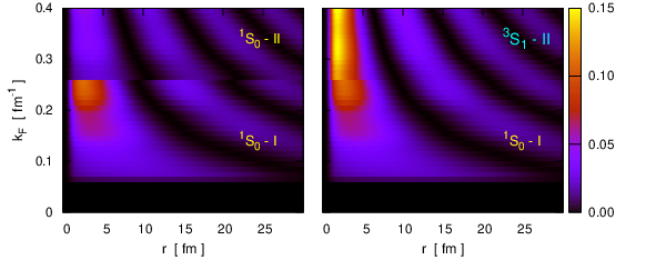
In fig. 10 we plot radial probability densities, , for S-wave bound states as functions of the relative distance . These solutions correspond to fm-1, Fermi momentum where the domains of phases I and II overlap. Panels (a) shows results for the channel in phase I (solid curve) and phase II (dashed curve). The same notation is used in panel (c) for the channel, where we also include the S-wave deuteron in free space (). Panel (b) displays and bound-state waves in phase I and II, respectively.

We observe that both and probability densities represent confined systems, exhibiting the same oscillatory behavior of Cooper pair solutions reported in refs. [28, 29]. In the case of the bound state shown in panel (a) we notice an outward shift of phase II solution relative to that in phase I. This indicates an enlargement of pairs in phase II relative to those in phase I, to be discussed later. The same feature is observed for deuterons in panel (c), where the free-space solution (solid black curve) is included. In this case we observe a similarity between the probability density of deuterons in free space with that of pairs in phase I. This suggests that deuterons maintain their size as long as they remain in phase I. These spatial aspects of in-medium dinucleon solutions shall further be discussed in the following section.
In fig. 11 we show contour plots for S-wave radial probabilities as functions of the relative distance and Fermi momentum . The left hand-side panel shows the solutions in phase I, with fm-1, together with those in phase II for fm-1. In the right hand-side panel the solution in phase II has been replaced by the corresponding solution. It is interesting to note how the two solutions appear in phase near the boundary fm-1.
4.2.3 Spatial properties
Cooper-like wavefunctions appear to have unique spatial properties, especially regarding their large size relative to the mean internucleon distance in the nuclear medium. This feature is already suggested in figs. 10 and 11, where the bound state wavefunctions are observed to decay slowly. Actually, these wavefunctions behave as for large radii, feature which poses convergence difficulties in the actual evaluation of mean radii or root-mean-square (rms) radii . In momentum space, in turn, we cannot make straightforward use of the customary identity [30] for the mean-square-radius
due to the discontinuity of the wavefunction at the Fermi surface. Actually, the above identity is valid as long as the wavefunction is bound in coordinate space, while in momentum space derivatives are continuous at all momenta. Such is not the case for , exhibiting a cut-off below , as a result of the sharpness of the sp momentum distribution. This cut off occurs at for pairs with no translational motion ().
To overcome the convergence difficulties posed in coordinate space evaluations, we propose to consider the Laplace transform of the density . This transform reads
| (31) |
Clearly, , the volume integral of the density. The small- behavior yields
from which we construct the alternative function given by
| (32) |
Since is finite, becomes always defined due to the exponential in the integrand. Thus, from an analysis of at small we can extract the mean radii and the mean-square-radii . A linear regression of eq. (32) for provides us with accurate fits, with correlations equal to unity out to six significant figures.
In fig. 12 we show results for the calculated mean radii and rms radii as functions of the Fermi momentum . Solutions for states , and are labeled as (1), (2) and (3), respectively. Empty and filled symbols denote results for phases I and II, respectively. Upper panels show (a) and (b) in fm units. Lower panels show results for the ratios (c) and (d), with , the mean internucleon separation at density . We note that both mean radii and rms radii for pairs (1) are larger than those for deuterons (2 and 3). What is also evident is that S-wave bound states experience a sudden increase of size in the transit from phase I to phase II. The rate of the change is more pronounced for deuterons than for pairs. Additionally, observing panels (c) and (d) we note that deuteron bound states in phase I are much smaller than the internucleon separation , while in phase II they remain bound with sizes several times the internucleon separation.

Another feature worth noting from panel (a) is that the size of deuterons in phase I remain roughly constant as a function of the density ( fm-1), with sizes similar to that in free space. In phase II, instead, they become fairly large objects with mean radii above 30 fm. In this respect deuterons change from very compact bosons in phase I to very extended ones in phase II. This is in contrast to pairs, where their sizes outpass the internucleon separation in both phases.
4.3 BCS pairing
The occurrence of dinucleon bound states in nuclear medium is closely related with nuclear pairing phenomena, mechanism responsible for the formation of Cooper pairs and emergence of superfluid and superconducting states of matter [1, 2]. Hence, it is of interest to explore some immediate implications of phases I and II for the sp potentials in the context of pairing gap equations. To this end we have solved the Bardeen-Cooper-Schrieffer (BCS) gap equations at zero temperature. These gap equations in triplet coupled states lead to coupled equations displaying an explicit angular dependence of the kernel, problem which has been addressed in ref. [31] in the context of pure neutron matter. However, an important simplification to the problem is obtained when the anisotropic kernel is angle averaged [32, 33]. Within this approximation the gap functions for states of orbital angular momentum take the form
| (33) |
where the quasiparticle energy reads
| (34) | ||||
| (35) |
Here is the chemical potential and , corresponds to the BHF sp spectrum. In this case solutions I and II for are treated independently, an issue that needs to be reexamined in more realistic calculations. The matrix elements of the bare interaction in a channel of total spin and isospin are given by
| (36) |
The corresponding normal () and anomalous () density distributions are given by
| (37) |
respectively. Self-consistency for the chemical potential is imposed through
| (38) |
with the nucleon density.
We have developed computer codes to solve BCS gap equations [eqs. (33-38)] following the method introduced by Baldo et al. [34]. The approach relies on the introduction of a reduced interaction which disconnects the low and high momentum components of the interaction but reproduces exactly the gap function in the low momentum regime.
In fig. 13 we show results for pairing gaps , in symmetric nuclear matter for and states. Empty and filled circles denote the use of BHF potentials in phase I and II, respectively. The inset shows the corresponding chemical potentials at low densities. Gap calculations in the overlapping domain of phases I and II have been performed in a simplified way, namely, pairing in phase I do not take into account phase II and vice versa. This simplification is intended to illustrate the most immediate consequences of the coexisting sp solutions.

Overall we observe that pairing gaps as function of the Fermi momentum, when fm-1, behave similarly to those published elsewhere [1]. The state in symmetric nuclear matter yields non-vanishing pairing gap up to , with a peak MeV, at . Similarly, pairing in the channel occurs up to , with a peak MeV, at . For fm-1, however, the coexisting phases for the sp potentials yield different energy gaps. These features contrast with the continuous low-density solutions for symmetric nuclear matter based on Gogny’s interaction [29]. It is also worth noting the correspondence between the Fermi momenta at which BCS pairing disappears and those where dinucleons in normal state within BHF get dissolved [panel (b) of fig. (9)]. What also becomes clear is that the maximum pairing gap in the channel is about 1/3 that in the state. Considering that the gap is given [33] by , this results in the actual suppression of pairing in symmetric nuclear matter when the coupled –gap equations are solved. From now on we shall only consider pairing in the channel.
Regarding the low density behavior of the chemical potential shown in the inset of fig. 13, we note that for the deuteron channel MeV, close to half the binding energy of the deuteron in free space. This is an expected result as it is well known that gap equations at low densities reduce to the Schrödinger equation in free space, where the anomalous density distribution takes the place of the wavefunction.
In BCS theory the coherence length sets a length scale for the distance between the two constituents forming Cooper pairs. In terms of the anomalous density distribution, this is obtained from
The evaluation of follows the procedure introduced in the previous section based on Laplace transforms, this time using the anomalous density. In fig. 14 we plot the coherence length as function of for the channel. The solid curve represents the internucleon separation . Note that the coherence length in phase I amounts between 0.4 and 0.6 times that in phase II. Therefore Cooper pairs in phase I are more compact than those in phase II, in correspondence with dinucleon radii. Additionally, in phase II outpasses the internucleon separation at fm-1, indicating that Cooper pairs extend beyond the mean separation between nucleons. Conversely, at low densities these objects become compact in the sense that their size is significantly smaller than the internucleon separation.

In fig. 15 we show a surface plot of the anomalous probability density calculated from the anomalous density distribution, as functions of the relative distance and Fermi momentum . These wavefunctions have been calculated using the sp potentials in phases I and II. We observe how the wavefunction spreads over greater extent of space as density increases, consistent with the behavior of the correlation length shown in fig. 14. Additionally, the Fermi momenta at which these functions peak appear in correspondence with the pairing gaps shown in fig. 13.

Having solved gap equations for phases I and II separately, we can now evaluate the condensate fraction in the channel. In terms of the normal and anomalous density distributions the condensate fraction of paired nucleons is given by [35]
| (39) |
In fig. 16 we plot the deuteron condensate fraction as a function of the Fermi momentum. We observe nearly total deuteron condensate (above 90%) at low densities, in phase I, accounting for Bose-Einstein condensation. The condensate fraction in phase II decreases monotonically from at , vanishing at fm-1.

4.4 Superfluidity
As mentioned earlier, the results discussed above help us to visualize the trend of nuclear pairing when each phase is considered separately. Additionally, the sp energies have been obtained within the BHF framework in normal state. The inclusion of superfluidity alters the momentum distribution and subsequently the sp fields [33], leaving open the issue on coexistence of the two phases found for the normal system. A consistent treatment of the problem would require considerably more efforts. Nonetheless, it is possible at the lowest order to estimate some immediate implications of superfluidity on the system along the line discussed in ref. [33].
In fig. 17 we plot the normal density at various as function of the ratio . Phase-I results (dashed curves) are shown up to fm-1, in steps of 0.02 fm-1. Phase-II results are shown from up to 1.8 fm-1 in steps of 0.1 fm-1. Note that the momentum distribution at high resembles very closely that of a normal Fermi distribution, consistent with the suppression of BCS pairing. As the density diminishes the momentum distribution spreads over and gets depleted below , in correspondence with the onset of superfluidity. This feature gets more pronounced in phase I.

To gauge the implications in the change of the momentum distribution when pairing is included, we have evaluated the energy per nucleon of the system including the condensation energy [33, 36], namely
| (40) |
The term from this expression which contains the sp fields is denoted as ,
| (41) |
whereas the last term represents the condensation energy and is denoted by ,
| (42) |
For the evaluation of above we use as obtained from eq. (37) based on sp energies in phase I and II, while the sp potential corresponds to that of normal BHF. Therefore it is not self-consistent in the sense that the evaluation of the sp potentials, , does not take into account the modification of the sp momentum distribution.
In fig. 18 we present the calculated as obtained from normal BHF (solid curves) and that using eq. (40), labeled ‘BHF+BCS’. The inset shows a close-up at low densities, where the solutions from the two phases are displayed. Circles denote the condensation energy () and squares the BHF mean field contribution (). Note that the condensate energy is weak at high densities but increases considerably at low densities, becoming the dominant (attractive) contribution in . The inclusion of pairing in phase I yields MeV, as observed from the inset (dashed curve in phase I). This feature is consistent with the fact that nearly total condensation occurs at low densities. What is also interesting to note is that the condensation energy intercepts at fm-1, about the same Fermi momentum at which the correlation length outpasses the mean internucleon separation (see fig. 14). Another result which emerges when pairing correlations are included is a slight decrease of the saturation density, up to about fm-1, without altering the saturation energy.

From the results discussed above it becomes clear that the disentanglement of BHF and superfluidity energies is meaningful at normal densities, i.e. near saturation, in contrast to low densities where the condensation energy amounts to a significant contribution to the total energy. This result leaves open the question on whether coexisting solutions persist if a more complete treatment of superfluidity is made.
5 Summary and outlook
Within the BHF approximation in BBG theory for symmetric nuclear matter at zero temperature, we have investigated the role of dinucleon structures over a wide range of densities (), with emphasis placed on the low-density regime. To this end we have calculated self-consistent sp potentials at Fermi momenta up to 1.75 fm-1 using the continuous choice, restricting the system to normal state. The study is based on the Argonne bare NN potential considering all partial waves up to , without three-body forces. The actual momentum dependence of the sp potential resulting from the evaluation of the mass operator has been retained. An explicit treatment was given to the occurrence of dinucleon bound states in the and channels during the evaluation of the mass operator.
As a result, two distinct families of solutions for the sp self-consistent potentials have been disclosed. The first class, , defines a surface in the plane at Fermi momenta below fm-1. The second class, , defines a surface at Fermi momenta above fm-1. In the range both solutions satisfy the self-consistency requirement, representing coexisting solutions. Solution I behaves as a correlated FG with slight repulsion relative to its non-interacting counterpart. Solution II represents a cohesive system up to the saturation point at fm-1, where we obtain MeV for its binding energy per nucleon. Each solution leads to distinct behaviors in their corresponding effective masses. While the correlated gas phase shows an increasing effective mass, reaching near , the condensed phase starts out with near-bare-mass sp at , reaching a maximum of at fm-1, and decreasing to about at saturation density. The emergence of massive sp solutions is a peculiarity of our results, in formal resemblance to Heavy Fermions (electrons) observed in unconventional superconductors [37, 38]. Work in progress using alternative realistic NN interactions also yields coexisting solutions with large effective masses, confirming the robustness of these findings.
Dinucleon structures associated with phases I and II for the sp fields exhibit unconventional spatial properties, with mean radii as large as fm. In the case of pairs, their size is always greater than the internucleon separation, with a sudden increase in the transit from phase I to phase II. Deuterons wavefunctions, in turn, appear very confined in phase I but outrange the internucleon separation in phase II.
Findings for nuclear matter in normal state were contrasted with those obtained from BCS pairing states, where BCS gap equations were solved considering sp spectra for phases I and II, independently. Nearly total deuteron condensate is obtained in phase I, decreasing monotonically in phase II up to fm-1, where pairing vanishes. The account for superfluidity lowers, by about 6%, the saturation density of nuclear matter relative to that obtained for normal state. At these densities the condensation energy is much weaker than the sp energy, below 30% for fm-1, justifying the separation between both contributions. Such is no longer the case at low densities where condensation and sp energies become comparable.
The disclosure of coexisting solutions in symmetric nuclear matter at low densities constitutes a major finding in this work. A crucial role was played by the explicit handling of dinucleon bound states together with refined methods to obtain self-consistent solutions for the sp fields. We have shown that the low-density solutions for the sp potentials are not quadratic in as they exhibit a sudden change of slope at . This feature rules out the reliability of using the effective mass approximation for the sp fields at low densities. In any case, the results reported here demonstrate that self-consistency within the BHF approximation, accounting for dinucleon bound states, is feasible without the need to assume a functional form to the sp fields.
We have next extended the present BHF study to include BCS pairing to lowest order in the sp momentum distribution. From this extension it becomes clear that the separation between BHF and superfluidity energies at low densities is not meaningfull. This leaves open the question as to whether the two coexisting solutions obtained at the BHF level persist if a more complete treatment of superfluidity were made. Actually, we have found that the inclusion of superfluidity attenuates considerably differences of the binding energy of the system in the coexisting range. In this regard, the inclusion of hole-hole propagation needs to be addressed to clarify whether coexisting phases correspond to actual physical properties of nuclear matter at low densities, or they are a result of an oversimplified description. The -matrix approximation in self-consistent Green’s function method [19, 6] offers a more coherent framework to reassess these issues.
The study presented here, where emphasis has been placed on pp correlations with explicit treatment of dinucleon bound states, is basic in the sense that multi-particle and clustering were not taken into account, although they are known be important in low-density clustering models [26, 39, 40]. Additionally, three-body forces are known to be crucial to account for the saturation point of nuclear matter [41], so that their effect at normal as well as high densities are expected to be important. However, beyond such simplifying assumptions as embodied by the BHF framework to treat nuclear correlations, it is reasonable to conceive that the model retains leading-order features in diluted nuclear environments expected to linger at low temperatures and isospin asymmetry. In this sense the findings reported in this work may provide additional conceptual tools to better understand the physics of diluted nuclear matter in the context of surface-sensitive nuclear reactions, the coupling to continuum in modeling nuclear open quantum systems [42] or dense star environments. From a more general perspective, it is also reasonable to expect that phase-coexistence in homogeneous nuclear matter in normal state breaks down as temperature and isospin asymmetry reach some critical values. Identifying the conditions under which coexistence persists constitute additional extension of this work.
Acknowledgements.
H.F.A. thanks colleagues at CEA, Bruyères-le-Châtel, France, for their warm hospitality during his stay where part of this work took place. The authors are indebted to M. Baldo and P. Schuck for useful discussions. Funding from CEA/DAM/DIF is acknowledged. This research has been funded in part by FONDECYT under grant No 1120396.Appendix A Integral equation with multiple roots on the real axis
A common technique to solve integral equations in momentum space is by discretizing the momentum in the range , reducing the problem to a matrix form. Thus, the equation
is reduced to the matrix equation
| (A.1) |
Here we are assuming that there are solutions to , with above the minimum value allowed by Pauli blocking, leading to the set of roots . The first sum in Eq. (A.1) represents the principal-value integral, for which we apply Gaussian-Legendre quadrature to integrate between consecutive roots, up to infinity.
Appendix B Adaptive trapezoidal quadrature
Consider the evaluation of the integral
| (B.1) |
with any finite function in the range . This function may also have a finite number of narrow peaks. Let us define
| (B.2) |
Additionally, let us consider the following sequence of sets of points in the interval : , , , etc. Note that the union of the first sets yields a uniform distribution of points, with no repetition of its elements. If the elements of the union are sequenced in ascending order, the separation between consecutive elements is . With this construction it can be verified that a trapezoidal quadrature can be represented by the recurrence
| (B.3) |
where is given by Eq. (B.2). In actual evaluations the iteration is interrupted at some when a convergence criteria for is met. If narrow peaks occur, the minimum should be such that becomes smaller than the smallest width. The advantage of this method is that the historical reckoning of is not discarded if a narrower mesh is needed. This is an important consideration whenever a single evaluation of is time-consuming.
Appendix C Evaluation of for S and D waves
Let us define
| (C.1) |
Denoting , and , the Fourier transform for for S waves becomes
| (C.2) |
The asymptotic behavior is identified for , case in which we get
| (C.3) |
In the case of D-waves we obtain
| (C.4) |
This result yields for large distances ()
References
- (1) R.A. Broglia, V. Zelevinsky, eds., Fifty Years of Nuclear BCS (World Scientific, Singapore, 2013).
- (2) A. Sedrakian, J.W. Clark, M. Alford, eds., Pairing in Fermionic Systems (World Scientific, Singapore, 2006).
- (3) Z.H. Li, U. Lombardo, H.J. Schulze, W. Zuo, L.W. Chen, H.R. Ma, Phys. Rev. C 74, 047304 (2006).
- (4) P. Gögelein, E.N.E. van Dalen, K. Gad, K.S.A. Hassaneen, H. Müther, Phys. Rev. C 79, 024308 (2009).
- (5) W.H. Dickhoff, D. Van Neck, Many-Body Theory Exposed! (World Scientific, Singapore, 2008).
- (6) H. Müther, W. Dickhoff, Phys. Rev. C 72, 054313 (2005).
- (7) A. Ramos, A. Polls, W. Dickhoff, Nuclear Physics A 503, 1 (1989).
- (8) M. Baldo, ed., Nuclear Methods and the Nuclear Equation of State, Vol. 8 of International Review of Nuclear Physics (World Scientific, Singapore, 1999).
- (9) H.Q. Song, M. Baldo, G. Giansiracusa, U. Lombardo, Phys. Rev. Lett. 81, 1584 (1998).
- (10) A. Lejeune, C. Mahaux, Nucl. Phys. A 295, 189 (1978).
- (11) J. Hüfner, C. Mahaux, Ann. Phys. 73, 525 (1972).
- (12) R. Sartor, Phys. Rev. C 27, 899 (1983).
- (13) M. Baldo, A. Fiasconaro, Phys. Lett. B 491, 240 (2000).
- (14) F.J. Aguayo, H.F. Arellano, Phys. Rev. C 78, 014608 (2008).
- (15) H.F. Arellano, J.P. Delaroche, Phys. Rev. C 83, 044306 (2011).
- (16) M.I. Haftel, F. Tabakin, Nuclear Physics A 158, 1 (1970).
- (17) H.F. Arellano, F.A. Brieva, W.G. Love, Phys. Rev. C 50, 2480 (1994).
- (18) R.B. Wiringa, V.G.J. Stoks, R. Schiavilla, Phys. Rev. C 51, 38 (1995).
- (19) P. Bożek, P. Czerski, Phys. Rev. C 66, 027301 (2002).
- (20) M. Baldo, C. Maieron, P. Schuck, X. Viñas, Nuclear Physics A 736, 241 (2004).
- (21) H.V. von Geramb, The Interaction Between Medium Energy Nucleons in Nuclei (American Institute of Physics, New York, 1983).
- (22) K. Amos, P.J. Dortmans, H.V. von Geramb, S. Karataglidis, J. Raynal, Advances in Nuclear Physics, Vol. 25 of Advances in Nuclear Physics (Springer, New York, 2000).
- (23) T.H. Phat, N.T. Anh, D.T. Tam, Phys. Rev. C 84, 024321 (2011).
- (24) B. Vonderfecht, C. Gearhart, W. Dickhoff, A. Polls, A. Ramos, Phys. Lett. B 253, 1 (1991).
- (25) L.N. Cooper, Phys. Rev. 104, 1189 (1956).
- (26) S. Typel, G. Röpke, T. Klähn, D. Blaschke, H.H. Wolter, Phys. Rev. C 81, 015803 (2010).
- (27) G. Röpke, Phys. Rev. C 79, 014002 (2009).
- (28) M. Baldo, U. Lombardo, P. Schuck, Phys. Rev. C 52, 975 (1995).
- (29) M. Matsuo, Phys. Rev. C 73, 044309 (2006).
- (30) B.Y. Sun, H. Toki, J. Meng, Phys. Lett. B 683, 134 (2010).
- (31) T. Tatsuyuki, R. Tamagaki, Prog. Theor. Phys. Supplement 112, 27 (1993).
- (32) D.J. Dean, M. Hjorth-Jensen, Rev. Mod. Phys. 75, 607 (2003).
- (33) U. Lombardo, H.J. Schulze, W. Zuo, Phys. Rev. C 59, 2927 (1999).
- (34) M. Baldo, J. Cugnon, A. Lejeune, U. Lombardo, Nuclear Physics A 515, 409 (1990).
- (35) L. Salasnich, Phys. Rev. C 84, 067301 (2011).
- (36) A.J. Fetter, J.D. Walecka, Quantum Theory of Many-Particle Systems (McGraw-Hill Book Company, New York, 1971).
- (37) G.R. Stewart, Rev. Mod. Phys. 56, 755 (1984).
- (38) P. Gegenwart, Q. Si, F. Steglich, Nature Physics 4, 186 (2008).
- (39) T. Sogo, G. Röpke, P. Schuck, Phys. Rev. C 82, 034322 (2010).
- (40) C. Horowitz, A. Schwenk, Nuclear Physics A 776, 55 (2006).
- (41) Z.H. Li, U. Lombardo, H.J. Schulze, W. Zuo, Phys. Rev. C 77, 034316 (2008).
- (42) N. Michel, W. Nazarewicz, J. Okolowicz, M. Ploszajczak, J. Phys. G: Nucl. Part. Phys. 37, 064042 (2010).