跳到论文正文
W Papers独立论文阅读器 arXiv:1410.7693 论文正文 计算阅读时间 · 0%
引用这篇论文根据当前论文元数据生成,正式投稿前建议核对。


License: arXiv.org perpetual non-exclusive license
arXiv:1410.7693v3 [math.CO] 25 Oct 2015

Domino tilings of three-dimensional regions:
flips and twists

Pedro H. Milet     Nicolau Saldanha
Abstract

In this paper, we consider domino tilings of regions of the form 𝒟×[0,n]\mathcal{D}\times[0,n], where 𝒟\mathcal{D} is a simply connected planar region and n∈ℕn\in{\mathbb{N}}. It turns out that, in nontrivial examples, the set of such tilings is not connected by flips, i.e., the local move performed by removing two adjacent dominoes and placing them back in another position. We define an algebraic invariant, the twist, which partially characterizes the connected components by flips of the space of tilings of such a region. Another local move, the trit, consists of removing three adjacent dominoes, no two of them parallel, and placing them back in the only other possible position: performing a trit alters the twist by ±1\pm 1. We give a simple combinatorial formula for the twist, as well as an interpretation via knot theory. We prove several results about the twist, such as the fact that it is an integer and that it has additive properties for suitable decompositions of a region.

1 Introduction

Tiling problems have received a lot of attention in the second half of the twentieth century, two-dimensional domino and lozenge tilings in particular. For instance, Kasteleyn [12], Conway [6], Thurston [23], Elkies, Propp et al. [11, 5, 7], Kenyon and Okounkov [14, 13] have come up with very interesting techniques, ranging from abstract algebra to probability. More relevant to the discussion in this paper are the problems of flip accessibility (e.g., [22]).

Attempts to generalize some of these techniques to the three-dimensional case were made. The problem of counting domino tilings, even of contractible regions, is known to be computationally hard (see [19]), but some asymptotic results, even for higher dimensions, date as far back as 1966 (see [10, 4, 8]). In a different direction, some “typically two-dimensional” properties were carried over to specific families of three-dimensional regions (see [20, 15, 3]).

Others have considered difficulties with connectivity by local moves in dimension higher than two (see, e.g., [20]). We propose an algebraic invariant that could help understand the structure of connected component by flips in dimension three.
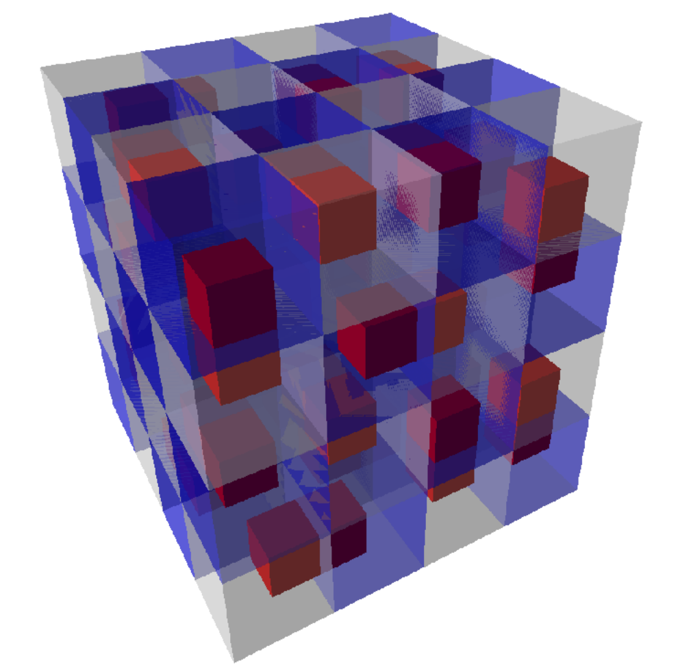
Refer to caption
Figure 1: A tiling of a 4×4×44\times 4\times 4 box.

In this paper, we investigate tilings of contractible regions by domino brick pieces, or dominoes, which are simply 2×1×12\times 1\times 1 rectangular cuboids. An example of such a tiling is shown in Figure 1. While this 3D representation of tilings may be attractive, it is also somewhat difficult to work with. Hence, we prefer to work with a 2D representation of tilings, which is shown in Figure 4.

A key element in our study is the concept of a flip, which is a straightforward generalization of the two-dimensional one. We perform a flip on a tiling by removing two (adjacent and parallel) domino bricks and placing them back in the only possible different position. The removed pieces form a 2×2×12\times 2\times 1 slab, in one of three possible directions (see Figure 4). The flip connected component of a tiling tt of a three-dimensional region ℛ\mathcal{R} is the set of all tilings of ℛ\mathcal{R} that can be reached from tt after a sequence of flips. It turns out that for large regions the number of flip connected components is also large, but some of them may contain many tilings. One of the aims of this paper is to study such connected components.

As in [18], we also consider the trit, which is a move that happens within a 2×2×22\times 2\times 2 cube with two opposite “holes”, and which has an orientation (positive or negative). More precisely, we remove three dominoes, no two of them parallel, and place them back in the only other possible configuration (see Figure 4).

x y ∈ z [ 0 , 1 ] ∈ z [ 1 , 2 ] ∈ z [ 2 , 3 ] ∈ z [ 3 , 4 ]
Figure 2: A tiling of the box ℬ=[0,4]×[0,4]×[0,4]\mathcal{B}=[0,4]\times[0,4]\times[0,4] box in our notation. The xx and yy axis are drawn, and zz points towards the paper, so that floors to the right have higher zz coordinates. Dominoes that are parallel to the xx or yy axis are represented as 2D dominoes, since they are contained in a single floor. Dominoes parallel to the zz axis are represented as circles, with the following convention: if the corresponding domino connects a floor with the floor to the left of it, the circle is painted red; otherwise, it is painted white. Thus, for example, in Figure 4, each of the four white circles on the leftmost floor represents the same domino as the red circles on the floor directly to the right of it. The squares highlighted in yellow represent cubes whose centers have the same xx and yy coordinates. Notice the top two yellow cubes are connected by a domino parallel to the zz axis, as well as the bottom two. The squares highlighted in green also represent cubes whose center have the same xx and yy coordinates, but the dominoes involving these cubes are not parallel to the zz axis.
Figure 3: All flips available in tiling (1). The 2×2×12\times 2\times 1 slabs involved in the flips taking (1) to (2), (3) and (4) are highlighted: they illustrate the three possible relative positions of dominoes in a flip.
Figure 4: An example of a negative trit. The affected cubes are highlighted in yellow.

A cylinder is a region of the form 𝒟×[0,n]\mathcal{D}\times[0,n] (possibly rotated), where 𝒟⊂ℝ2\mathcal{D}\subset{\mathbb{R}}^{2} is a simply connected planar region with connected interior. In this paper, we introduce an algebraic invariant, the twist Tw⁡(t)\operatorname{Tw}(t), defined in Section 3 for tilings of a cylinder.

In [18], we study cylinders with n=2n=2, called duplex regions. Although they are related to the general theory, tilings of these regions have some interesting characteristics of their own; in particular, we can define a polynomial Pt​(q)P_{t}(q) for tilings of duplex regions which is invariant by flips and which is finer than the twist. However, this construction breaks down when the duplex region is embedded in a region with more floors (see [18] for details).

Theorem 1.

Let ℛ\mathcal{R} be a cylinder, and tt a tiling of ℛ\mathcal{R}. The twist Tw⁡(t)\operatorname{Tw}(t) is an integer with the following properties:

  1. (i)

    If a tiling t1t_{1} is reached from t0t_{0} after a flip, then Tw⁡(t1)=Tw⁡(t0)\operatorname{Tw}(t_{1})=\operatorname{Tw}(t_{0}).

  2. (ii)

    If a tiling t1t_{1} is reached from t0t_{0} after a single positive trit, then Tw⁡(t1)−Tw⁡(t0)=1\operatorname{Tw}(t_{1})-\operatorname{Tw}(t_{0})=1.

  3. (iii)

    If ℛ\mathcal{R} is a duplex region, then Tw⁡(t)=Pt′​(1)\operatorname{Tw}(t)=P_{t}^{\prime}(1) for any tiling tt of ℛ\mathcal{R}.

  4. (iv)

    Suppose a cylinder ℛ=⋃1≤i≤mℛi\mathcal{R}=\bigcup_{1\leq i\leq m}\mathcal{R}_{i}, where each ℛi\mathcal{R}_{i} is a cylinder (they need not have the same axis) and such that i≠j⇒int⁡(ℛi)∩int⁡(ℛj)≠∅i\neq j\Rightarrow\operatorname{int}(\mathcal{R}_{i})\cap\operatorname{int}(\mathcal{R}_{j})\neq\emptyset. Then there exists a constant K∈ℤK\in{\mathbb{Z}} such that, for any family (ti)1≤i≤n(t_{i})_{1\leq i\leq n}, tit_{i} a tiling of ℛi\mathcal{R}_{i},

    Tw⁡(⨆1≤i≤mti)=K+∑1≤i≤mTw⁡(ti).\operatorname{Tw}\left(\bigsqcup_{1\leq i\leq m}t_{i}\right)=K+\sum_{1\leq i\leq m}\operatorname{Tw}(t_{i}).

The definitions of twist are somewhat technical and involve a relatively lengthy discussion. We shall give two different but equivalent definitions: the first one, given in Section 3, is a sum over pairs of dominoes. At first sight, this formula gives a number in 14​ℤ\frac{1}{4}{\mathbb{Z}} and depends on a choice of axis. However, it turns out that, for cylinders, this number is an integer, and different choices of axis yield the same result. The proof of this claim will be completed in Section 6, and it relies on the second definition, which uses the concepts of writhe and linking number from knot theory (see, e.g., [1]).

One can ask whether the twist can be extended to a broader class of regions. The following (see [16]) holds: let ℛ\mathcal{R} be a simply connected region (not necessarily a cylinder), t0t_{0} and t1t_{1} be two tilings of ℛ\mathcal{R}. Suppose ℬ⊃ℛ\mathcal{B}\supset\mathcal{R} is a box and t∗t_{*} is a tiling of ℬ∖ℛ\mathcal{B}\setminus\mathcal{R} (it is not true for arbitrary regions ℛ\mathcal{R} that ℬ\mathcal{B} and t∗t_{*} exist). Define TW⁡(t0,t1)=Tw⁡(t0⊔t∗)−Tw⁡(t1⊔t∗)\operatorname{TW}(t_{0},t_{1})=\operatorname{Tw}(t_{0}\sqcup t_{*})-\operatorname{Tw}(t_{1}\sqcup t_{*}): this turns out to depend neither on the choice of box ℬ\mathcal{B} nor on the choice of tiling t∗t_{*}. Therefore, if we choose a base tiling t0t_{0} and define Tw⁡(t)=TW⁡(t,t0)\operatorname{Tw}(t)=\operatorname{TW}(t,t_{0}), then Tw⁡(t)\operatorname{Tw}(t) satisfies items (i) and (ii) in Theorem 1. Different choices of base tiling only alter the twist by an additive constant.

In addition to the combinatorial and knot-theoretic interpretations developed in this article, it is also possible to give homological interpretations for the twist. These homological constructions are reminiscent of the two-dimensional height functions (see [23]), although they behave more like “height forms”. The concept of flux (or flow), as in [22] and [21], also becomes relevant. Although we will not discuss these constructions here, this homological point of view inspired many of our definitions.

One might also ask what the possible values for the twist of a certain region are. Some results in this direction are proved in [16]: for instance, it turns out that, for a box of dimensions L×M×NL\times M\times N with L≥M≥NL\geq M\geq N (and L​M​NLMN even), the maximum possible value for the twist is of the order of L​M​N2LMN^{2}.

The present paper is structured in the following manner: Section 2 introduces some basic definitions and notations that will be used throughout the paper. In Section 3, we define the invariant for cylinders, and prove its most basic properties. In Sections 4, 5, 6 and 7, we present different aspects of a connection between the twist of tilings and a few classical concepts from knot theory. Section 4 contains the “topological groundwork”, which consists of a number of definitions and results that help establish topological interpretations of the twist, and which are extensively used in the sections that follow it. In Section 5, we introduce a different formula for the twist of cylinders, and show that this new formula allows us to prove (once again, via topology) that the twist must always be an integer. In Section 6, we prove that the value of the twist of cylinders does not depend on the choice of axis, which is one of the main results in the paper. In Section 7, we discuss additive properties of the twist, and prove item (iv) in Theorem 1. Finally, Section 8 contains some examples and counterexamples that help illustrate the theory.

This paper closely corresponds to part of the first author’s PhD thesis [16]; the authors thank the examination board for helpful comments and suggestions. The authors are also thankful for the generous support of CNPq, CAPES and FAPERJ (Brazil).

2 Definitions and Notation

This section contains general notations and conventions that are used throughout the article, although definitions that involve a lengthy discussion or are intrinsic of a given section might be postponed to another section.

If nn is an integer, n♯{n}^{\sharp} will denote n+12n+{\frac{1}{2}} (in music theory, D​♯D\sharp is a half tone higher than DD in pitch). We also define ℤ♯{{\mathbb{Z}}}^{\sharp} to be the set {n♯|n∈ℤ}\{{n}^{\sharp}|n\in{\mathbb{Z}}\}.

Given v→1,v→2,v→3∈ℝ3\vec{v}_{1},\vec{v}_{2},\vec{v}_{3}\in{\mathbb{R}}^{3}, det(v→1,v→2,v→3)=v→1⋅(v→2×v→3)\det(\vec{v}_{1},\vec{v}_{2},\vec{v}_{3})=\vec{v}_{1}\cdot(\vec{v}_{2}\times\vec{v}_{3}) denotes the determinant of the 3×3×33\times 3\times 3 matrix whose ii-th line is v→i\vec{v}_{i}, i=1,2,3i=1,2,3. If β=(β→1,β→2,β→3)\beta=(\vec{\beta}_{1},\vec{\beta}_{2},\vec{\beta}_{3}) is a basis, write det(β)=det(β→1,β→2,β→3)\det(\beta)=\det(\vec{\beta}_{1},\vec{\beta}_{2},\vec{\beta}_{3}).

We denote the three canonical basis vectors as 𝐢→=(1,0,0)\vec{\mathbf{i}}=(1,0,0), 𝐣→=(0,1,0)\vec{\mathbf{j}}=(0,1,0) and 𝐤→=(0,0,1).\vec{\mathbf{k}}=(0,0,1). We denote by Δ={𝐢→,𝐣→,𝐤→}\Delta=\{\vec{\mathbf{i}},\vec{\mathbf{j}},\vec{\mathbf{k}}\} the set of canonical basis vectors, and Φ={±𝐢→,±𝐣→,±𝐤→}\Phi=\{\pm\vec{\mathbf{i}},\pm\vec{\mathbf{j}},\pm\vec{\mathbf{k}}\}. Let 𝐁={β=(β→1,β→2,β→3)|β→i∈Φ,det(β)=1}\mathbf{B}=\{\beta=(\vec{\beta}_{1},\vec{\beta}_{2},\vec{\beta}_{3})|\vec{\beta}_{i}\in\Phi,\det(\beta)=1\} be the set of positively oriented bases with vectors in Φ\Phi.

A basic cube is a closed unit cube in ℝ3{\mathbb{R}}^{3} whose vertices lie in ℤ3{\mathbb{Z}}^{3}. For (x,y,z)∈ℤ3(x,y,z)\in{\mathbb{Z}}^{3}, the notation C⁡(x♯,y♯,z♯)C\left({x}^{\sharp},{y}^{\sharp},{z}^{\sharp}\right) denotes the basic cube (x,y,z)+[0,1]3(x,y,z)+[0,1]^{3}, i.e., the closed unit cube whose center is (x♯,y♯,z♯)\left({x}^{\sharp},{y}^{\sharp},{z}^{\sharp}\right); it is white (resp. black) if x+y+zx+y+z is even (resp. odd). If C=C⁡(x♯,y♯,z♯)C=C\left({x}^{\sharp},{y}^{\sharp},{z}^{\sharp}\right), define color⁡(C)=(−1)x+y+z+1\operatorname{color}(C)=(-1)^{x+y+z+1}, or, in other words, 11 if CC is black and −1-1 if CC is white. A region is a finite union of basic cubes. A domino brick or domino is the union of two basic cubes that share a face. A tiling of a region is a covering of this region by dominoes with pairwise disjoint interiors.

We sometimes need to refer to planar objects. Let π\pi denote either ℝ2{\mathbb{R}}^{2} or a basic plane contained in ℝ3{\mathbb{R}}^{3}, i.e., a plane with equation x=kx=k, y=ky=k or z=kz=k for some k∈ℤk\in{\mathbb{Z}}. A basic square in π\pi is a unit square Q⊂πQ\subset\pi with vertices in ℤ2{\mathbb{Z}}^{2} (if π=ℝ2\pi={\mathbb{R}}^{2}) or ℤ3{\mathbb{Z}}^{3}. A planar region D⊂πD\subset\pi is a finite union of basic squares.

A region ℛ\mathcal{R} is a cubiculated cylinder or multiplex region if there exist a basic plane π\pi with normal vector v→∈Δ\vec{v}\in\Delta, a simply connected planar region 𝒟⊂π\mathcal{D}\subset\pi with connected interior and a positive integer nn such that

ℛ=𝒟+[0,n]v→={p+sv→|p∈𝒟,s∈[0,n]};\mathcal{R}=\mathcal{D}+[0,n]\vec{v}=\{p+s\vec{v}|p\in\mathcal{D},s\in[0,n]\};

we usually call ℛ\mathcal{R} a cylinder for brevity. The cylinder ℛ\mathcal{R} above has base 𝒟\mathcal{D}, axis v→\vec{v} and depth nn. For instance, a cylinder with axis 𝐤→\vec{\mathbf{k}} and depth nn can be written as 𝒟×[k,k+n]\mathcal{D}\times[k,k+n], where 𝒟⊂ℝ2\mathcal{D}\subset{\mathbb{R}}^{2}. A v→\vec{v}-cylinder means a cylinder with axis v→\vec{v}. A duplex region (see [18]) is a cylinder with depth 22.

We sometimes want to point out that the hypothesis of simple connectivity (of a cylinder) is not being used: therefore, a pseudocylinder with base 𝒟\mathcal{D}, axis v→\vec{v} and depth nn has the same definition as above, except that the planar region 𝒟⊂π\mathcal{D}\subset\pi is only assumed to have connected interior (and is not necessarily simply connected).

A box is a region of the form ℬ=[L0,L1]×[M0,M1]×[N0,N1]\mathcal{B}=[L_{0},L_{1}]\times[M_{0},M_{1}]\times[N_{0},N_{1}], where Li,Mi,Ni∈ℤL_{i},M_{i},N_{i}\in{\mathbb{Z}}. Boxes are special cylinders, in the sense that we can take any vector v→∈Δ\vec{v}\in\Delta as the axis. In fact, boxes are the only regions that satisfy the definition of cylinder for more than one axis.

Regarding notation, Figures 4, 4 and 4 were drawn with β=(𝐢→,𝐣→,𝐤→)\beta=(\vec{\mathbf{i}},\vec{\mathbf{j}},\vec{\mathbf{k}}) in mind. However, any β∈𝐁\beta\in\mathbf{B} allows for such representations, as follows: we draw β→3\vec{\beta}_{3} as perpendicular to the paper (pointing towards the paper). If π=β→3⟂\pi=\vec{\beta}_{3}^{\perp}, we then draw each floor ℛ∩(π+[n,n+1]​β→3)\mathcal{R}\cap(\pi+[n,n+1]\vec{\beta}_{3}) as if it were a plane region. Floors are drawn from left to right, in increasing order of nn.

The flip connected component of a tiling tt of a region ℛ\mathcal{R} is the set of all tilings of ℛ\mathcal{R} that can be reached from tt after a sequence of flips.

Suppose tt is a tiling of a region ℛ\mathcal{R}, and let ℬ=[l,l+2]×[m,m+2]×[n,n+2]\mathcal{B}=[l,l+2]\times[m,m+2]\times[n,n+2], with l,m,n∈ℕl,m,n\in{\mathbb{N}}. Suppose ℬ∩ℛ\mathcal{B}\cap\mathcal{R} contains exactly three dominoes of tt, no two of them parallel: notice that this intersection can contain six, seven or eight basic cubes of ℛ\mathcal{R}. Also, a rotation (it can even be a rotation, say, in the X​YXY plane), can take us either to the left drawing or to the right drawing in Figure 5.

Figure 5: The anatomy of a positive trit (from left to right). The trit that takes the right drawing to the left one is a negative trit. The squares with no dominoes represent basic cubes that may or may not be in ℛ\mathcal{R} (see Figure 4 for an example).

If we remove the three dominoes of tt contained in ℬ∩ℛ\mathcal{B}\cap\mathcal{R}, there is only one other possible way we can place them back. This defines a move that takes tt to a different tiling t′t^{\prime} by only changing dominoes in ℬ∩ℛ\mathcal{B}\cap\mathcal{R}: this move is called a trit. If the dominoes of tt contained in ℬ∩ℛ\mathcal{B}\cap\mathcal{R} are a plane rotation of the left drawing in Figure 5, then the trit is positive; otherwise, it’s negative. Notice that the sign of the trit is unaffected by translations (colors of cubes don’t matter) and rotations in ℝ3{\mathbb{R}}^{3} (provided that these transformations take ℤ3{\mathbb{Z}}^{3} to ℤ3{\mathbb{Z}}^{3}). A reflection, on the other hand, switches the sign (the drawing on the right can be obtained from the one on the left by a suitable reflection).

3 The twist for cylinders

For a domino dd, define v→​(d)∈Φ\vec{v}(d)\in\Phi to be the center of the black cube contained in dd minus the center of the white one. We sometimes draw v→​(d)\vec{v}(d) as an arrow pointing from the center of the white cube to the center of the black one.

For a set X⊂ℝ3X\subset{\mathbb{R}}^{3} and u→∈Φ\vec{u}\in\Phi, we define the (open) u→\vec{u}-shade of XX as

𝒮u→(X)=int((X+[0,∞)u→)∖X)=int({x+su→∈ℝ3|x∈X,s∈[0,∞)}∖X),\mathcal{S}^{\vec{u}}(X)=\operatorname{int}((X+[0,\infty)\vec{u})\setminus X)=\operatorname{int}\left(\{x+s\vec{u}\in{\mathbb{R}}^{3}|x\in X,s\in[0,\infty)\}\setminus X\right),

where int⁡(Y)\operatorname{int}(Y) denotes the interior of YY. The closed u→\vec{u}-shade 𝒮¯u→​(X)\bar{\mathcal{S}}^{\vec{u}}(X) is the closure of 𝒮u→​(X)\mathcal{S}^{\vec{u}}(X). We shall only refer to u→\vec{u}-shades of unions of basic cubes or basic squares, such as dominoes.

Figure 6: Tiling of a 4×4×44\times 4\times 4 box, with three distinguished dominoes (painted yellow, green and cyan), whose 𝐤→\vec{\mathbf{k}}-shades are highlighted in the same color as they are. Notice that the yellow shade intersects four dominoes, the green shade intersects three, and the cyan shade, only one.

Given two dominoes d0d_{0} and d1d_{1} of tt, we define the effect of d0d_{0} on d1d_{1} along u→\vec{u}, as:

τu→​(d0,d1)={14​det(v→​(d1),v→​(d0),u→),d1∩𝒮u→​(d0)≠∅0,otherwise\tau^{\vec{u}}(d_{0},d_{1})=\begin{cases}\frac{1}{4}\det(\vec{v}(d_{1}),\vec{v}(d_{0}),\vec{u}),&d_{1}\cap\mathcal{S}^{\vec{u}}(d_{0})\neq\emptyset\\ 0,&\mbox{otherwise}\end{cases}

In other words, τu→​(d0,d1)\tau^{\vec{u}}(d_{0},d_{1}) is zero unless the following three things happen: d1d_{1} intersects the u→\vec{u}-shade of d0d_{0}; neither d0d_{0} nor d1d_{1} are parallel to u→\vec{u}; and d0d_{0} is not parallel to d1d_{1}. When τu→​(d0,d1)\tau^{\vec{u}}(d_{0},d_{1}) is not zero, it’s either 1/41/4 or −1/4-1/4 depending on the orientations of v→​(d0)\vec{v}(d_{0}) and v→​(d1)\vec{v}(d_{1}).

For example, in Figure 6, for u→=𝐤→\vec{u}=\vec{\mathbf{k}}, the yellow domino dYd_{Y} has no effect on any other domino: τ𝐤→​(dY,d)=0\tau^{\vec{\mathbf{k}}}(d_{Y},d)=0 for every domino dd in the tiling. The green domino dGd_{G}, however, affects the two dominoes in the rightmost floor which intersect its 𝐤→\vec{\mathbf{k}}-shade, and τ𝐢→​(dG,d)=1/4\tau^{\vec{\mathbf{i}}}(d_{G},d)=1/4 for both these dominoes.

If tt is a tiling, we define the u→\vec{u}-pretwist as

Tu→​(t)=∑d0,d1∈tτu→​(d0,d1).T^{\vec{u}}(t)=\sum_{d_{0},d_{1}\in t}\tau^{\vec{u}}(d_{0},d_{1}).

For example, the tiling on the left of Figure 4 has 𝐤→\vec{\mathbf{k}}-pretwist equal to 11. To see this, notice that each of the four dominoes of the leftmost floor that are not parallel to 𝐤→\vec{\mathbf{k}} has nonzero effect along 𝐤→\vec{\mathbf{k}} on exactly one domino of the rightmost floor, and this effect is 1/41/4 in each case. The reader may also check that the 𝐤→\vec{\mathbf{k}}-pretwist of the tiling in Figure 6 is 00.

Lemma 3.1.

For any pair of dominoes d0d_{0} and d1d_{1} and any u→∈Φ\vec{u}\in\Phi, τu→​(d0,d1)=τ−u→​(d1,d0)\tau^{\vec{u}}(d_{0},d_{1})=\tau^{-\vec{u}}(d_{1},d_{0}). In particular, for a tiling tt of a region we have T−u→​(t)=Tu→​(t)T^{-\vec{u}}(t)=T^{\vec{u}}(t).

Proof.

Just notice that d1∩𝒮u→​(d0)≠∅d_{1}\cap\mathcal{S}^{\vec{u}}(d_{0})\neq\emptyset if and only if d0∩𝒮−u→​(d1)≠∅,d_{0}\cap\mathcal{S}^{-\vec{u}}(d_{1})\neq\emptyset, and det(v→​(d1),v→​(d0),u→)=det(v→​(d0),v→​(d1),−u→)\det(\vec{v}(d_{1}),\vec{v}(d_{0}),\vec{u})=\det(\vec{v}(d_{0}),\vec{v}(d_{1}),-\vec{u}). ∎

Translating both dominoes by a vector with integer coordinates clearly does not affect τu→​(d0,d1)\tau^{\vec{u}}(d_{0},d_{1}), as det(v→​(d1),v→​(d0),u→)=det(−v→​(d1),−v→​(d0),u→)\det(\vec{v}(d_{1}),\vec{v}(d_{0}),\vec{u})=\det(-\vec{v}(d_{1}),-\vec{v}(d_{0}),\vec{u}). Therefore, if tt is a tiling and f⁡(p)=p+bf(p)=p+b, where b∈ℤ3b\in{\mathbb{Z}}^{3}, then Tu→​(f⁡(t))=Tu→​(t)T^{\vec{u}}(f(t))=T^{\vec{u}}(t).

Lemma 3.2.

Let ℛ\mathcal{R} be a region, and let w→∈Δ\vec{w}\in\Delta. Consider the reflection r=rw→:ℝ3→ℝ3:p↦p−2​(p⋅w→)​w→r=r_{\vec{w}}:{\mathbb{R}}^{3}\to{\mathbb{R}}^{3}:p\mapsto p-2(p\cdot\vec{w})\vec{w}; notice that r⁡(ℛ)r(\mathcal{R}) is a region. If tt is a tiling of ℛ\mathcal{R} and u→∈Φ\vec{u}\in\Phi, then the tiling r⁡(t)={r⁡(d),d∈t}r(t)=\{r(d),d\in t\} of r⁡(ℛ)r(\mathcal{R}) satisfies Tu→​(r⁡(t))=−Tu→​(t)T^{\vec{u}}(r(t))=-T^{\vec{u}}(t).

Proof.

Given a domino dd of tt, notice that v→​(r⁡(d))=−r⁡(v→​(d))\vec{v}(r(d))=-r(\vec{v}(d)) and that 𝒮u→​(r⁡(d))=r⁡(𝒮r⁡(u→)​(d))\mathcal{S}^{\vec{u}}(r(d))=r(\mathcal{S}^{r(\vec{u})}(d)). Therefore, r⁡(d1)∩𝒮u→​(r⁡(d0))≠∅⇔d1∩Sr⁡(u→)​(d0)≠∅r(d_{1})\cap\mathcal{S}^{\vec{u}}(r(d_{0}))\neq\emptyset\Leftrightarrow d_{1}\cap S^{r(\vec{u})}(d_{0})\neq\emptyset and

det(v→​(r⁡(d1)),v→​(r⁡(d0)),u→)=det(−r⁡(v→​(d1)),−r⁡(v→​(d0)),u→)\displaystyle\det(\vec{v}(r(d_{1})),\vec{v}(r(d_{0})),\vec{u})=\det(-r(\vec{v}(d_{1})),-r(\vec{v}(d_{0})),\vec{u})
=det(r(v→(d1)),r(v→(d0)),r(r(u→)))=−det(v→(d1),v→(d0),r(u→)).\displaystyle=\det(r(\vec{v}(d_{1})),r(\vec{v}(d_{0})),r(r(\vec{u})))=-\det(\vec{v}(d_{1}),\vec{v}(d_{0}),r(\vec{u})).

Therefore, τu→​(r⁡(d0),r⁡(d1))=−τr⁡(u→)​(d0,d1)\tau^{\vec{u}}(r(d_{0}),r(d_{1}))=-\tau^{r(\vec{u})}(d_{0},d_{1}) and thus Tu→​(r⁡(t))=−Tr⁡(u→)​(t)T^{\vec{u}}(r(t))=-T^{r(\vec{u})}(t). Since r⁡(u→)=±u→r(\vec{u})=\pm\vec{u}, Lemma 3.1 implies that Tu→​(r⁡(t))=−Tu→​(t)T^{\vec{u}}(r(t))=-T^{\vec{u}}(t), completing the proof. ∎

A natural question at this point concerns how the choice of u→\vec{u} affects Tu→T^{\vec{u}}. It turns out that it will take us some preparation before we can tackle this question.

Proposition 3.3.

If ℛ\mathcal{R} is a cylinder and tt is a tiling of ℛ\mathcal{R},

T𝐢→​(t)=T𝐣→​(t)=T𝐤→​(t)∈ℤ.T^{\vec{\mathbf{i}}}(t)=T^{\vec{\mathbf{j}}}(t)=T^{\vec{\mathbf{k}}}(t)\in{\mathbb{Z}}.
Proof.

Follows directly from Propositions 6.4 and 6.10 below. ∎

This result doesn’t hold in pseudocylinders or in more general simply connected regions; see Section 8 for counterexamples.

Definition 3.4.

For a tiling tt of a cylinder ℛ\mathcal{R}, we define the twist Tw⁡(t)\operatorname{Tw}(t) as

Tw⁡(t)=T𝐢→​(t)=T𝐣→​(t)=T𝐤→​(t).\operatorname{Tw}(t)=T^{\vec{\mathbf{i}}}(t)=T^{\vec{\mathbf{j}}}(t)=T^{\vec{\mathbf{k}}}(t).

Until Section 6, we will not use Proposition 3.3, and will only refer to pretwists.

Let u→∈Δ\vec{u}\in\Delta, and let β=(β→1,β→2,β→3)∈𝐁\beta=(\vec{\beta}_{1},\vec{\beta}_{2},\vec{\beta}_{3})\in\mathbf{B} be such that β→3=u→\vec{\beta}_{3}=\vec{u}. A region ℛ\mathcal{R} is said to be fully balanced with respect to u→\vec{u} if for each square Q=p+[0,2]​β→1+[0,2]​β→2Q=p+[0,2]\vec{\beta}_{1}+[0,2]\vec{\beta}_{2}, where p∈ℤ3p\in{\mathbb{Z}}^{3} and Q⊂ℛQ\subset\mathcal{R}, each of the two sets 𝒜u→=ℛ∩𝒮¯u→​(Q)\mathcal{A}^{\vec{u}}=\mathcal{R}\cap\bar{\mathcal{S}}^{\vec{u}}(Q) and 𝒜−u→=ℛ∩𝒮¯−u→​(Q)\mathcal{A}^{-\vec{u}}=\mathcal{R}\cap\bar{\mathcal{S}}^{-\vec{u}}(Q) contains as many black cubes as white ones. In other words,

∑C⊂𝒜u→color⁡(C)=∑C⊂𝒜−u→color⁡(C)=0.\sum_{C\subset\mathcal{A}^{\vec{u}}}\operatorname{color}(C)=\sum_{C\subset\mathcal{A}^{-\vec{u}}}\operatorname{color}(C)=0.

ℛ\mathcal{R} is fully balanced if it is fully balanced with respect to each u→∈Δ\vec{u}\in\Delta.

Lemma 3.5.

Every pseudocylinder (in particular, every cylinder) is fully balanced.

Proof.

Let ℛ\mathcal{R} be a pseudocylinder with base 𝒟\mathcal{D} and depth nn, let u→∈Δ\vec{u}\in\Delta and let Q=p0+[0,2]​β→1+[0,2]​β→2⊂ℛQ=p_{0}+[0,2]\vec{\beta}_{1}+[0,2]\vec{\beta}_{2}\subset\mathcal{R}, where β∈𝐁\beta\in\mathbf{B} is such that β→3=u→\vec{\beta}_{3}=\vec{u} and p0∈ℤ3p_{0}\in{\mathbb{Z}}^{3}. Consider 𝒜±u→=ℛ∩𝒮¯±u→​(Q)\mathcal{A}^{\pm\vec{u}}=\mathcal{R}\cap\bar{\mathcal{S}}^{\pm\vec{u}}(Q).

If u→\vec{u} is the axis of the pseudocylinder, then Q=Q′+k​u→Q=Q^{\prime}+k\vec{u}, for some square Q′⊂𝒟Q^{\prime}\subset\mathcal{D} and some 0≤k≤n0\leq k\leq n. Now 𝒜u→=Q′+[k,n]​u→\mathcal{A}^{\vec{u}}=Q^{\prime}+[k,n]\vec{u}, which clearly contains 2​(n−k)2(n-k) black cubes and 2​(n−k)2(n-k) white ones; similarly, 𝒜−u→=Q′+[0,k]​u→\mathcal{A}^{-\vec{u}}=Q^{\prime}+[0,k]\vec{u} contains 2​k2k black cubes and 2​k2k white ones.

If u→\vec{u} is perpendicular to the axis of the pseudocylinder, assume without loss of generality that β→1\vec{\beta}_{1} is the axis. Let Π\Pi denote the orthogonal projection on 𝒟\mathcal{D}, and let 𝒟±=𝒮¯±u→​(Π⁡(Q))∩𝒟\mathcal{D}^{\pm}=\bar{\mathcal{S}}^{\pm\vec{u}}(\Pi(Q))\cap\mathcal{D}, which are planar regions, since they are unions of squares of 𝒟\mathcal{D}. If p0−Π⁡(p0)=k​β→1p_{0}-\Pi(p_{0})=k\vec{\beta}_{1}, we have 𝒜±u→=𝒟±+[k,k+2]​β→1\mathcal{A}^{\pm\vec{u}}=\mathcal{D}^{\pm}+[k,k+2]\vec{\beta}_{1}, which clearly has the same number of black squares as white ones. ∎

Proposition 3.6.

Let ℛ\mathcal{R} be a region that is fully balanced with respect to u→∈Φ\vec{u}\in\Phi.

  1. (i)

    If a tiling t1t_{1} of ℛ\mathcal{R} is reached from t0t_{0} after a flip, then Tu→​(t0)=Tu→​(t1)T^{\vec{u}}(t_{0})=T^{\vec{u}}(t_{1})

  2. (ii)

    If a tiling t1t_{1} of ℛ\mathcal{R} is reached from t0t_{0} after a single positive trit, then Tu→​(t1)=Tu→​(t0)+1T^{\vec{u}}(t_{1})=T^{\vec{u}}(t_{0})+1.

Proof.

In this proof, u→\vec{u} points towards the paper in all the drawings. We begin by proving (i). Suppose a flip takes the dominoes d0d_{0} and d0~\tilde{d_{0}} in t0t_{0} to d1d_{1} and d1~\tilde{d_{1}} in t1t_{1}. Notice that v→​(d0)=−v→​(d0~)\vec{v}(d_{0})=-\vec{v}(\tilde{d_{0}}) and v→​(d1)=−v→​(d1~)\vec{v}(d_{1})=-\vec{v}(\tilde{d_{1}}). For each domino d∈t0∩t1d\in t_{0}\cap t_{1}, define

E±u→​(d)=τ±u→​(d,d1)+τ±u→​(d,d1~)−τ±u→​(d,d0)−τ±u→​(d,d0~).E^{\pm\vec{u}}(d)=\tau^{\pm\vec{u}}(d,d_{1})+\tau^{\pm\vec{u}}(d,\tilde{d_{1}})-\tau^{\pm\vec{u}}(d,d_{0})-\tau^{\pm\vec{u}}(d,\tilde{d_{0}}).

Notice that

Tu→​(t1)−Tu→​(t0)=∑d∈t0∩t1Eu→​(d)+E−u→​(d).T^{\vec{u}}(t_{1})-T^{\vec{u}}(t_{0})=\sum_{d\in t_{0}\cap t_{1}}{E^{\vec{u}}(d)+E^{-\vec{u}}(d)}.
Case 1.

Either d0d_{0} or d1d_{1} is parallel to u→\vec{u}.

Figure 7: An example of Case 1, where the black arrows represent v→​(d0)\vec{v}(d_{0}) and v→​(d0~)\vec{v}(\tilde{d_{0}}). It is clear that the effects of d0d_{0} and d0~\tilde{d_{0}} cancel out.

Assume, without loss of generality, that d1d_{1} (and thus also d1~\tilde{d_{1}}) is parallel to u→\vec{u}. By definition, τ±u→​(d,d1)=τ±u→​(d,d1~)=0\tau^{\pm\vec{u}}(d,d_{1})=\tau^{\pm\vec{u}}(d,\tilde{d_{1}})=0 for each domino dd. Now notice that d0d_{0} and d0~\tilde{d_{0}} are parallel and in adjacent floors (see Figure 7) : since v→​(d0)=−v→​(d0~)\vec{v}(d_{0})=-\vec{v}(\tilde{d_{0}}), it follows that τ±u→​(d,d0)+τ±u→​(d,d1~)=0\tau^{\pm\vec{u}}(d,d_{0})+\tau^{\pm\vec{u}}(d,\tilde{d_{1}})=0 for each domino dd, so that E±u→​(d)=0E^{\pm\vec{u}}(d)=0 and thus Tu→​(t1)=Tu→​(t0)T^{\vec{u}}(t_{1})=T^{\vec{u}}(t_{0}).

Case 2.

Neither d0d_{0} nor d1d_{1} is parallel to u→\vec{u}.

(a) The flip position is highlighted in yellow in both tilings, and 𝒜u→\mathcal{A}^{\vec{u}} is highlighted in green. The vectors v→​(d)\vec{v}(d) have been drawn for the most relevant dominoes.
- v ( d 0 )
(b) This refers to the tilings in , but only the arrows are drawn (not the dominoes). Notice that we have drawn −v→​(d0)-\vec{v}(d_{0}) and −v→​(d0~)-\vec{v}(\tilde{d_{0}}).
Figure 8: Example of a flip in Case 2, together with a schematic drawing portraying v→​(d)\vec{v}(d) for the relevant dominoes.

In this case, d0∪d0~=d1∪d1~=Q+[0,1]​u→⊂ℛd_{0}\cup\tilde{d_{0}}=d_{1}\cup\tilde{d_{1}}=Q+[0,1]\vec{u}\subset\mathcal{R} for some square QQ of side 22 and normal vector u→\vec{u}.

Notice that 𝒮¯u→​(d0)∪𝒮¯u→​(d0~)=𝒮¯u→​(d1)∪𝒮¯u→​(d1~)=𝒮¯u→​(Q+u→)\bar{\mathcal{S}}^{\vec{u}}(d_{0})\cup\bar{\mathcal{S}}^{\vec{u}}(\tilde{d_{0}})=\bar{\mathcal{S}}^{\vec{u}}(d_{1})\cup\bar{\mathcal{S}}^{\vec{u}}(\tilde{d_{1}})=\bar{\mathcal{S}}^{\vec{u}}(Q+\vec{u}); let 𝒜u→=ℛ∩𝒮¯u→​(Q+u→)\mathcal{A}^{\vec{u}}=\mathcal{R}\cap\bar{\mathcal{S}}^{\vec{u}}(Q+\vec{u}).

Let dd be a domino that is completely contained in 𝒜u→\mathcal{A}^{\vec{u}}: we claim that τ⁡(d0,d)+τ⁡(d0~,d)=0=τ⁡(d1,d)+τ⁡(d1~,d)\tau(d_{0},d)+\tau(\tilde{d_{0}},d)=0=\tau(d_{1},d)+\tau(\tilde{d_{1}},d). This is obvious if dd is parallel to u→\vec{u}; if not, we can switch the roles of t0t_{0} and t1t_{1} if necessary and assume that dd is parallel to d0d_{0}, which implies that τ⁡(d0,d)=τ⁡(d0~,d)=0\tau(d_{0},d)=\tau(\tilde{d_{0}},d)=0. Now notice that dd is in the u→\vec{u}-shades of both d1d_{1} and d1~\tilde{d_{1}}, so that τ⁡(d1,d)=−τ⁡(d1~,d)\tau(d_{1},d)=-\tau(\tilde{d_{1}},d). Hence, if d⊂𝒜u→d\subset\mathcal{A}^{\vec{u}} (or if d∩𝒜u→=∅d\cap\mathcal{A}^{\vec{u}}=\emptyset), E−u→​(d)=0E^{-\vec{u}}(d)=0.

For dominoes dd that intersect 𝒜u→\mathcal{A}^{\vec{u}} but are not contained in it, first observe that by switching the roles of t0t_{0} and t1t_{1} and switching the colors of the cubes (i.e., translating) if necessary, we may assume that the vectors are as shown in Figure 8a. By looking at Figure 8b and working out the possible cases, we see that

E−u→​(d)={−14,if ​v→​(d)​ points into ​𝒜u→;14,if ​v→​(d)​ points away from ​𝒜u→.E^{-\vec{u}}(d)=\begin{cases}-\frac{1}{4},&\text{if }\vec{v}(d)\text{ points into }\mathcal{A}^{\vec{u}};\\ \frac{1}{4},&\text{if }\vec{v}(d)\text{ points away from }\mathcal{A}^{\vec{u}}.\end{cases}

Now for such dominoes, v→​(d)\vec{v}(d) points away from the region if and only if dd intersects a white cube of 𝒜u→\mathcal{A}^{\vec{u}}, and points into the region if and only if dd intersects a black cube in 𝒜u→\mathcal{A}^{\vec{u}}: hence,

∑d∈t0∩t1E−u→​(d)=∑C⊂𝒜u→(−color⁡(C))=0,\sum_{d\in t_{0}\cap t_{1}}E^{-\vec{u}}(d)=\sum_{C\subset\mathcal{A}^{\vec{u}}}(-\operatorname{color}(C))=0,

because ℛ\mathcal{R} is fully balanced with respect to u→\vec{u}. A completely symmetrical argument shows that ∑d∈t0∩t1Eu→​(d)=0\sum_{d\in t_{0}\cap t_{1}}E^{\vec{u}}(d)=0, so we are done.

We now prove (ii). Suppose t1t_{1} is reached from t0t_{0} after a single positive trit. By rotating t0t_{0} and t1t_{1} in the plane u→⟂={w→|w→⋅u→=0}\vec{u}^{\perp}=\{\vec{w}|\vec{w}\cdot\vec{u}=0\} (notice that this does not change Tu→T^{\vec{u}}), we may assume without loss of generality that the dominoes involved in the positive trit are as shown in Figure 5. Moreover, by translating if necessary, we may assume that the vectors v→​(d)\vec{v}(d) are as shown in Figure 9.

A trit involves three dominoes, no two of them parallel. Since dominoes parallel to u→\vec{u} have no effect along u→\vec{u}, we consider only the four dominoes involved in the trit that are not parallel to u→\vec{u}: d0,d0~∈t0d_{0},\tilde{d_{0}}\in t_{0}, and d1,d1~∈t1d_{1},\tilde{d_{1}}\in t_{1}. Define E±u→E^{\pm\vec{u}} with the same formulas as before.

By looking at Figure 5, the reader will see that τ(d0,d0~)+τ(d0~,d0)=−1/4\tau(d_{0},\tilde{d_{0}})+\tau(\tilde{d_{0}},d_{0})=-1/4 and τ⁡(d1,d1~)+τ⁡(d1~,d1)=1/4\tau(d_{1},\tilde{d_{1}})+\tau(\tilde{d_{1}},d_{1})=1/4.

Let D=d0∪d0~∪d1∪d1~D=d_{0}\cup\tilde{d_{0}}\cup d_{1}\cup\tilde{d_{1}}: 𝒮¯u→​(D)\bar{\mathcal{S}}^{\vec{u}}(D) is shown in Figure 9. DD contains a single square QQ of side 22 and normal vector u→\vec{u}. Define 𝒜u→=𝒮¯u→​(D)∩ℛ\mathcal{A}^{\vec{u}}=\bar{\mathcal{S}}^{\vec{u}}(D)\cap\mathcal{R}, and notice that (see Figure 9) 𝒮¯u→​(Q)∩ℛ=𝒜u→∪C1∪C2∪C3\bar{\mathcal{S}}^{\vec{u}}(Q)\cap\mathcal{R}=\mathcal{A}^{\vec{u}}\cup C_{1}\cup C_{2}\cup C_{3}, where CiC_{i} are three basic cubes: if we look at the arrows in Figure 9, we see that two of them are white and one is black. Since ℛ\mathcal{R} is fully balanced with respect to u→\vec{u},

∑C⊂𝒜u→color⁡(C)=∑C⊂𝒮¯u→​(Q)∩ℛcolor⁡(C)−∑1≤i≤3color⁡(Ci)=1.\sum_{C\subset\mathcal{A}^{\vec{u}}}\operatorname{color}(C)=\sum_{C\subset\bar{\mathcal{S}}^{\vec{u}}(Q)\cap\mathcal{R}}{\operatorname{color}(C)}-\sum_{1\leq i\leq 3}\operatorname{color}(C_{i})=1.
- v ( d 0 )
Figure 9: Illustration of a positive trit position: the portrayed dominoes belong to t0t_{0}, and the green cubes represent Su→​(D)S^{\vec{u}}(D). The vectors −v→​(d0)-\vec{v}(d_{0}), −v→​(d0~)-\vec{v}(\tilde{d_{0}}), v→​(d1)\vec{v}(d_{1}) and v→​(d1~)\vec{v}(\tilde{d_{1}}) are shown.

By looking at Figure 9, we see that we have a situation that is very similar to Figure 8b; for each d∈t0∩t1d\in t_{0}\cap t_{1}, we have

E−u→​(d)={0,if ​d⊂𝒜u→​ or ​d∩𝒜u→=∅;14,if ​v→​(d)​ points into ​𝒜u→;−14,if ​v→​(d)​ points away from ​𝒜u→E^{-\vec{u}}(d)=\begin{cases}0,&\text{if }d\subset\mathcal{A}^{\vec{u}}\text{ or }d\cap\mathcal{A}^{\vec{u}}=\emptyset;\\ \frac{1}{4},&\text{if }\vec{v}(d)\text{ points into }\mathcal{A}^{\vec{u}};\\ -\frac{1}{4},&\text{if }\vec{v}(d)\text{ points away from }\mathcal{A}^{\vec{u}}\end{cases}

(when we say that v→​(d)\vec{v}(d) points into or away from 𝒜u→\mathcal{A}^{\vec{u}}, we are assuming that dd intersects one cube of 𝒜u→\mathcal{A}^{\vec{u}}). Hence,

∑d∈t0∩t1E−u→​(d)=14​∑C⊂𝒜u→color⁡(C)=14.\sum_{d\in t_{0}\cap t_{1}}E^{-\vec{u}}(d)=\frac{1}{4}\sum_{C\subset\mathcal{A}^{\vec{u}}}\operatorname{color}(C)=\frac{1}{4}.

A completely symmetrical argument shows that ∑d∈t0∩t1Eu→​(d)=1/4\sum_{d\in t_{0}\cap t_{1}}E^{\vec{u}}(d)=1/4, and hence

Tu→​(t1)−Tu→​(t0)=(τ⁡(d1,d1~)+τ⁡(d1~,d1))−(τ⁡(d0,d0~)+τ⁡(d0~,d0))\displaystyle T^{\vec{u}}(t_{1})-T^{\vec{u}}(t_{0})=(\tau(d_{1},\tilde{d_{1}})+\tau(\tilde{d_{1}},d_{1}))-(\tau(d_{0},\tilde{d_{0}})+\tau(\tilde{d_{0}},d_{0}))
+∑d∈t0∩t1E−u→(d)+∑d∈t0∩t1Eu→(d)=14+14+14+14=1,\displaystyle+\sum_{d\in t_{0}\cap t_{1}}E^{-\vec{u}}(d)+\sum_{d\in t_{0}\cap t_{1}}E^{\vec{u}}(d)=\frac{1}{4}+\frac{1}{4}+\frac{1}{4}+\frac{1}{4}=1,

which completes the proof. ∎

4 Topological groundwork for the twist

In this section, we develop a topological interpretation of tilings and twists. Dominoes are (temporarily) replaced by dimers, which, although formally different objects, are really just a different way of looking at dominoes. Although we will tend to work with dimers in this and the following section, we may in later sections switch back and forth between these two viewpoints.

Let ℛ\mathcal{R} be a region. A segment ℓ\ell of ℛ\mathcal{R} is a straight line of unit length connecting the centers of two cubes of ℛ\mathcal{R}; in other words, ℓ:[0,1]→ℝ3\ell:[0,1]\to{\mathbb{R}}^{3} with ℓ⁡(s)=p0+(p1−p0)​s\ell(s)=p_{0}+(p_{1}-p_{0})s, where p0p_{0} and p1p_{1} are the centers of two cubes that share a face: this segment is a dimer if p0=ℓ⁡(0)p_{0}=\ell(0) is the center of a white cube. We define v→​(ℓ)=ℓ​(1)−ℓ​(0)\vec{v}(\ell)=\ell(1)-\ell(0) (compare this with the definition of v→​(d)\vec{v}(d) for a domino dd). If ℓ\ell is a segment, (−ℓ)(-\ell) denotes the segment s↦ℓ⁡(1−s)s\mapsto\ell(1-s): notice that either ℓ\ell or −ℓ-\ell is a dimer.

Two segments ℓ0\ell_{0} and ℓ1\ell_{1} are adjacent if ℓ0∩ℓ1≠∅\ell_{0}\cap\ell_{1}\neq\emptyset (here we make the usual abuse of notation of identifying a curve with its image in ℝ3{\mathbb{R}}^{3}); nonadjacent segments are disjoint. In particular, a segment is always adjacent to itself.

A tiling of ℛ\mathcal{R} by dimers is a set of pairwise disjoint dimers such that the center of each cube of ℛ\mathcal{R} belongs to exactly one dimer of tt. If tt is a tiling, (−t)(-t) denotes the set of segments {−ℓ|ℓ∈t}\{-\ell|\ell\in t\}.

Given a map γ:[m,n]→ℝ3\gamma:[m,n]\to{\mathbb{R}}^{3}, a segment ℓ\ell and an integer k∈[m,n−1]k\in[m,n-1], we abuse notation by making the identification γ|[k,k+1]=ℓ\gamma|_{[k,k+1]}=\ell if γ⁡(s)=ℓ⁡(s−k)\gamma(s)=\ell(s-k) for each s∈[k,k+1]s\in[k,k+1]. A curve of ℛ\mathcal{R} is a map γ:[0,n]→ℝ3\gamma:[0,n]\to{\mathbb{R}}^{3} such that γ|[k,k+1]\gamma|_{[k,k+1]} is (identified with) a segment of ℛ\mathcal{R} for k=0,1,…,n−1k=0,1,\ldots,n-1. We make yet another abuse of notation by also thinking of γ\gamma as a sequence or set of segments of ℛ\mathcal{R}, and we shall write ℓ∈γ\ell\in\gamma to denote that ℓ=γ|[k,k+1]\ell=\gamma|_{[k,k+1]} for some kk.

A curve γ:[0,n]→ℝ3\gamma:[0,n]\to{\mathbb{R}}^{3} of ℛ\mathcal{R} is closed if γ⁡(0)=γ⁡(n)\gamma(0)=\gamma(n); it is simple if γ\gamma is injective in [0,n)[0,n). A closed curve γ:[0,2]→ℝ3\gamma:[0,2]\to{\mathbb{R}}^{3} of ℛ\mathcal{R} is called trivial: notice that, in this case, γ|[0,1]=−(γ|[1,2])\gamma|_{[0,1]}=-(\gamma|_{[1,2]}) (when identified with their respective segments of ℛ\mathcal{R}). A discrete rotation on [0,n][0,n] is a function ρ:[0,n]→[0,n]\rho:[0,n]\to[0,n] with ρ⁡(s)=(s+k)modn\rho(s)=(s+k)\bmod n, for a fixed k∈ℤk\in{\mathbb{Z}}. If γ0:[0,n]→ℝ3\gamma_{0}:[0,n]\to{\mathbb{R}}^{3} and γ1:[0,m]→ℝ3\gamma_{1}:[0,m]\to{\mathbb{R}}^{3} are two closed curves, we say γ0=γ1\gamma_{0}=\gamma_{1} if n=mn=m and γ1=γ0∘ρ\gamma_{1}=\gamma_{0}\circ\rho for some discrete rotation ρ\rho on [0,n][0,n].

Given two tilings t0t_{0} and t1t_{1}, there exists a unique (up to discrete rotations) finite set of disjoint closed curves Γ⁡(t0,t1)={γi|1≤i≤m}\Gamma(t_{0},t_{1})=\{\gamma_{i}|1\leq i\leq m\} such that t0∪(−t1)={ℓ|ℓ∈γi​ for some ​i}t_{0}\cup(-t_{1})=\{\ell|\ell\in\gamma_{i}\text{ for some }i\} and such that every nontrivial γi\gamma_{i} is simple. Figure 12 shows an example. We define Γ∗​(t0,t1):={γ∈Γ⁡(t0,t1)|γ​ nontrivial }\Gamma^{*}(t_{0},t_{1}):=\{\gamma\in\Gamma(t_{0},t_{1})|\gamma\text{ nontrivial }\}.

Translating effects from the world of dominoes to the world of dimers is relatively straightforward. For u→∈Φ\vec{u}\in\Phi, Πu→\Pi^{\vec{u}} will denote the orthogonal projection on the plane πu→=u→⟂={w→∈ℝ3|w→⋅u→=0}\pi^{\vec{u}}=\vec{u}^{\perp}=\{\vec{w}\in{\mathbb{R}}^{3}|\vec{w}\cdot\vec{u}=0\}. Given two segments ℓ0\ell_{0} and ℓ1\ell_{1}, we set:

τu→​(ℓ0,ℓ1)={14​det(v→​(ℓ1),v→​(ℓ0),u→),Πu→(ℓ0)∩Πu→(ℓ1)≠∅,ℓ0(0)⋅u→<ℓ1(0)⋅u→;0,otherwise.\tau^{\vec{u}}(\ell_{0},\ell_{1})=\begin{cases}\frac{1}{4}\det(\vec{v}(\ell_{1}),\vec{v}(\ell_{0}),\vec{u}),&\Pi^{\vec{u}}(\ell_{0})\cap\Pi^{\vec{u}}(\ell_{1})\neq\emptyset,\ell_{0}(0)\cdot\vec{u}<\ell_{1}(0)\cdot\vec{u};\\ 0,&\text{otherwise.}\end{cases}

Notice that this definition is analogous to the one given in Section 3 for dominoes.

The definition of τu→\tau^{\vec{u}} is given in terms of the orthogonal projection Πu→\Pi^{\vec{u}}. From a topological viewpoint, however, this projection is not ideal, because it gives rise to nontransversal intersections between projections of segments. In order to solve this problem, we consider small perturbations of these projections.

Recall that 𝐁\mathbf{B} is the set of positively oriented basis β=(β→1,β→2,β→3)\beta=(\vec{\beta}_{1},\vec{\beta}_{2},\vec{\beta}_{3}) with vectors in Φ\Phi. If β∈𝐁\beta\in\mathbf{B} and a,b∈ℝa,b\in{\mathbb{R}}, Πa,bβ\Pi^{\beta}_{a,b} will be used to denote the projection on the plane πβ→3=β→3⟂={u→∈ℝ3|u→⋅β→3=0}\pi^{\vec{\beta}_{3}}=\vec{\beta}_{3}^{\perp}=\{\vec{u}\in{\mathbb{R}}^{3}|\vec{u}\cdot\vec{\beta}_{3}=0\} whose kernel is the subspace (line) generated by the vector β→3+a​β→1+b​β→2\vec{\beta}_{3}+a\vec{\beta}_{1}+b\vec{\beta}_{2}. For instance, if β=(𝐢→,𝐣→,𝐤→)\beta=(\vec{\mathbf{i}},\vec{\mathbf{j}},\vec{\mathbf{k}}) is the canonical basis, Πa,bβ​(x,y,z)=(x−a​z,y−b​z,0)\Pi^{\beta}_{a,b}(x,y,z)=(x-az,y-bz,0). Notice that Π0,0β=Πβ→3\Pi^{\beta}_{0,0}=\Pi^{\vec{\beta}_{3}} is the orthogonal projection on the plane πβ→3\pi^{\vec{\beta}_{3}}, and, for small (a,b)≠(0,0)(a,b)\neq(0,0), Πa,bβ\Pi^{\beta}_{a,b} is a nonorthogonal projection on πβ→3\pi^{\vec{\beta}_{3}} which is a slight perturbation of Πβ→3\Pi^{\vec{\beta}_{3}}.

Given β∈𝐁\beta\in\mathbf{B}, u→=β→3\vec{u}=\vec{\beta}_{3} and small nonzero a,b∈ℝa,b\in{\mathbb{R}}, set the slanted effect

τa,bβ​(ℓ0,ℓ1)={det(v→​(ℓ1),v→​(ℓ0),u→),Πβa,b(ℓ0)∩Πβa,b(ℓ1)≠∅,u→⋅ℓ0(0)<u→⋅ℓ1(0);0,otherwise.\tau^{\beta}_{a,b}(\ell_{0},\ell_{1})=\begin{cases}\det(\vec{v}(\ell_{1}),\vec{v}(\ell_{0}),\vec{u}),&\Pi^{\beta}_{a,b}(\ell_{0})\cap\Pi^{\beta}_{a,b}(\ell_{1})\neq\emptyset,\vec{u}\cdot\ell_{0}(0)<\vec{u}\cdot\ell_{1}(0);\\ 0,&\text{otherwise.}\end{cases}

Recall from knot theory the concept of crossing (see, e.g., [1, p.18]). Namely, if γ0:I0→ℝ3\gamma_{0}:I_{0}\to{\mathbb{R}}^{3}, γ1:I1→ℝ3\gamma_{1}:I_{1}\to{\mathbb{R}}^{3} are two continuous curves, sj∈int⁡(Ij)s_{j}\in\operatorname{int}(I_{j}) and Π\Pi is a projection from ℝ3{\mathbb{R}}^{3} to a plane, then (Π,γ0,s0,γ1,s1)(\Pi,\gamma_{0},s_{0},\gamma_{1},s_{1}) is a crossing if γ0​(s0)≠γ1​(s1)\gamma_{0}(s_{0})\neq\gamma_{1}(s_{1}) but Π⁡(γ0​(s0))=Π⁡(γ1​(s1))\Pi(\gamma_{0}(s_{0}))=\Pi(\gamma_{1}(s_{1})). If, furthermore, γj\gamma_{j} is of class C1C^{1} in sjs_{j} and the vectors γ1′​(s1)\gamma_{1}^{\prime}(s_{1}), γ0′​(s0)\gamma_{0}^{\prime}(s_{0}) and γ1​(s1)−γ0​(s0)\gamma_{1}(s_{1})-\gamma_{0}(s_{0}) are linearly independent, then the crossing is transversal; its sign is the sign of det(γ1′​(s1),γ0′​(s0),γ1​(s1)−γ0​(s0))\det(\gamma_{1}^{\prime}(s_{1}),\gamma_{0}^{\prime}(s_{0}),\gamma_{1}(s_{1})-\gamma_{0}(s_{0})). We are particularly interested in the case where the curves are segments of a region ℛ\mathcal{R}.

For a region ℛ\mathcal{R} and u→∈Φ\vec{u}\in\Phi, we define the u→\vec{u}-length of ℛ\mathcal{R} as

N=maxp0,p1∈R⁡|u→⋅(p0−p1)|.N=\max_{p_{0},p_{1}\in R}|\vec{u}\cdot(p_{0}-p_{1})|.
Lemma 4.1.

Let ℛ\mathcal{R} be a region, and fix β∈𝐁\beta\in\mathbf{B}. Let NN be the β→3\vec{\beta}_{3}-length of ℛ\mathcal{R}, and let a,b∈ℝa,b\in{\mathbb{R}} with 0<|a|,|b|<1/N0<|a|,|b|<1/N. Then τa,bβ​(ℓ0,ℓ1)+τa,bβ​(ℓ1,ℓ0)≠0\tau^{\beta}_{a,b}(\ell_{0},\ell_{1})+\tau^{\beta}_{a,b}(\ell_{1},\ell_{0})\neq 0 if and only if there exist s0,s1∈[0,1]s_{0},s_{1}\in[0,1] such that ℓ0​(s0)≠ℓ1​(s1)\ell_{0}(s_{0})\neq\ell_{1}(s_{1}) but Πa,bβ​(ℓ0​(s0))=Πa,bβ​(ℓ1​(s1))\Pi^{\beta}_{a,b}(\ell_{0}(s_{0}))=\Pi^{\beta}_{a,b}(\ell_{1}(s_{1})).

Moreover, if the latter condition holds for s0,s1s_{0},s_{1}, then (Πa,bβ,ℓ0,s0,ℓ1,s1)(\Pi^{\beta}_{a,b},\ell_{0},s_{0},\ell_{1},s_{1}) is a transversal crossing whose sign is given by τa,bβ​(ℓ0,ℓ1)+τa,bβ​(ℓ1,ℓ0)\tau^{\beta}_{a,b}(\ell_{0},\ell_{1})+\tau^{\beta}_{a,b}(\ell_{1},\ell_{0}).

Proof.

Suppose τa,bβ​(ℓ0,ℓ1)+τa,bβ​(ℓ1,ℓ0)≠0\tau^{\beta}_{a,b}(\ell_{0},\ell_{1})+\tau^{\beta}_{a,b}(\ell_{1},\ell_{0})\neq 0. We may without loss of generality assume τa,bβ​(ℓ0,ℓ1)≠0\tau^{\beta}_{a,b}(\ell_{0},\ell_{1})\neq 0. By definition, we have Πa,bβ​(ℓ0​(s0))=Πa,bβ​(ℓ1​(s1))\Pi^{\beta}_{a,b}(\ell_{0}(s_{0}))=\Pi^{\beta}_{a,b}(\ell_{1}(s_{1})) for some s0,s1∈[0,1]s_{0},s_{1}\in[0,1] and β→3⋅ℓ0​(0)<β→3⋅ℓ1​(0)\vec{\beta}_{3}\cdot\ell_{0}(0)<\vec{\beta}_{3}\cdot\ell_{1}(0). Since det(v→​(ℓ1),v→​(ℓ0),β→3)≠0\det(\vec{v}(\ell_{1}),\vec{v}(\ell_{0}),\vec{\beta}_{3})\neq 0, we have

β→3⋅ℓ0​(s0)=β→3⋅(ℓ0​(0)+s0​v→​(ℓ0))=β→3⋅ℓ0​(0)<β→3⋅ℓ1​(0)=β→3⋅ℓ1​(s1),\vec{\beta}_{3}\cdot\ell_{0}(s_{0})=\vec{\beta}_{3}\cdot(\ell_{0}(0)+s_{0}\vec{v}(\ell_{0}))=\vec{\beta}_{3}\cdot\ell_{0}(0)<\vec{\beta}_{3}\cdot\ell_{1}(0)=\vec{\beta}_{3}\cdot\ell_{1}(s_{1}),

and thus ℓ0​(s0)≠ℓ1​(s1)\ell_{0}(s_{0})\neq\ell_{1}(s_{1}).

Conversely, suppose ℓ0​(s0)≠ℓ1​(s1)\ell_{0}(s_{0})\neq\ell_{1}(s_{1}) but Πa,bβ​(ℓ0​(s0))=Πa,bβ​(ℓ1​(s1))\Pi^{\beta}_{a,b}(\ell_{0}(s_{0}))=\Pi^{\beta}_{a,b}(\ell_{1}(s_{1})): this can be rephrased as

ℓ1​(s1)−ℓ0​(s0)=c⁡(β→3+a​β→1+b​β→2)\ell_{1}(s_{1})-\ell_{0}(s_{0})=c(\vec{\beta}_{3}+a\vec{\beta}_{1}+b\vec{\beta}_{2}) (1)

for some c≠0c\neq 0. Notice that c=β→3⋅(ℓ1​(s1)−ℓ0​(s0))c=\vec{\beta}_{3}\cdot(\ell_{1}(s_{1})-\ell_{0}(s_{0})), so that |c|≤N|c|\leq N.

We now observe that det(v→​(ℓ1),v→​(ℓ0),β→3)≠0\det(\vec{v}(\ell_{1}),\vec{v}(\ell_{0}),\vec{\beta}_{3})\neq 0. Suppose, by contradiction, that det(v→​(ℓ1),v→​(ℓ0),β→3)=0\det(\vec{v}(\ell_{1}),\vec{v}(\ell_{0}),\vec{\beta}_{3})=0. Then, at least one of the following statements must be true: β→1⋅v→​(ℓ0)=β→1⋅v→​(ℓ1)=0\vec{\beta}_{1}\cdot\vec{v}(\ell_{0})=\vec{\beta}_{1}\cdot\vec{v}(\ell_{1})=0; or β→2⋅v→​(ℓ0)=β→2⋅v→​(ℓ1)=0\vec{\beta}_{2}\cdot\vec{v}(\ell_{0})=\vec{\beta}_{2}\cdot\vec{v}(\ell_{1})=0. Assume that the first statement holds (i.e., β→1⋅v→​(ℓi)=0\vec{\beta}_{1}\cdot\vec{v}(\ell_{i})=0). By definition of segment, ℓi​(si)=ℓi​(0)+si​v→​(ℓi)\ell_{i}(s_{i})=\ell_{i}(0)+s_{i}\vec{v}(\ell_{i}). By taking the inner product with β→1\vec{\beta}_{1} on both sides of (1), a​c=β→1⋅(ℓ1​(s1)−ℓ0​(s0))=β→1⋅(ℓ1​(0)−ℓ0​(0))ac=\vec{\beta}_{1}\cdot(\ell_{1}(s_{1})-\ell_{0}(s_{0}))=\vec{\beta}_{1}\cdot(\ell_{1}(0)-\ell_{0}(0)). Now ℓ0​(0),ℓ1​(0)∈(ℤ♯)3\ell_{0}(0),\ell_{1}(0)\in({{\mathbb{Z}}}^{\sharp})^{3}, so that a​c=β→1⋅(ℓ1​(0)−ℓ0​(0))∈ℤac=\vec{\beta}_{1}\cdot(\ell_{1}(0)-\ell_{0}(0))\in{\mathbb{Z}}. Since |a|<1/N|a|<1/N, |a​c|<1|ac|<1 and thus c=0c=0, which is a contradiction.

Finally, since β→3⋅v→​(ℓ0)=β→3⋅v→​(ℓ1)=0\vec{\beta}_{3}\cdot\vec{v}(\ell_{0})=\vec{\beta}_{3}\cdot\vec{v}(\ell_{1})=0, we have β→3⋅(ℓ1​(0)−ℓ0​(0))=β→3⋅(ℓ1​(s0)−ℓ0​(s1))=c≠0\vec{\beta}_{3}\cdot(\ell_{1}(0)-\ell_{0}(0))=\vec{\beta}_{3}\cdot(\ell_{1}(s_{0})-\ell_{0}(s_{1}))=c\neq 0. From the definition of τa,bβ\tau^{\beta}_{a,b}, we see that τa,bβ​(ℓ0,ℓ1)+τa,bβ​(ℓ1,ℓ0)≠0\tau^{\beta}_{a,b}(\ell_{0},\ell_{1})+\tau^{\beta}_{a,b}(\ell_{1},\ell_{0})\neq 0.

To see the last claim, we first note that si∈(0,1)s_{i}\in(0,1): since v→​(ℓi)∈{±β→1,±β→2}\vec{v}(\ell_{i})\in\{\pm\vec{\beta}_{1},\pm\vec{\beta}_{2}\}, we may take the inner product with v→​(ℓi)\vec{v}(\ell_{i}) on both sides of (1) to get that sis_{i} equals either |a​c||ac| or |b​c||bc|, and hence si∈(0,1)s_{i}\in(0,1). Since v→​(ℓ0)⟂v→​(ℓ1)\vec{v}(\ell_{0})\perp\vec{v}(\ell_{1}), this proves that (Πa,bβ,ℓ0,s0,ℓ1,s1)(\Pi^{\beta}_{a,b},\ell_{0},s_{0},\ell_{1},s_{1}) is a transversal crossing. If w→=β→3+a​β→1+b​β→2\vec{w}=\vec{\beta}_{3}+a\vec{\beta}_{1}+b\vec{\beta}_{2}, the sign of this crossing is given by the sign of det(v→​(ℓ1),v→​(ℓ0),c​w→)\det(\vec{v}(\ell_{1}),\vec{v}(\ell_{0}),c\vec{w}). By switching the roles of ℓ0\ell_{0} and ℓ1\ell_{1} if necessary, we may assume that c>0c>0, so that this sign equals det(v→​(ℓ1),v→​(ℓ0),w→)=det(v→​(ℓ1),v→​(ℓ0),β→3)=τa,b​(ℓ0,ℓ1)\det(\vec{v}(\ell_{1}),\vec{v}(\ell_{0}),\vec{w})=\det(\vec{v}(\ell_{1}),\vec{v}(\ell_{0}),\vec{\beta}_{3})=\tau_{a,b}(\ell_{0},\ell_{1}), completing the proof. ∎

Lemma 4.2.

Let ℛ\mathcal{R} be a region, and let β∈𝐁\beta\in\mathbf{B}. Let NN denote the β→3\vec{\beta}_{3}-length of ℛ\mathcal{R}, and suppose 0<ϵ<1/N0<\epsilon<1/N. Given two segments ℓ0\ell_{0} and ℓ1\ell_{1},

τβ→3​(ℓ0,ℓ1)=14​∑i,j∈{−1,1}τi​ϵ,j​ϵβ​(ℓ0,ℓ1).\tau^{\vec{\beta}_{3}}(\ell_{0},\ell_{1})=\frac{1}{4}\sum_{i,j\in\{-1,1\}}\tau^{\beta}_{i\epsilon,j\epsilon}(\ell_{0},\ell_{1}).
Proof.

We may assume that β→3⋅ℓ0​(0)<β→3⋅ℓ1​(0)\vec{\beta}_{3}\cdot\ell_{0}(0)<\vec{\beta}_{3}\cdot\ell_{1}(0) and that det(v→​(ℓ1),v→​(ℓ0),β→3)≠0\det(\vec{v}(\ell_{1}),\vec{v}(\ell_{0}),\vec{\beta}_{3})\neq 0 (otherwise both sides would be zero). Since rotations in the β→3⟂\vec{\beta}_{3}^{\perp} plane leave both sides unchanged, we may assume that v→​(ℓ1)=±β→1\vec{v}(\ell_{1})=\pm\vec{\beta}_{1}, v→​(ℓ0)=±β→2\vec{v}(\ell_{0})=\pm\vec{\beta}_{2} (see Figure 10).

Figure 10: Illustrations of the four different projections Π±ϵ,±ϵβ\Pi^{\beta}_{\pm\epsilon,\pm\epsilon} of two segments ℓ0,ℓ1\ell_{0},\ell_{1} with τβ→3​(ℓ0,ℓ1)=1/4\tau^{\vec{\beta}_{3}}(\ell_{0},\ell_{1})=1/4. The dotted lines represent the projection of lines which are parallel to β→3\vec{\beta}_{3}, in each of the four cases. Notice that the segments are involved in a crossing for exactly one of the projections, and this crossing is positive.

Our strategy is to show these two facts:

  1. (i)

    If τi​ϵ,j​ϵβ​(ℓ0,ℓ1)≠0\tau^{\beta}_{i\epsilon,j\epsilon}(\ell_{0},\ell_{1})\neq 0 for some (i,j)∈{−1,1}2(i,j)\in\{-1,1\}^{2}, then τβ→3​(ℓ0,ℓ1)≠0\tau^{\vec{\beta}_{3}}(\ell_{0},\ell_{1})\neq 0.

  2. (ii)

    If τβ→3​(ℓ0,ℓ1)≠0\tau^{\vec{\beta}_{3}}(\ell_{0},\ell_{1})\neq 0, then there exists a unique (i,j)∈{−1,1}2(i,j)\in\{-1,1\}^{2} such that τi​ϵ,j​ϵβ​(ℓ0,ℓ1)≠0\tau^{\beta}_{i\epsilon,j\epsilon}(\ell_{0},\ell_{1})\neq 0.

Once we prove (i) and (ii), we get the result.

Let c=β→3⋅(ℓ1​(0)−ℓ0​(0))c=\vec{\beta}_{3}\cdot(\ell_{1}(0)-\ell_{0}(0)), and consider the closed sets

Ai​j={δ∈[0,ϵ]|∃s0,s1∈[0,1],ℓ1(s1)−ℓ0(s0)=c(β→3+iδβ→1+jδβ→2)}.A_{ij}=\left\{\delta\in[0,\epsilon]|\exists s_{0},s_{1}\in[0,1],\ell_{1}(s_{1})-\ell_{0}(s_{0})=c(\vec{\beta}_{3}+i\delta\vec{\beta}_{1}+j\delta\vec{\beta}_{2})\right\}.

Notice that ϵ∈Ai​j\epsilon\in A_{ij} if and only if τi​ϵ,j​ϵβ​(ℓ0,ℓ1)≠0\tau^{\beta}_{i\epsilon,j\epsilon}(\ell_{0},\ell_{1})\neq 0, and 0∈Ai​j0\in A_{ij} if and only if τβ→3​(ℓ0,ℓ1)≠0\tau^{\vec{\beta}_{3}}(\ell_{0},\ell_{1})\neq 0.

Suppose ϵ∈Ai​j\epsilon\in A_{ij} for some (i,j)∈{−1,1}2(i,j)\in\{-1,1\}^{2}, and let δ=min⁡Ai​j\delta=\min A_{ij}. If δ>0\delta>0, ℓ1​(s1)−ℓ0​(s0)=c⁡(β→3+i​δ​β→1+j​δ​β→2)\ell_{1}(s_{1})-\ell_{0}(s_{0})=c(\vec{\beta}_{3}+i\delta\vec{\beta}_{1}+j\delta\vec{\beta}_{2}) implies, by Lemma 4.1, that s0,s1∈(0,1)s_{0},s_{1}\in(0,1). Hence, there must exist δ′<δ\delta^{\prime}<\delta such that δ′∈A\delta^{\prime}\in A, a contradiction. Therefore, we must have δ=0\delta=0, so that 0∈Ai​j0\in A_{ij}. We have proved (i).

Now suppose τβ→3​(ℓ0,ℓ1)≠0\tau^{\vec{\beta}_{3}}(\ell_{0},\ell_{1})\neq 0, that is, ℓ1​(k1)−ℓ0​(k0)=c​β→3\ell_{1}(k_{1})-\ell_{0}(k_{0})=c\vec{\beta}_{3} for some k0,k1∈[0,1]k_{0},k_{1}\in[0,1]. Clearly k0,k1∈{0,1}k_{0},k_{1}\in\{0,1\}; for simplicity, assume that k0=k1=0k_{0}=k_{1}=0 (the other cases are analogous). Now for any s0,s1∈[0,1]s_{0},s_{1}\in[0,1], ℓ1​(s1)−ℓ0​(s0)=c​β→3−s0​v→​(ℓ0)+s1​v→​(ℓ1)\ell_{1}(s_{1})-\ell_{0}(s_{0})=c\vec{\beta}_{3}-s_{0}\vec{v}(\ell_{0})+s_{1}\vec{v}(\ell_{1}). Thus, given (i,j)∈{−1,1}2(i,j)\in\{-1,1\}^{2},

ϵ∈Ai​j⇔∃s0,s1∈[0,1]:s1​(v→​(ℓ1)⋅β→1)=i​ϵ​c,−s0​(v→​(ℓ0)⋅β→2)=j​ϵ​c,\epsilon\in A_{ij}\Leftrightarrow\exists s_{0},s_{1}\in[0,1]:\hskip 10.00002pts_{1}(\vec{v}(\ell_{1})\cdot\vec{\beta}_{1})=i\epsilon c,\hskip 10.00002pt-s_{0}(\vec{v}(\ell_{0})\cdot\vec{\beta}_{2})=j\epsilon c,

which occurs if and only if i​ϵ​c​(v→​(ℓ1)⋅β→1)>0i\epsilon c(\vec{v}(\ell_{1})\cdot\vec{\beta}_{1})>0 and j​ϵ​c​(v→​(ℓ0)⋅β→2)<0j\epsilon c(\vec{v}(\ell_{0})\cdot\vec{\beta}_{2})<0: this determines a unique (i,j)∈{−1,1}2(i,j)\in\{-1,1\}^{2}, so we have proved (ii). ∎

If A0A_{0} and A1A_{1} are two sets of segments (curves are also seen as sets of segments), u→∈Φ,β∈𝐁\vec{u}\in\Phi,\beta\in\mathbf{B}, define

Tu→​(A0,A1)=∑ℓ0∈A0ℓ1∈A1τu→​(ℓ0,ℓ1),Ta,bβ​(A0,A1)=∑ℓ0∈A0ℓ1∈A1τa,bβ​(ℓ0,ℓ1).T^{\vec{u}}(A_{0},A_{1})=\sum_{\begin{subarray}{c}\ell_{0}\in A_{0}\\ \ell_{1}\in A_{1}\end{subarray}}\tau^{\vec{u}}(\ell_{0},\ell_{1}),\hskip 10.00002ptT^{\beta}_{a,b}(A_{0},A_{1})=\sum_{\begin{subarray}{c}\ell_{0}\in A_{0}\\ \ell_{1}\in A_{1}\end{subarray}}\tau^{\beta}_{a,b}(\ell_{0},\ell_{1}).

For shortness, Tu→​(A)=Tu→​(A,A)T^{\vec{u}}(A)=T^{\vec{u}}(A,A) and Ta,bβ​(A)=Ta,bβ​(A,A)T^{\beta}_{a,b}(A)=T^{\beta}_{a,b}(A,A).

Consider two disjoint simple closed curves γ0,γ1\gamma_{0},\gamma_{1} and a projection Π\Pi from ℝ3{\mathbb{R}}^{3} to some plane. Assume there exists finitely many crossings (Π,γ0,s0,γ1,s1)(\Pi,\gamma_{0},s_{0},\gamma_{1},s_{1}), all transversal. Recall from knot theory (see, e.g., [1, pp. 18–19]) that the linking number Link⁡(γ0,γ1)\operatorname{Link}(\gamma_{0},\gamma_{1}) equals half the sum of the signs of all these crossings.

Lemma 4.3.

Let γ0\gamma_{0} and γ1\gamma_{1} be two disjoint simple closed curves of a region ℛ\mathcal{R}. Fix β∈𝐁\beta\in\mathbf{B}, and let NN denote the β→3\vec{\beta}_{3}-length of ℛ\mathcal{R}. Then

  1. (i)

    If 0<|a|,|b|<1/N0<|a|,|b|<1/N, Ta,bβ→​(γ0,γ1)+Ta,bβ→​(γ1,γ0)=2​Link⁡(γ0,γ1)T^{\vec{\beta}}_{a,b}(\gamma_{0},\gamma_{1})+T^{\vec{\beta}}_{a,b}(\gamma_{1},\gamma_{0})=2\operatorname{Link}(\gamma_{0},\gamma_{1}).

  2. (ii)

    Tβ→3​(γ0,γ1)+Tβ→3​(γ1,γ0)=2​Link⁡(γ0,γ1).T^{\vec{\beta}_{3}}(\gamma_{0},\gamma_{1})+T^{\vec{\beta}_{3}}(\gamma_{1},\gamma_{0})=2\operatorname{Link}(\gamma_{0},\gamma_{1}).

Proof.

By Lemma 4.1, the sum of signs of the crossings is given by Ta,bβ​(γ0,γ1)+Ta,bβ​(γ1,γ0)T^{\beta}_{a,b}(\gamma_{0},\gamma_{1})+T^{\beta}_{a,b}(\gamma_{1},\gamma_{0}), which establishes (i). Also, (ii) follows from (i) and Lemma 4.2. ∎

Lemma 4.4.

Let ℓ0\ell_{0} and ℓ1\ell_{1} be two segments of ℛ\mathcal{R}, and let u→∈ℝ3\vec{u}\in{\mathbb{R}}^{3} be a vector such that ‖u→‖<1\|\vec{u}\|<1. Then these two statements are equivalent:

  1. (i)

    There exist s0,s1∈[0,1]s_{0},s_{1}\in[0,1] such that ℓ0​(s0)−ℓ1​(s1)=u→\ell_{0}(s_{0})-\ell_{1}(s_{1})=\vec{u}.

  2. (ii)

    There exist (i,j)∈{0,1}2(i,j)\in\{0,1\}^{2} and a0,a1∈(−1,1)a_{0},a_{1}\in(-1,1) such that ℓ0​(i)=ℓ1​(j)\ell_{0}(i)=\ell_{1}(j) and u→=a0​v→​(ℓ0)+a1​v→​(ℓ1)\vec{u}=a_{0}\vec{v}(\ell_{0})+a_{1}\vec{v}(\ell_{1}) with (−1)i​a0≥0(-1)^{i}a_{0}\geq 0 and (−1)j​a1≤0(-1)^{j}a_{1}\leq 0.

Proof.

First, suppose (i) holds. If ℓ0\ell_{0} and ℓ1\ell_{1} are not adjacent, then dist⁡(ℓ0,ℓ1)≥1>‖u→‖\operatorname{dist}(\ell_{0},\ell_{1})\geq 1>\|\vec{u}\|, which is a contradiction. Thus, ℓ0\ell_{0} and ℓ1\ell_{1} are adjacent, and thus ℓ0​(i)=ℓ1​(j)\ell_{0}(i)=\ell_{1}(j) for some (i,j)∈{0,1}2(i,j)\in\{0,1\}^{2}: then

u→=ℓ0​(s0)−ℓ1​(s1)\displaystyle\vec{u}=\ell_{0}(s_{0})-\ell_{1}(s_{1}) =[ℓ0​(i)+(s0−i)​v→​(ℓ0)]−[ℓ1​(j)+(s1−j)​v→​(ℓ1)]\displaystyle=[\ell_{0}(i)+(s_{0}-i)\vec{v}(\ell_{0})]-[\ell_{1}(j)+(s_{1}-j)\vec{v}(\ell_{1})]
=(s0−i)​v→​(ℓ0)+(j−s1)​v→​(ℓ1),\displaystyle=(s_{0}-i)\vec{v}(\ell_{0})+(j-s_{1})\vec{v}(\ell_{1}),

that is, u→=a0​v→​(ℓ0)+a1​v→​(ℓ1)\vec{u}=a_{0}\vec{v}(\ell_{0})+a_{1}\vec{v}(\ell_{1}) with (i+a0),(j−a1)∈[0,1](i+a_{0}),(j-a_{1})\in[0,1], which implies that (−1)i​a0≥0(-1)^{i}a_{0}\geq 0 and (−1)j​a1≤0(-1)^{j}a_{1}\leq 0. Also, since ‖u→‖<1\|\vec{u}\|<1, we can take a0,a1∈(−1,1)a_{0},a_{1}\in(-1,1).

For the other direction, suppose (ii) holds, so that ℓ0​(i)=ℓ1​(j)\ell_{0}(i)=\ell_{1}(j) for some (i,j)∈{0,1}2(i,j)\in\{0,1\}^{2}. Then setting s0=(i+a0)s_{0}=(i+a_{0}) and s1=(j−a1)s_{1}=(j-a_{1}), we have s0,s1∈[0,1]s_{0},s_{1}\in[0,1] and ℓ0​(i+a0)−ℓ1​(j−a1)=[ℓ0​(i)+a0​v→​(ℓ0)]−[ℓ1​(j)−a1​v→​(ℓ1)]=u→.\ell_{0}(i+a_{0})-\ell_{1}(j-a_{1})=[\ell_{0}(i)+a_{0}\vec{v}(\ell_{0})]-[\ell_{1}(j)-a_{1}\vec{v}(\ell_{1})]=\vec{u}. ∎

For a map γ:[0,n]→ℝ3\gamma:[0,n]\to{\mathbb{R}}^{3} and a vector u→∈ℝ3\vec{u}\in{\mathbb{R}}^{3}, let (γ+u→):[0,1]→ℝ3:s↦γ⁡(s)+u→(\gamma+\vec{u}):[0,1]\to{\mathbb{R}}^{3}:s\mapsto\gamma(s)+\vec{u} denote the translation of γ\gamma by u→\vec{u}.

Lemma 4.5.

Let γ\gamma be a curve of ℛ\mathcal{R}, let β∈𝐁\beta\in\mathbf{B}, and let u→=a​β→1+b​β→2+c​β→3∈ℝ3\vec{u}=a\vec{\beta}_{1}+b\vec{\beta}_{2}+c\vec{\beta}_{3}\in{\mathbb{R}}^{3}. If ‖u→‖<1\|\vec{u}\|<1 and a​b​c≠0abc\neq 0, then the curves γ\gamma and γ+u→\gamma+\vec{u} are disjoint.

Notice that γ+u→\gamma+\vec{u} is not a curve of ℛ\mathcal{R}.

Proof.

Suppose, by contradiction, that there exist s0,s1∈[0,n]s_{0},s_{1}\in[0,n] (the domain of γ\gamma) such that γ⁡(s0)=γ⁡(s1)+u→.\gamma(s_{0})=\gamma(s_{1})+\vec{u}. Let k0,k1∈ℤk_{0},k_{1}\in{\mathbb{Z}} be such that ki≤si≤ki+1≤nk_{i}\leq s_{i}\leq k_{i}+1\leq n, and set s~i=si−ki\tilde{s}_{i}=s_{i}-k_{i}. Since γ\gamma is a curve of ℛ\mathcal{R}, ℓi=γ|[ki,ki+1]\ell_{i}=\gamma|_{[k_{i},k_{i}+1]} are segments of ℛ\mathcal{R} such that ℓ0​(s~0)−ℓ1​(s~1)=γ⁡(s0)−γ⁡(s1)=u→\ell_{0}(\tilde{s}_{0})-\ell_{1}(\tilde{s}_{1})=\gamma(s_{0})-\gamma(s_{1})=\vec{u}. By Lemma 4.4, u→=a0​v→​(ℓ0)+a1​v→​(ℓ1)\vec{u}=a_{0}\vec{v}(\ell_{0})+a_{1}\vec{v}(\ell_{1}), which means that at least one of the three coordinates of u→\vec{u} is zero: this contradicts the fact that a​b​c≠0abc\neq 0. ∎

Consider a simple closed curve γ:I→ℝ3\gamma:I\to{\mathbb{R}}^{3} and a vector u→∈ℝ3\vec{u}\in{\mathbb{R}}^{3}, u→≠0\vec{u}\neq 0. Assume that there exists δ>0\delta>0 such that for each s∈(0,δ]s\in(0,\delta], the curves γ\gamma and γ+s​u→\gamma+s\vec{u} are disjoint. Then define the directional writhing number in the direction u→\vec{u} by Wr⁡(γ,u→)=Link⁡(γ,γ+δ​u→)\operatorname{Wr}(\gamma,\vec{u})=\operatorname{Link}(\gamma,\gamma+\delta\vec{u}) (see [9, §3]). Since Link\operatorname{Link} is symmetric and invariant by translations, Wr⁡(γ,u→)=Wr⁡(γ,−u→)\operatorname{Wr}(\gamma,\vec{u})=\operatorname{Wr}(\gamma,-\vec{u}).

Lemma 4.6.

Fix β∈𝐁\beta\in\mathbf{B}, and let γ\gamma be a simple closed curve of ℛ\mathcal{R}. If 0<|a|,|b|<1/N0<|a|,|b|<1/N, where NN is the β→3\vec{\beta}_{3}-length of ℛ\mathcal{R}, then Wr⁡(γ,β→3+a​β→1+b​β→2)=Ta,bβ​(γ).\operatorname{Wr}(\gamma,\vec{\beta}_{3}+a\vec{\beta}_{1}+b\vec{\beta}_{2})=T^{\beta}_{a,b}(\gamma).

Proof.

We would like to use the fact that the sums of the signs of the crossings of the orthogonal projection of a smooth curve in the direction of a vector u→\vec{u} equals its directional writhing number (in the direction of u→\vec{u}): this is essentially what we’re trying to prove for our curve, except that Πa,bβ\Pi^{\beta}_{a,b} is not the orthogonal projection and that γ\gamma is not a smooth curve. However, these difficulties can be avoided, as the following paragraphs show.

The orthogonality of the projection makes no real difference, because the orthogonal projection in the direction of (a,b,1)(a,b,1) has the same kernel as Πa,bβ\Pi^{\beta}_{a,b}, so the crossings occur in the same positions (and clearly have the same signs). Therefore, by Lemma 4.1, Ta,bβ​(γ)T^{\beta}_{a,b}(\gamma) equals the sums of the signs of the crossings of the aforementioned orthogonal projection.

For the smoothness of the curve, there is a finite number of points where γ\gamma is not smooth: precisely, the set of k∈ℤk\in{\mathbb{Z}} such that the two segments of γ\gamma that intersect at γ⁡(k)\gamma(k) are not parallel. To simplify notation, let [0,n][0,n] be the domain of γ\gamma, and for k=0,1,…,n−1k=0,1,\ldots,n-1 let ℓk\ell_{k} be the segment of γ\gamma such that ℓk​(0)=γ​(k)\ell_{k}(0)=\gamma(k) (notice that ℓk​(1)=γ⁡(k+1)\ell_{k}(1)=\gamma(k+1)). It is also convenient to set ℓ−1:=ℓn−1\ell_{-1}:=\ell_{n-1}, so that ℓ−1​(1)=ℓn−1​(1)=γ⁡(n)=γ⁡(0)\ell_{-1}(1)=\ell_{n-1}(1)=\gamma(n)=\gamma(0).

Recall from Lemma 4.1 that every crossing in the projections occur in the interiors of the segments: since the number of segments is finite, we can pick 0<ϵ<1/20<\epsilon<1/2 sufficiently small so that Πa,bβ​(γ⁡(Uϵ))\Pi^{\beta}_{a,b}(\gamma(U_{\epsilon})) contains no crossings, where Uϵ=[0,n]∩(⋃k∈ℤ[k−ϵ,k+ϵ]).U_{\epsilon}=[0,n]\cap\left(\bigcup_{k\in{\mathbb{Z}}}[k-\epsilon,k+\epsilon]\right).

Let ϕ1:ℝ→ℝ\phi_{1}:{\mathbb{R}}\to{\mathbb{R}} be a nondecreasing C∞C^{\infty} function such that ϕ1​(t)=0\phi_{1}(t)=0 whenever t≤−ϵt\leq-\epsilon and ϕ1​(t)=t\phi_{1}(t)=t whenever t≥ϵt\geq\epsilon. Let ϕ0​(t)=t+ϵ−ϕ1​(t)\phi_{0}(t)=t+\epsilon-\phi_{1}(t). Consider the smooth simple closed curve of ℝ3{\mathbb{R}}^{3}, γ~:[0,n]→ℝ3\tilde{\gamma}:[0,n]\to{\mathbb{R}}^{3}, given by

γ~​(s)={γ⁡(k−ϵ)+ϕ0​(s−k)​v→​(ℓk−1)+ϕ1​(s−k)​v→​(ℓk),s∈(k−ϵ,k+ϵ);γ⁡(s),s∉Uϵ.\tilde{\gamma}(s)=\begin{cases}\gamma(k-\epsilon)+\phi_{0}(s-k)\vec{v}(\ell_{k-1})+\phi_{1}(s-k)\vec{v}(\ell_{k}),&s\in(k-\epsilon,k+\epsilon);\\ \gamma(s),&s\notin U_{\epsilon}.\end{cases}

To simplify notation, write w→=β→3+a​β→1+b​β→2\vec{w}=\vec{\beta}_{3}+a\vec{\beta}_{1}+b\vec{\beta}_{2} and fix δ<1/1+a2+b2\delta<1/\sqrt{1+a^{2}+b^{2}}, so that ‖δ​w→‖<1\|\delta\vec{w}\|<1. By Lemma 4.5, γ\gamma and γ+s​u→\gamma+s\vec{u} are disjoint whenever s∈(0,δ]s\in(0,\delta].

Clearly, the sums of the signs of the crossings in the orthogonal projection of γ~\tilde{\gamma} equals that of γ\gamma; moreover, Link⁡(γ~,γ~+s​w→)=Link⁡(γ,γ+s​w→)\operatorname{Link}(\tilde{\gamma},\tilde{\gamma}+s\vec{w})=\operatorname{Link}(\gamma,\gamma+s\vec{w}) for sufficiently small s>0s>0. Since γ~\tilde{\gamma} is smooth, Ta,bβ​(γ)=Wr⁡(γ~,w→)=Link⁡(γ,γ+s​w→)=Wr⁡(γ,w→)T^{\beta}_{a,b}(\gamma)=\operatorname{Wr}(\tilde{\gamma},\vec{w})=\operatorname{Link}(\gamma,\gamma+s\vec{w})=\operatorname{Wr}(\gamma,\vec{w}). ∎

The following rather technical Lemma will be used in the proof of Lemma 4.8:

Lemma 4.7.

Let β∈𝐁\beta\in\mathbf{B}, and let ℓ0\ell_{0} and ℓ1\ell_{1} be two segments of a region ℛ\mathcal{R} whose β→3\vec{\beta}_{3}-length is NN. Let u→=b​β→2+c​β→3\vec{u}=b\vec{\beta}_{2}+c\vec{\beta}_{3} with b​c≠0bc\neq 0 and b2+c2<1b^{2}+c^{2}<1. Let 0<ϵ<min⁡(|b|N+|c|,1−|b|N+|c|)0<\epsilon<\min\left(\frac{|b|}{N+|c|},\frac{1-|b|}{N+|c|}\right).

If, for some s0,s1∈[0,1]s_{0},s_{1}\in[0,1], Πϵ,ϵβ​(ℓ0​(s0)−ℓ1​(s1)−u→)=0\Pi^{\beta}_{\epsilon,\epsilon}(\ell_{0}(s_{0})-\ell_{1}(s_{1})-\vec{u})=0, then ℓ0\ell_{0} and ℓ1\ell_{1} are not parallel, and s0,s1∈(0,1)s_{0},s_{1}\in(0,1).

Proof.

Suppose Πϵ,ϵβ​(ℓ0​(s0)−ℓ1​(s1)−u→)=0\Pi^{\beta}_{\epsilon,\epsilon}(\ell_{0}(s_{0})-\ell_{1}(s_{1})-\vec{u})=0. Let αi=β→i⋅(ℓ0(s0)−ℓ1(s1)),i=1,2,3\alpha_{i}=\vec{\beta}_{i}\cdot(\ell_{0}(s_{0})-\ell_{1}(s_{1})),i=1,2,3, so that α1=ϵ⁡(α3−c),α2−b=ϵ⁡(α3−c)\alpha_{1}=\epsilon(\alpha_{3}-c),\alpha_{2}-b=\epsilon(\alpha_{3}-c).

Suppose, by contradiction, that at least one of these things occurs:

  1. (i)

    ℓ0\ell_{0} and ℓ1\ell_{1} are parallel;

  2. (ii)

    s0∈{0,1}s_{0}\in\{0,1\} or s1∈{0,1}s_{1}\in\{0,1\}.

We claim that at least two of the three αi\alpha_{i}’s are integers. To see this, suppose first (i), so that v→​(ℓ0),v→​(ℓ1)|β→i\vec{v}(\ell_{0}),\vec{v}(\ell_{1})\parallel\vec{\beta}_{i}, so that for j≠ij\neq i, αj=β→j⋅(ℓ0​(s0)−ℓ1​(s1))∈ℤ\alpha_{j}=\vec{\beta}_{j}\cdot(\ell_{0}(s_{0})-\ell_{1}(s_{1}))\in{\mathbb{Z}}. On the other hand, if (ii) holds, say s1∈{0,1}s_{1}\in\{0,1\}, then ℓ1​(s1)∈ℤ♯\ell_{1}(s_{1})\in{{\mathbb{Z}}}^{\sharp} and v→​(ℓ0)|β→i\vec{v}(\ell_{0})\parallel\vec{\beta}_{i}, so that, again, for j≠ij\neq i, αj∈ℤ\alpha_{j}\in{\mathbb{Z}}.

We claim that α2∉ℤ\alpha_{2}\notin{\mathbb{Z}}. In fact, if α2∈ℤ\alpha_{2}\in{\mathbb{Z}} then we would have |α2|=|b+ϵ⁡(α3−c)|<|b|+1−|b|N+|c|​(N+|c|)=1|\alpha_{2}|=|b+\epsilon(\alpha_{3}-c)|<|b|+\frac{1-|b|}{N+|c|}(N+|c|)=1, so that α2=0\alpha_{2}=0 and |b|=ϵ​|α3−c|<|b|N+|c|​(N+|c|)|b|=\epsilon|\alpha_{3}-c|<\frac{|b|}{N+|c|}(N+|c|), which is a contradiction.

Therefore, we must have α1,α3∈ℤ.\alpha_{1},\alpha_{3}\in{\mathbb{Z}}. Then |α1|=|ϵ⁡(α3−c)|<|b|<1|\alpha_{1}|=|\epsilon(\alpha_{3}-c)|<|b|<1, so α1=0=α3−c\alpha_{1}=0=\alpha_{3}-c. Thus c=α3∈ℤc=\alpha_{3}\in{\mathbb{Z}} but |c|∈(0,1)|c|\in(0,1), which is a contradiction. ∎

The following definition is specific for Lemmas 4.8 and 5.4. Let γ:[0,n]→ℝ3\gamma:[0,n]\to{\mathbb{R}}^{3} be a simple closed curve of a region ℛ\mathcal{R} and β∈𝐁\beta\in\mathbf{B}. For k=0,1,…,n−1k=0,1,\ldots,n-1, set ℓk=γ|[k,k+1]\ell_{k}=\gamma|_{[k,k+1]}, and set also ℓn=ℓ0\ell_{n}=\ell_{0}. Finally, we define

ηγβ​(k)={1,(v→​(ℓk),v→​(ℓk+1))=(β→2,β→3)​ or ​(−β→3,−β→2);−1,(v→​(ℓk),v→​(ℓk+1))=(−β→2,−β→3)​ or ​(β→3,β→2);0,otherwise.\eta^{\beta}_{\gamma}(k)=\begin{cases}1,&(\vec{v}(\ell_{k}),\vec{v}(\ell_{k+1}))=(\vec{\beta}_{2},\vec{\beta}_{3})\text{ or }(-\vec{\beta}_{3},-\vec{\beta}_{2});\\ -1,&(\vec{v}(\ell_{k}),\vec{v}(\ell_{k+1}))=(-\vec{\beta}_{2},-\vec{\beta}_{3})\text{ or }(\vec{\beta}_{3},\vec{\beta}_{2});\\ 0,&\text{otherwise.}\end{cases}
Lemma 4.8.

Let γ:[0,n]→ℝ3\gamma:[0,n]\to{\mathbb{R}}^{3} be a simple closed curve of a region ℛ\mathcal{R}. For k=0,1,…,n−1k=0,1,\ldots,n-1, set ℓk=γ|[k,k+1]\ell_{k}=\gamma|_{[k,k+1]}, and set also ℓn=ℓ0\ell_{n}=\ell_{0}; for shortness, write v→k=v→​(ℓk)\vec{v}_{k}=\vec{v}(\ell_{k}). Then if β∈𝐁\beta\in\mathbf{B} and a,b,c>0a,b,c>0, then

Wr⁡(γ,a​β→1+b​β→2+c​β→3)−Wr⁡(γ,−a​β→1+b​β→2+c​β→3)=∑0≤k<nηγβ​(k).\operatorname{Wr}(\gamma,a\vec{\beta}_{1}+b\vec{\beta}_{2}+c\vec{\beta}_{3})-\operatorname{Wr}(\gamma,-a\vec{\beta}_{1}+b\vec{\beta}_{2}+c\vec{\beta}_{3})=\sum_{0\leq k<n}\eta^{\beta}_{\gamma}(k).
Proof.

We may assume that a2+b2+c2<1a^{2}+b^{2}+c^{2}<1. Let 0<ϵ<min⁡(|b|N+|c|,1−|b|N+|c|),0<\epsilon<\min\left(\frac{|b|}{N+|c|},\frac{1-|b|}{N+|c|}\right), and set u→​(s)=s​β→1+b​β→2+c​β→3\vec{u}(s)=s\vec{\beta}_{1}+b\vec{\beta}_{2}+c\vec{\beta}_{3}. By Lemma 4.5, Link⁡(γ,γ+u→​(a))\operatorname{Link}(\gamma,\gamma+\vec{u}(a)) depends only on the signs of aa, bb and cc. Therefore, we may, without loss of generality, assume that a>0a>0 is sufficiently small such that for every s∈[−a,a]s\in[-a,a] and every i,j∈{0,1,…,n}i,j\in\{0,1,\ldots,n\},

Πϵ,ϵβ​(ℓi)∩Πϵ,ϵβ​(ℓj+u→​(s))≠∅⇔Πϵ,ϵβ​(ℓi)∩Πϵ,ϵβ​(ℓj+u→​(0))≠∅\Pi^{\beta}_{\epsilon,\epsilon}(\ell_{i})\cap\Pi^{\beta}_{\epsilon,\epsilon}(\ell_{j}+\vec{u}(s))\neq\emptyset\Leftrightarrow\Pi^{\beta}_{\epsilon,\epsilon}(\ell_{i})\cap\Pi^{\beta}_{\epsilon,\epsilon}(\ell_{j}+\vec{u}(0))\neq\emptyset

(this is possible by Lemma 4.7). Therefore, clearly Link⁡(γ,γ+u→​(a))−Link⁡(γ,γ+u→​(−a))\operatorname{Link}(\gamma,\gamma+\vec{u}(a))-\operatorname{Link}(\gamma,\gamma+\vec{u}(-a)) equals the number of pairs of segments ℓi,ℓj\ell_{i},\ell_{j} such that Πϵ,ϵβ​(ℓi)∩Πϵ,ϵβ​(ℓj+u→​(s))≠∅\Pi^{\beta}_{\epsilon,\epsilon}(\ell_{i})\cap\Pi^{\beta}_{\epsilon,\epsilon}(\ell_{j}+\vec{u}(s))\neq\emptyset for every s∈[−a,a]s\in[-a,a] and such that the crossing changes its sign as ss goes from −a-a to aa. Now a crossing may only change its sign if ℓi∩(ℓj+u→​(s))≠∅\ell_{i}\cap(\ell_{j}+\vec{u}(s))\neq\emptyset for some ss: by Lemma 4.5, this can only happen if s=0s=0.

By Lemma 4.4, ℓi∩(ℓj+u→​(0))≠∅\ell_{i}\cap(\ell_{j}+\vec{u}(0))\neq\emptyset if and only if for some mi,mj∈{0,1}m_{i},m_{j}\in\{0,1\}, ℓi​(mi)=ℓj​(mj)\ell_{i}(m_{i})=\ell_{j}(m_{j}) and u→​(0)=b​β→2+c​β→3=ai​v→​(ℓi)+aj​v→​(ℓj)\vec{u}(0)=b\vec{\beta}_{2}+c\vec{\beta}_{3}=a_{i}\vec{v}(\ell_{i})+a_{j}\vec{v}(\ell_{j}), with (−1)mi​ai≥0,(−1)mj​aj≤0(-1)^{m_{i}}a_{i}\geq 0,(-1)^{m_{j}}a_{j}\leq 0. Since ℓi\ell_{i} and ℓj\ell_{j} are segments of the simple curve γ\gamma, they can only be adjacent if, for some kk, {ℓi,ℓj}={ℓk,ℓk+1}\{\ell_{i},\ell_{j}\}=\{\ell_{k},\ell_{k+1}\}. Now, ℓk+1​(0)=ℓk​(1)\ell_{k+1}(0)=\ell_{k}(1), so that (0,b,c)=a0​v→​(ℓk+1)−a1​v→​(ℓk)(0,b,c)=a_{0}\vec{v}(\ell_{k+1})-a_{1}\vec{v}(\ell_{k}) with either a0,a1≥0a_{0},a_{1}\geq 0 or a0,a1≤0a_{0},a_{1}\leq 0 (depending on which is ℓi\ell_{i} and which is ℓj\ell_{j}). Since b,c>0b,c>0, this implies that {v→​(ℓk),v→​(ℓk+1)}={β→2,β→3}​ or ​{−β→2,−β→3}\{\vec{v}(\ell_{k}),\vec{v}(\ell_{k+1})\}=\{\vec{\beta}_{2},\vec{\beta}_{3}\}\text{ or }\{-\vec{\beta}_{2},-\vec{\beta}_{3}\} and, therefore, ηγβ​(k)=±1\eta^{\beta}_{\gamma}(k)=\pm 1.

> s 0
(a) ηγβ​(k)=1\eta^{\beta}_{\gamma}(k)=1.
> s 0
(b) ηγβ​(k)=−1\eta^{\beta}_{\gamma}(k)=-1.
Figure 11: Illustration of the crossings Πϵ,ϵβ​(γ)∩Πϵ,ϵβ​(γ+s​β→1+b​β→2+c​β→3)\Pi^{\beta}_{\epsilon,\epsilon}(\gamma)\cap\Pi^{\beta}_{\epsilon,\epsilon}(\gamma+s\vec{\beta}_{1}+b\vec{\beta}_{2}+c\vec{\beta}_{3}) for s∈[−a,a]s\in[-a,a]. Notice that simultaneously switching the orientations of both segments does not change the signs of the crossings.

We now analyze each of the four possible cases for (v→​(ℓk),v→​(ℓk+1))(\vec{v}(\ell_{k}),\vec{v}(\ell_{k+1})) (as an ordered pair). When (v→​(ℓk),v→​(ℓk+1))=(β→2,β→3)​ or ​(−β→3,−β→2)(\vec{v}(\ell_{k}),\vec{v}(\ell_{k+1}))=(\vec{\beta}_{2},\vec{\beta}_{3})\text{ or }(-\vec{\beta}_{3},-\vec{\beta}_{2}), so that ηγβ​(k)=1,\eta^{\beta}_{\gamma}(k)=1, we see a situation as illustrated in Figure 11a (perhaps with both orientations reversed): when s>0s>0, we have a positive crossing; when s<0s<0, we have a negative crossing. Figure 11b illustrates (up to orientation) the case (v→​(ℓk),v→​(ℓk+1))=(−β→2,−β→3)​ or ​(β→3,β→2)(\vec{v}(\ell_{k}),\vec{v}(\ell_{k+1}))=(-\vec{\beta}_{2},-\vec{\beta}_{3})\text{ or }(\vec{\beta}_{3},\vec{\beta}_{2}) (OPENηγβ​(k)=−1)\eta^{\beta}_{\gamma}(k)=-1): negative crossing for s>0s>0, and positive crossing for s<0s<0. These observations yield the result. ∎

5 Writhe formula for the twist

Now that the groundwork is done, we set out to obtain a new formula for the twist of pseudocylinders of even depth (we work with pseudocylinders because the hypothesis of simple connectivity will not play any role). Pseudocylinders of even depth have the advantage of always admitting a tiling such that all dimers are parallel to its axis: for a w→\vec{w}-pseudocylinder ℛ\mathcal{R} (w→∈Δ\vec{w}\in\Delta) with even depth, let tw→=tw→​(ℛ)t_{\vec{w}}=t_{\vec{w}}(\mathcal{R}) denote the tiling such that every dimer is parallel to w→\vec{w} (see Figure 12). Not only does this tiling trivially satisfy Tw→​(tw→)=0T^{\vec{w}}(t_{\vec{w}})=0, but also for any segment ℓ\ell of ℛ\mathcal{R} and any dimer ℓ0∈tw→\ell_{0}\in t_{\vec{w}} we have τw→​(ℓ0,ℓ)=τw→​(ℓ,ℓ0)=0\tau^{\vec{w}}(\ell_{0},\ell)=\tau^{\vec{w}}(\ell,\ell_{0})=0. This allows for a direct interpretation of the twist via a set of curves, which, in particular, allows us to show that it is an integer.

(a) The tiling tt.
→ β 1
(b) The curves in Γ⁡(t,tw→)\Gamma(t,t_{\vec{w}}).
Figure 12: A tiling tt of a w→\vec{w}-cylinder with depth 44, and Γ⁡(t,tw→)\Gamma(t,t_{\vec{w}}), where tw→t_{\vec{w}} is the tiling such that every dimer is parallel to w→\vec{w}. The dimers of tt are the red segments, and the blue segments are the ones in (−tw→)(-t_{\vec{w}}). We chose a basis β∈𝐁\beta\in\mathbf{B} with w→=β→3\vec{w}=\vec{\beta}_{3}; w→\vec{w} points “towards the paper”. Γ⁡(t,tw→)\Gamma(t,t_{\vec{w}}) consists of nine curves, four of which are trivial; the five nontrivial curves form Γ∗​(t,tw→)\Gamma^{*}(t,t_{\vec{w}}).
Lemma 5.1.

Given w→∈Δ\vec{w}\in\Delta, let tt be a tiling of a w→\vec{w}-pseudocylinder of even depth ℛ\mathcal{R}, and let tw→=tw→​(ℛ)t_{\vec{w}}=t_{\vec{w}}(\mathcal{R}). If Γ∗​(t,tw→)={γi| 1≤i≤m}\Gamma^{*}(t,t_{\vec{w}})=\{\gamma_{i}\,|\,1\leq i\leq m\}, then

Tw→​(t)=∑1≤i≤mTw→​(γi)+2​∑1≤i<j≤mLink⁡(γi,γj).T^{\vec{w}}(t)=\sum_{1\leq i\leq m}T^{\vec{w}}(\gamma_{i})+2\sum_{1\leq i<j\leq m}\operatorname{Link}(\gamma_{i},\gamma_{j}).
Proof.

Clearly,

Tw→​(t)=Tw→​(t⊔(−tw→))=∑i,jTw→​(γi,γj)=∑iTw→​(γi)+2​∑i<jLink⁡(γi,γj),T^{\vec{w}}(t)=T^{\vec{w}}(t\sqcup(-t_{\vec{w}}))=\sum_{i,j}T^{\vec{w}}(\gamma_{i},\gamma_{j})=\sum_{i}T^{\vec{w}}(\gamma_{i})+2\sum_{i<j}\operatorname{Link}(\gamma_{i},\gamma_{j}),

the last equality holding by Lemma 4.3. ∎

For Lemmas 5.2 and 5.3, assume w→∈Δ\vec{w}\in\Delta, tt is a tiling of a w→\vec{w}-pseudocylinder with even depth ℛ\mathcal{R}, and tw→=tw→​(ℛ)t_{\vec{w}}=t_{\vec{w}}(\mathcal{R}).

Lemma 5.2.

Fix β∈𝐁\beta\in\mathbf{B} such that β→3=w→\vec{\beta}_{3}=\vec{w}. If γ\gamma is a curve of Γ∗​(t,tw→)\Gamma^{*}(t,t_{\vec{w}}) and a2+b2+c2<1a^{2}+b^{2}+c^{2}<1 and a​b≠0ab\neq 0, then (γ+a​β→1+b​β→2+c​β→3)∩γ=∅(\gamma+a\vec{\beta}_{1}+b\vec{\beta}_{2}+c\vec{\beta}_{3})\cap\gamma=\emptyset.

Notice that the case c≠0c\neq 0 follows from Lemma 4.5.

Proof.

Let u→=a​β→1+b​β→2+c​β→3.\vec{u}=a\vec{\beta}_{1}+b\vec{\beta}_{2}+c\vec{\beta}_{3}. Suppose, by contradiction, that γ\gamma and γ+u→\gamma+\vec{u} are not disjoint, and let ℓ0\ell_{0} and ℓ1\ell_{1} be two segments of γ\gamma such that ℓ0​(s0)=ℓ1​(s1)+u→\ell_{0}(s_{0})=\ell_{1}(s_{1})+\vec{u} for some s0,s1∈[0,1]s_{0},s_{1}\in[0,1]. By Lemma 4.4, ℓ0\ell_{0} and ℓ1\ell_{1} must be adjacent, so that at least one of these two segments is in (−tw→)(-t_{\vec{w}}), hence parallel to u→\vec{u}. Lemma 4.4 also implies that u→=a​β→1+b​β→2+c​β→3=a0​v→​(ℓ0)+a1​v→​(ℓ1)\vec{u}=a\vec{\beta}_{1}+b\vec{\beta}_{2}+c\vec{\beta}_{3}=a_{0}\vec{v}(\ell_{0})+a_{1}\vec{v}(\ell_{1}). Since at least one of v→​(ℓ0),v→​(ℓ1)\vec{v}(\ell_{0}),\vec{v}(\ell_{1}) is parallel to w→=β→3\vec{w}=\vec{\beta}_{3}, it follows that a=0a=0 or b=0b=0, which contradicts the hypothesis. ∎

By Lemma 5.2, if γ∈Γ∗​(t,tw→)\gamma\in\Gamma^{*}(t,t_{\vec{w}}), Wr⁡(γ,a​β→1+b​β→2+c​β→3)\operatorname{Wr}(\gamma,a\vec{\beta}_{1}+b\vec{\beta}_{2}+c\vec{\beta}_{3}) is defined whenever a​b≠0ab\neq 0. Set

Wr+⁡(γ)=Wr⁡(γ,β→1+β→2),Wr−⁡(γ)=Wr⁡(γ,β→1−β→2).\operatorname{Wr}^{+}(\gamma)=\operatorname{Wr}(\gamma,\vec{\beta}_{1}+\vec{\beta}_{2}),\hskip 10.00002pt\operatorname{Wr}^{-}(\gamma)=\operatorname{Wr}(\gamma,\vec{\beta}_{1}-\vec{\beta}_{2}).

Clearly,

Wr⁡(γ,a​β→1+b​β→2+c​β→3)={Wr+⁡(γ),a​b>0;Wr−⁡(γ),a​b<0.\operatorname{Wr}(\gamma,a\vec{\beta}_{1}+b\vec{\beta}_{2}+c\vec{\beta}_{3})=\begin{cases}\operatorname{Wr}^{+}(\gamma),&ab>0;\\ \operatorname{Wr}^{-}(\gamma),&ab<0.\end{cases} (2)
Lemma 5.3.

If γ\gamma is a curve of Γ∗​(t,tw→)\Gamma^{*}(t,t_{\vec{w}}), then

Tw→​(γ)=Wr+⁡(γ)+Wr−⁡(γ)2.T^{\vec{w}}(\gamma)=\frac{\operatorname{Wr}^{+}(\gamma)+\operatorname{Wr}^{-}(\gamma)}{2}.
Proof.

Fix β∈𝐁\beta\in\mathbf{B} with β→3=w→\vec{\beta}_{3}=\vec{w}, and let NN denote the w→\vec{w}-length of the pseudocylinder (which is equal to its depth). By Lemmas 4.2 and 4.6, given 0<ϵ<1/N,0<\epsilon<1/N,

Tw→​(γ)=14​∑i,j∈{−1,1}Ti​ϵ,j​ϵβ​(γ)=14​∑i,j∈{−1,1}Wr⁡(γ,i​ϵ​β→1+j​ϵ​β→2+β→3);T^{\vec{w}}(\gamma)=\frac{1}{4}\sum_{i,j\in\{-1,1\}}T^{\beta}_{i\epsilon,j\epsilon}(\gamma)=\frac{1}{4}\sum_{i,j\in\{-1,1\}}\operatorname{Wr}(\gamma,i\epsilon\vec{\beta}_{1}+j\epsilon\vec{\beta}_{2}+\vec{\beta}_{3});

Equation (2) completes the proof. ∎

Lemma 5.4.

Let w→∈Δ\vec{w}\in\Delta, and let tt be a tiling of a w→\vec{w}-pseudocylinder with even depth. If γ\gamma is a curve of Γ∗​(t,tw→)\Gamma^{*}(t,t_{\vec{w}}), then (Wr+⁡(γ)+Wr−⁡(γ))/2∈ℤ(\operatorname{Wr}^{+}(\gamma)+\operatorname{Wr}^{-}(\gamma))/2\in{\mathbb{Z}}.

Proof.

Pick β∈𝐁\beta\in\mathbf{B} with β→3=w→\vec{\beta}_{3}=\vec{w}. Assume without loss of generality that ℛ=𝒟+[0,2​N]​β→3\mathcal{R}=\mathcal{D}+[0,2N]\vec{\beta}_{3}, 𝒟⊂β→3⟂\mathcal{D}\subset\vec{\beta}_{3}^{\perp}. If γ:[0,n]→ℝ3\gamma:[0,n]\to{\mathbb{R}}^{3}, set ℓk=γ|[k,k+1]\ell_{k}=\gamma|_{[k,k+1]} for k=0,1,…,n−1k=0,1,\ldots,n-1, and set ℓn=ℓ0\ell_{n}=\ell_{0}.

By definition and using Lemma 4.8, Wr+⁡(γ)−Wr−⁡(γ)=∑kηγβ​(k).\operatorname{Wr}^{+}(\gamma)-\operatorname{Wr}^{-}(\gamma)=\sum_{k}\eta^{\beta}_{\gamma}(k). We need to look at kk such that ηγβ​(k)≠0\eta^{\beta}_{\gamma}(k)\neq 0, i.e., {v→​(ℓk),v→​(ℓk+1)}={β→2,β→3}​ or ​{−β→2,−β→3}\{\vec{v}(\ell_{k}),\vec{v}(\ell_{k+1})\}=\{\vec{\beta}_{2},\vec{\beta}_{3}\}\text{ or }\{-\vec{\beta}_{2},-\vec{\beta}_{3}\}. Since every segment of −tw→-t_{\vec{w}} is parallel to β→3\vec{\beta}_{3}, we need to look at every segment of tt that is parallel to β→2\vec{\beta}_{2}.

For each segment ℓk\ell_{k} of tt with v→​(ℓk)=±β→2\vec{v}(\ell_{k})=\pm\vec{\beta}_{2}, let zk♯=β→3⋅ℓk​(0){z_{k}}^{\sharp}=\vec{\beta}_{3}\cdot\ell_{k}(0), so that zk∈ℤz_{k}\in{\mathbb{Z}}. If zkz_{k} is odd, then, by definition of tw→t_{\vec{w}}, v→​(ℓk−1)=β→3=−v→​(ℓk+1)\vec{v}(\ell_{k-1})=\vec{\beta}_{3}=-\vec{v}(\ell_{k+1}), so that either (v→​(ℓk−1),v→​(ℓk))=(β→3,β→2)(\vec{v}(\ell_{k-1}),\vec{v}(\ell_{k}))=(\vec{\beta}_{3},\vec{\beta}_{2}) or (v→​(ℓk),v→​(ℓk+1))=(−β→2,−β→3)(\vec{v}(\ell_{k}),\vec{v}(\ell_{k+1}))=(-\vec{\beta}_{2},-\vec{\beta}_{3}). Making a similar analysis for zkz_{k} even, we see that ηγβ​(k−1)+ηγβ​(k)=(−1)zk\eta^{\beta}_{\gamma}(k-1)+\eta^{\beta}_{\gamma}(k)=(-1)^{z_{k}}. Working with congruence modulo 22,

Wr+⁡(γ)+Wr−⁡(γ)≡Wr+⁡(γ)−Wr−⁡(γ)=∑v→​(ℓk)=±β→2(−1)zk≡∑k(v→​(ℓk)⋅β→2)=0,\operatorname{Wr}^{+}(\gamma)+\operatorname{Wr}^{-}(\gamma)\equiv\operatorname{Wr}^{+}(\gamma)-\operatorname{Wr}^{-}(\gamma)=\sum_{\vec{v}(\ell_{k})=\pm\vec{\beta}_{2}}(-1)^{z_{k}}\equiv\sum_{k}(\vec{v}(\ell_{k})\cdot\vec{\beta}_{2})=0,

which completes the proof. ∎

Proposition 5.5.

If w→∈Δ\vec{w}\in\Delta, ℛ\mathcal{R} is a w→\vec{w}-pseudocylinder with even depth, tt is a tiling of ℛ\mathcal{R}, tw→=tw→​(ℛ)t_{\vec{w}}=t_{\vec{w}}(\mathcal{R}) and Γ∗​(t,tw→)={γi| 1≤i≤m}\Gamma^{*}(t,t_{\vec{w}})=\{\gamma_{i}\,|\,1\leq i\leq m\}, then

Tw→​(t)=∑1≤i≤mWr+⁡(γi)+Wr−⁡(γi)2+2​∑1≤i<j≤mLink⁡(γi,γj)∈ℤ.T^{\vec{w}}(t)=\sum_{1\leq i\leq m}\frac{\operatorname{Wr}^{+}(\gamma_{i})+\operatorname{Wr}^{-}(\gamma_{i})}{2}+2\sum_{1\leq i<j\leq m}\operatorname{Link}(\gamma_{i},\gamma_{j})\in{\mathbb{Z}}.
Proof.

Follows directly from Lemmas 5.1, 5.3 and 5.4. ∎

6 Different directions of projection

Our goal for this Section is to prove Proposition 3.3, that is, that all pretwists coincide for a cylinder.

Lemma 6.1.

Let w→∈Δ\vec{w}\in\Delta, and let ℛ\mathcal{R} be a w→\vec{w}-pseudocylinder with even depth. Let tt be a tiling of ℛ\mathcal{R}, and let tw→t_{\vec{w}} be the tiling such that every dimer is parallel to w→\vec{w}. If u→∈Φ\vec{u}\in\Phi, then Tu→​(t⊔(−tw→))=Tw→​(t).T^{\vec{u}}(t\sqcup(-t_{\vec{w}}))=T^{\vec{w}}(t).

Proof.

Suppose Γ∗​(t,tw→)={γi| 1≤i≤m}\Gamma^{*}(t,t_{\vec{w}})=\{\gamma_{i}\,|\,1\leq i\leq m\}. Clearly,

Tu→​(t⊔(−tw→))=∑i,jTu→​(γi,γj)=∑iTu→​(γi)+2​∑i<jLink⁡(γi,γj).T^{\vec{u}}(t\sqcup(-t_{\vec{w}}))=\sum_{i,j}T^{\vec{u}}(\gamma_{i},\gamma_{j})=\sum_{i}T^{\vec{u}}(\gamma_{i})+2\sum_{i<j}\operatorname{Link}(\gamma_{i},\gamma_{j}).

Let LL be the u→\vec{u}-length of ℛ\mathcal{R} and 0<ϵ<1/L0<\epsilon<1/L. Let β∈𝐁\beta\in\mathbf{B} such that β→3=u→\vec{\beta}_{3}=\vec{u}. Then, by Lemmas 4.2 and 4.6,

Tu→​(γi)=14​∑k,l∈{−1,1}Tk​ϵ,l​ϵβ​(γi)=14​∑k,l∈{−1,1}Wr⁡(γi,k​ϵ​β→1+l​ϵ​β→2+β→3).T^{\vec{u}}(\gamma_{i})=\frac{1}{4}\sum_{k,l\in\{-1,1\}}T^{\beta}_{k\epsilon,l\epsilon}(\gamma_{i})=\frac{1}{4}\sum_{k,l\in\{-1,1\}}\operatorname{Wr}(\gamma_{i},k\epsilon\vec{\beta}_{1}+l\epsilon\vec{\beta}_{2}+\vec{\beta}_{3}).

By Equation (2) and Proposition 5.5,

Tu→​(t⊔(−tw→))=∑iWr+⁡(γi)+Wr−⁡(γi)2+2​∑i<jLink⁡(γi,γj)=Tw→​(t).T^{\vec{u}}(t\sqcup(-t_{\vec{w}}))=\sum_{i}\frac{\operatorname{Wr}^{+}(\gamma_{i})+\operatorname{Wr}^{-}(\gamma_{i})}{2}+2\sum_{i<j}\operatorname{Link}(\gamma_{i},\gamma_{j})=T^{\vec{w}}(t).

∎

Lemma 6.2.

Let ℬ=[0,L]×[0,M]×[0,N]\mathcal{B}=[0,L]\times[0,M]\times[0,N] be a box that has at least one even dimension, and let tt be a tiling of ℬ\mathcal{B}. Then T𝐢→​(t)=T𝐣→​(t)=T𝐤→​(t)T^{\vec{\mathbf{i}}}(t)=T^{\vec{\mathbf{j}}}(t)=T^{\vec{\mathbf{k}}}(t).

Proof.

By rotating, we may assume that NN is even, so that ℬ\mathcal{B} is a 𝐤→\vec{\mathbf{k}}-cylinder with even depth; let u→∈Φ,u→⟂𝐤→\vec{u}\in\Phi,\vec{u}\perp\vec{\mathbf{k}}. We want to show that Tu→​(t)=T𝐤→​(t)T^{\vec{u}}(t)=T^{\vec{\mathbf{k}}}(t).

By Lemma 6.1, T𝐤→​(t)=Tu→​(t⊔(−t𝐤→))T^{\vec{\mathbf{k}}}(t)=T^{\vec{u}}(t\sqcup(-t_{\vec{\mathbf{k}}})). Now,

Tu→​(t⊔(−t𝐤→))=Tu→​(t)+Tu→​(−t𝐤→)+Tu→​(t,−t𝐤→)+Tu→​(−t𝐤→,t).T^{\vec{u}}(t\sqcup(-t_{\vec{\mathbf{k}}}))=T^{\vec{u}}(t)+T^{\vec{u}}(-t_{\vec{\mathbf{k}}})+T^{\vec{u}}(t,-t_{\vec{\mathbf{k}}})+T^{\vec{u}}(-t_{\vec{\mathbf{k}}},t).

Tu→​(−t𝐤→)=0T^{\vec{u}}(-t_{\vec{\mathbf{k}}})=0 because all segments of (−t𝐤→)(-t_{\vec{\mathbf{k}}}) are parallel. It remains to show that Tu→​(t,−t𝐤→)=Tu→​(−t𝐤→,t)=0T^{\vec{u}}(t,-t_{\vec{\mathbf{k}}})=T^{\vec{u}}(-t_{\vec{\mathbf{k}}},t)=0, which yields the result.

Let w→=u→×𝐤→\vec{w}=\vec{u}\times\vec{\mathbf{k}}. Given ℓ0∈t\ell_{0}\in t, we now want to show that ∑ℓ∈t𝐤→τu→​(ℓ,ℓ0)=∑ℓ∈t𝐤→τu→​(ℓ0,ℓ)=0\sum_{\ell\in t_{\vec{\mathbf{k}}}}\tau^{\vec{u}}(\ell,\ell_{0})=\sum_{\ell\in t_{\vec{\mathbf{k}}}}\tau^{\vec{u}}(\ell_{0},\ell)=0. This is obvious if ℓ0\ell_{0} is not parallel to w→\vec{w}. Otherwise, effects cancel out, as illustrated in Figure 13.

Figure 13: A dimer ℓ0\ell_{0} parallel to w→\vec{w}, portrayed in red, and the pairs of segments (blue) of t𝐤→t_{\vec{\mathbf{k}}} affected by it: u→\vec{u}-effects cancel.

∎

If Q⊂πQ\subset\pi is a basic square and w→∈Δ\vec{w}\in\Delta is a normal vector for π\pi, define the color of QQ to be the same as the color of the basic cube Q−[0,1]​w→Q-[0,1]\vec{w}; and

color⁡(Q)={1,if ​Q​ is black;−1,if ​Q​ is white.\operatorname{color}(Q)=\begin{cases}1,&\text{if }Q\text{ is black;}\\ -1,&\text{if }Q\text{ is white.}\end{cases}

Recall the definition of u→\vec{u}-shade from Section 3. If AA is a set of segments or a set of dominoes, u→∈Φ\vec{u}\in\Phi and QQ is a basic square with normal w→∈Δ\vec{w}\in\Delta, we set

S⁡(A,u→,Q,n)={ℓ∈A|ℓ∩𝒮u→​(Q+[0,n]​w→)≠∅}.S(A,\vec{u},Q,n)=\{\ell\in A\,|\,\ell\cap\mathcal{S}^{\vec{u}}(Q+[0,n]\vec{w})\neq\emptyset\}.
Lemma 6.3.

Let ℛ\mathcal{R} be a w→\vec{w}-cylinder (w→∈Δ\vec{w}\in\Delta) with base 𝒟⊂π\mathcal{D}\subset\pi and even depth NN. Let Q⊂πQ\subset\pi be a basic square, Q⊄𝒟Q\not\subset\mathcal{D}, let tt be a tiling of ℛ\mathcal{R} and let u→∈Φ\vec{u}\in\Phi. Then

∑d∈S⁡(t,u→,Q,N)det(v→​(d),w→,u→)=0.\sum_{d\in S(t,\vec{u},Q,N)}\det(\vec{v}(d),\vec{w},\vec{u})=0.
Q R S → u
Figure 14: A cylinder ℛ\mathcal{R} with base 𝒟⊂π\mathcal{D}\subset\pi and depth NN, a basic square Q⊂πQ\subset\pi, Q⊄𝒟Q\not\subset\mathcal{D} and the shade Su→​(Q+[0,N]​w→)S^{\vec{u}}(Q+[0,N]\vec{w}).
Proof.

The reader may want to follow by looking at Figure 14. Let tw→=tw→​(ℛ)t_{\vec{w}}=t_{\vec{w}}(\mathcal{R}), St=S⁡(t,u→,Q,N)S_{t}=S(t,\vec{u},Q,N), and for each γ∈Γ∗​(t,tw→)\gamma\in\Gamma^{*}(t,t_{\vec{w}}), let SγS_{\gamma} denote S⁡(γ,u→,Q,N)S(\gamma,\vec{u},Q,N). Clearly,

OPEN∑d∈Stdet(v→​(d),w→,u→)=∑γ∈Γ∗​(t,tw→)ℓ∈Sγdet(v→​(ℓ),w→,u→)).\sum_{d\in S_{t}}\det(\vec{v}(d),\vec{w},\vec{u})=\sum_{\begin{subarray}{c}\gamma\in\Gamma^{*}(t,t_{\vec{w}})\\ \ell\in S_{\gamma}\end{subarray}}\det(\vec{v}(\ell),\vec{w},\vec{u})).

Let pQp_{Q} be the center of the square QQ, and let Π\Pi denote the orthogonal projection on π\pi. For each γ∈Γ∗​(t,tw→)\gamma\in\Gamma^{*}(t,t_{\vec{w}}), Π∘γ\Pi\circ\gamma is a polygonal curve, so that the winding number of γ\gamma around pQp_{Q} equals (see, e.g., [2] for an algorithmic discussion of winding numbers)

wind⁡(Π∘γ,pQ)\displaystyle\operatorname{wind}(\Pi\circ\gamma,p_{Q}) =12(#{ℓ∈Sγ|v→(ℓ)=w→×u→}−#{ℓ∈Sγ|v→(ℓ)=−w→×u→})\displaystyle={\frac{1}{2}}\left(\#\{\ell\in S_{\gamma}\,|\,\vec{v}(\ell)=\vec{w}\times\vec{u}\}-\#\{\ell\in S_{\gamma}\,|\,\vec{v}(\ell)=-\vec{w}\times\vec{u}\}\right)
=12​∑ℓ∈Sγdet(v→​(ℓ),w→,u→).\displaystyle={\frac{1}{2}}\sum_{\ell\in S_{\gamma}}\det(\vec{v}(\ell),\vec{w},\vec{u}).

But wind⁡(Π∘γ,pQ)=0\operatorname{wind}(\Pi\circ\gamma,p_{Q})=0 (pQ∉𝒟p_{Q}\notin\mathcal{D} and 𝒟\mathcal{D} is simply connected), so we get the result. ∎

Proposition 6.4.

Let N∈ℕN\in{\mathbb{N}} be even, and suppose ℛ\mathcal{R} is a cylinder with depth NN. If tt is a tiling of ℛ\mathcal{R}, then T𝐢→​(t)=T𝐣→​(t)=T𝐤→​(t)∈ℤT^{\vec{\mathbf{i}}}(t)=T^{\vec{\mathbf{j}}}(t)=T^{\vec{\mathbf{k}}}(t)\in{\mathbb{Z}}.

Proof.

Suppose ℛ=𝒟+[0,N]​w→\mathcal{R}=\mathcal{D}+[0,N]\vec{w}, where 𝒟⊂π\mathcal{D}\subset\pi is simply connected and w→∈Δ\vec{w}\in\Delta is the axis of the cylinder. Let 𝒜⊂π\mathcal{A}\subset\pi be a rectangle with vertices in ℤ3{\mathbb{Z}}^{3} such that 𝒟⊂𝒜\mathcal{D}\subset\mathcal{A}: this implies that the box ℬ=𝒜+[0,N]​w→⊃ℛ\mathcal{B}=\mathcal{A}+[0,N]\vec{w}\supset\mathcal{R}. Let u→∈Φ,u→⟂w→\vec{u}\in\Phi,\vec{u}\perp\vec{w}. We want to show that Tu→​(t)=Tw→​(t)T^{\vec{u}}(t)=T^{\vec{w}}(t).

Let tt be a tiling of ℛ\mathcal{R}, and let t∗t_{*} be the tiling of ℬ∖ℛ\mathcal{B}\setminus\mathcal{R} such that every dimer is parallel to w→\vec{w}. Applying Lemma 6.2 to the box ℬ\mathcal{B}, we see that Tu→​(t⊔t∗)=Tw→​(t)T^{\vec{u}}(t\sqcup t_{*})=T^{\vec{w}}(t): it remains to show that Tu→​(t⊔t∗)−Tu→​(t)=0T^{\vec{u}}(t\sqcup t_{*})-T^{\vec{u}}(t)=0.

Let tw→t_{\vec{w}} be the tiling of ℛ\mathcal{R} such that every domino is parallel to w→\vec{w}, and let Q⊂πQ\subset\pi be a basic square such that int⁡(Q)⊂𝒜∖𝒟\operatorname{int}(Q)\subset\mathcal{A}\setminus\mathcal{D}. Let tQt_{Q} be the set of N/2N/2 dominoes of t∗t_{*} contained in Q+[0,N]​w→Q+[0,N]\vec{w}: we have

Tu→​(t⊔t∗)−Tu→​(t)=Tu→​(t,t∗)+Tu→​(t∗,t)=∑int⁡(Q)⊂𝒜∖𝒟Tu→​(tQ,t)+Tu→​(t,tQ).T^{\vec{u}}(t\sqcup t_{*})-T^{\vec{u}}(t)=T^{\vec{u}}(t,t_{*})+T^{\vec{u}}(t_{*},t)=\sum_{\operatorname{int}(Q)\subset\mathcal{A}\setminus\mathcal{D}}T^{\vec{u}}(t_{Q},t)+T^{\vec{u}}(t,t_{Q}).

Notice that, for every domino d∈tQd\in t_{Q}, v→​(d)=color⁡(Q)​w→\vec{v}(d)=\operatorname{color}(Q)\vec{w}. Moreover, the dominoes in St,u→=S⁡(t,u→,Q,N)S_{t,\vec{u}}=S(t,\vec{u},Q,N) are precisely the ones that intersect the u→\vec{u}-shade of at least one domino of tQt_{Q}, so that

Tu→​(tQ,t)=14​∑d∈St,u→det(v→​(d),color⁡(Q)​w→,u→)=color⁡(Q)4​∑d∈St,u→det(v→​(d),w→,u→),T^{\vec{u}}(t_{Q},t)=\frac{1}{4}\sum_{d\in S_{t,\vec{u}}}\det(\vec{v}(d),\operatorname{color}(Q)\vec{w},\vec{u})=\frac{\operatorname{color}(Q)}{4}\sum_{d\in S_{t,\vec{u}}}\det(\vec{v}(d),\vec{w},\vec{u}),

which equals 00 by Lemma 6.3. Analogously (the first equality below uses Lemma 3.1),

Tu→​(t,tQ)=T−u→​(tQ,t)=color⁡(Q)4​∑d∈S⁡(t,−u→,Q,n)det(v→​(d),w→,−u→)=0.T^{\vec{u}}(t,t_{Q})=T^{-\vec{u}}(t_{Q},t)=\frac{\operatorname{color}(Q)}{4}\sum_{d\in S(t,-\vec{u},Q,n)}\det(\vec{v}(d),\vec{w},-\vec{u})=0.

Since Tw→​(t)∈ℤT^{\vec{w}}(t)\in{\mathbb{Z}} (by Proposition 5.5), we have completed the proof. ∎

Lemma 6.5.

Let N∈ℤN\in{\mathbb{Z}} be odd, and let ℛ\mathcal{R} be a cylinder with depth NN that admits a tiling tt. Then T𝐢→​(t)=T𝐣→​(t)=T𝐤→​(t)∈12​ℤT^{\vec{\mathbf{i}}}(t)=T^{\vec{\mathbf{j}}}(t)=T^{\vec{\mathbf{k}}}(t)\in{\frac{1}{2}}{\mathbb{Z}}.

In fact, we prove in Proposition 6.10 that T𝐢→​(t)=T𝐣→​(t)=T𝐤→​(t)∈ℤT^{\vec{\mathbf{i}}}(t)=T^{\vec{\mathbf{j}}}(t)=T^{\vec{\mathbf{k}}}(t)\in{\mathbb{Z}}, but for our proof this first step is needed. Also, it is not clear when a cylinder with odd depth NN is tileable: see Lemma 6.7 for a related result.

Proof.

Suppose ℛ\mathcal{R} has base 𝒟\mathcal{D} and axis w→∈Δ\vec{w}\in\Delta, so that ℛ=𝒟+[0,N]​w→\mathcal{R}=\mathcal{D}+[0,N]\vec{w}, and let u→∈Φ\vec{u}\in\Phi, u→⟂w→\vec{u}\perp\vec{w}. Let tt be a tiling of ℛ\mathcal{R}. We want to show that Tu→​(t)=Tw→​(t)T^{\vec{u}}(t)=T^{\vec{w}}(t).

Consider ℛ′=𝒟+[0,2​N]​w→\mathcal{R}^{\prime}=\mathcal{D}+[0,2N]\vec{w}, and the tiling t^=t0⊔t1\hat{t}=t_{0}\sqcup t_{1} of ℛ′\mathcal{R}^{\prime} which consists of two copies t0t_{0} and t1t_{1} of tt, where t0t_{0} tiles the subregion 𝒟+[0,N]​w→\mathcal{D}+[0,N]\vec{w} and t1t_{1} tiles the subregion 𝒟+[N,2​N]​w→\mathcal{D}+[N,2N]\vec{w}.

By Proposition 6.4, Tu→​(t^)=Tw→​(t^)∈ℤT^{\vec{u}}(\hat{t})=T^{\vec{w}}(\hat{t})\in{\mathbb{Z}}. Now clearly Tu→​(t^)=2​Tu→​(t)T^{\vec{u}}(\hat{t})=2T^{\vec{u}}(t), because the u→\vec{u}-shades of dimers of t0t_{0} do not intersect dimers of t1t_{1} (and vice-versa). We need to prove that Tw→​(t^)=2​Tw→​(t)T^{\vec{w}}(\hat{t})=2T^{\vec{w}}(t).

Notice that Tw→​(t^)=Tw→​(t0)+Tw→​(t1)+Tw→​(t0,t1)=2​Tw→​(t)+Tw→​(t0,t1)T^{\vec{w}}(\hat{t})=T^{\vec{w}}(t_{0})+T^{\vec{w}}(t_{1})+T^{\vec{w}}(t_{0},t_{1})=2T^{\vec{w}}(t)+T^{\vec{w}}(t_{0},t_{1}). Let d0∈t0d_{0}\in t_{0}, d1∈t1d_{1}\in t_{1} be dominoes, and let d~0\tilde{d}_{0} and d~1\tilde{d}_{1} be the dominoes of tt that they “refer to”. If d~0≠d~1\tilde{d}_{0}\neq\tilde{d}_{1}, then clearly

d1∩𝒮w→​(d0)≠∅⇔d~1∩(𝒮w→​(d~0)∪𝒮−w→​(d~0))≠∅d_{1}\cap\mathcal{S}^{\vec{w}}(d_{0})\neq\emptyset\Leftrightarrow\tilde{d}_{1}\cap(\mathcal{S}^{\vec{w}}(\tilde{d}_{0})\cup\mathcal{S}^{-\vec{w}}(\tilde{d}_{0}))\neq\emptyset

and τw→(d0,d1)=14det(v→(d1),v→(d0),w→)=−14det(v→(d~1),v→(d~0),w→)=τ−w→(d~0,d~1)−τw→(d~0,d~1).\tau^{\vec{w}}(d_{0},d_{1})=\frac{1}{4}\det(\vec{v}(d_{1}),\vec{v}(d_{0}),\vec{w})=-\frac{1}{4}\det(\vec{v}(\tilde{d}_{1}),\vec{v}(\tilde{d}_{0}),\vec{w})=\tau^{-\vec{w}}(\tilde{d}_{0},\tilde{d}_{1})-\tau^{\vec{w}}(\tilde{d}_{0},\tilde{d}_{1}). Therefore, Tw→​(t0,t1)=∑d,d′∈tτ−w→​(d,d′)−τw→​(d,d′)=0T^{\vec{w}}(t_{0},t_{1})=\sum_{d,d^{\prime}\in t}\tau^{-\vec{w}}(d,d^{\prime})-\tau^{\vec{w}}(d,d^{\prime})=0. Consequently, Tw→​(t^)=2​Tw→​(t)T^{\vec{w}}(\hat{t})=2T^{\vec{w}}(t) and thus Tu→​(t)=Tw→​(t)T^{\vec{u}}(t)=T^{\vec{w}}(t).

Moreover, since Tw→​(t)=Tw→​(t^)/2T^{\vec{w}}(t)=T^{\vec{w}}(\hat{t})/2 and Tw→​(t^)∈ℤT^{\vec{w}}(\hat{t})\in{\mathbb{Z}}, it follows that Tw→​(t)∈12​ℤT^{\vec{w}}(t)\in{\frac{1}{2}}{\mathbb{Z}}, which completes the proof. ∎

Lemma 6.6.

Let 𝒟⊂π\mathcal{D}\subset\pi be a planar region, and let w→∈Δ\vec{w}\in\Delta be the normal vector for π\pi. For each k∈ℕk\in{\mathbb{N}}, write ℛk=𝒟+[0,2​k+1]​w→\mathcal{R}_{k}=\mathcal{D}+[0,2k+1]\vec{w}. If k1,k2∈ℕk_{1},k_{2}\in{\mathbb{N}}, then for each u→∈Φ\vec{u}\in\Phi and every pair of tilings t1t_{1} of ℛk1\mathcal{R}_{k_{1}}, t2t_{2} of ℛk2\mathcal{R}_{k_{2}}, Tu→​(t1)−Tu→​(t2)∈ℤT^{\vec{u}}(t_{1})-T^{\vec{u}}(t_{2})\in{\mathbb{Z}}.

Should ℛk1\mathcal{R}_{k_{1}} or ℛk2\mathcal{R}_{k_{2}} not be tileable, the statement is vacuously true.

Proof.

By Lemma 6.5, it suffices to show the result for u→⟂w→\vec{u}\perp\vec{w}. Let t1t_{1} and t2t_{2} be tilings of ℛk1\mathcal{R}_{k_{1}} and ℛk2\mathcal{R}_{k_{2}}, respectively. Consider the cylinder with even depth ℛ=𝒟+[0,2​k1+2​k2+2]​w→\mathcal{R}=\mathcal{D}+[0,2k_{1}+2k_{2}+2]\vec{w}, and let t~2\tilde{t}_{2} denote the tiling of 𝒟+[2​k1+1,2​k1+1+2​k2+1]​w→\mathcal{D}+[2k_{1}+1,2k_{1}+1+2k_{2}+1]\vec{w} which is a copy of t2t_{2}. If t=t1⊔t~2t=t_{1}\sqcup\tilde{t}_{2}, then Tu→​(t)∈ℤT^{\vec{u}}(t)\in{\mathbb{Z}}, by Proposition 6.4. Also, since u→⟂w→\vec{u}\perp\vec{w}, Tu→​(t)=Tu→​(t1)+Tu→​(t~2)=Tu→​(t1)+Tu→​(t2)T^{\vec{u}}(t)=T^{\vec{u}}(t_{1})+T^{\vec{u}}(\tilde{t}_{2})=T^{\vec{u}}(t_{1})+T^{\vec{u}}(t_{2}), so that

Tu→​(t1)−Tu→​(t2)=Tu→​(t1)+Tu→​(t2)−2​Tu→​(t2)=Tu→​(t)−2​Tu→​(t2).T^{\vec{u}}(t_{1})-T^{\vec{u}}(t_{2})=T^{\vec{u}}(t_{1})+T^{\vec{u}}(t_{2})-2T^{\vec{u}}(t_{2})=T^{\vec{u}}(t)-2T^{\vec{u}}(t_{2}).

Since, by Lemma 6.5, 2​Tu→​(t2)∈ℤ2T^{\vec{u}}(t_{2})\in{\mathbb{Z}}, we’re done. ∎

Lemma 6.7.

Let π\pi be a basic plane with normal w→∈Δ\vec{w}\in\Delta, and let 𝒟⊂π\mathcal{D}\subset\pi be a planar region with connected interior such that

#⁡(black squares in ​𝒟)=#⁡(white squares in ​𝒟)=n.\#(\text{black squares in }\mathcal{D})=\#(\text{white squares in }\mathcal{D})=n.

Then there exists a tiling t0t_{0} of 𝒟+[0,2​n−1]​w→\mathcal{D}+[0,2n-1]\vec{w} such that Tw→​(t0)∈ℤT^{\vec{w}}(t_{0})\in{\mathbb{Z}}.

Notice that, with Lemma 6.7, the proof of Proposition 3.3 is complete. However, we need some preparation before we can prove Lemma 6.7.

It is a well-known fact that domino tilings of a region can be seen as perfect matchings of a related graph: in fact, if we consider the graph whose vertices are centers of the cubes (squares in the planar case) of the region, and where two vertices are joined if their Euclidean distance is 11, then a domino tiling can be directly translated as a perfect matching in this graph. This graph is called the associated graph of a region ℛ\mathcal{R} (planar or spatial), and denoted G⁡(ℛ)G(\mathcal{R}). Since the proof of Lemma 6.7 will come more naturally in the setting of matchings in associated graphs, we shall revert to this viewpoint for what follows.

A bicoloring of a graph GG is a coloring of each vertex of GG as black or white, in such a way that no two adjacent vertices have the same color. Associated graphs for a region ℛ\mathcal{R} are always bicolored: each vertex inherits the color of the cube (or square) it refers to. For what follows, we shall assume that all graphs are already bicolored. Moreover, any subgraph of a bicolored graph GG (for instance, the one obtained after deleting a vertex) shall inherit the bicoloring of GG.

Lemma 6.8.

Let TT be a bicolored tree. If all leaves are white, then the number of white vertices in TT is strictly larger than the number of black vertices in TT.

By definition, a tree is connected and, therefore, nonempty.

Proof.

We proceed by induction on the number of vertices. The result is clearly true if TT has three or fewer vertices. Suppose, by induction, that the result holds for balanced trees with mm vertices for any m<nm<n. Let TT be a tree with nn vertices such that all leaves are white.

Let w∈Tw\in T be a (white) leaf, and let v∈Tv\in T be the only neighbor of ww. Let FF be the forest obtained by deleting ww and vv: FF is nonempty, otherwise vv would have to be a black leaf, which contradicts the hypothesis. Now for each connected component T′T^{\prime} of FF, T′T^{\prime} is a tree with less than nn vertices such that all leaves are white: therefore, by induction, FF has more white vertices than black vertices. However, the vertices of TT are those of FF plus one black vertex (vv) and one white vertex (ww), so that the number of white vertices in TT is greater than that of black ones. By induction, we get the result. ∎

A connected bicolored graph GG is balanced if the number of white vertices equals the number of black ones. By Lemma 6.8, a balanced tree must have at least one white leaf and one black leaf.

A perfect matching of a bipartite graph GG is a set of pairwise disjoint edges of GG, such that every vertex is adjacent to (exactly) one of the edges in the matching. Clearly, a necessary condition for the existence of a perfect matching is that GG is balanced.

Let G=(V,E)G=(V,E) be a bicolored graph (in this notation, VV is the vertex set of GG, and EE is its edge set), and let In={0,1,…,n−1}I_{n}=\{0,1,\ldots,n-1\}. Let G×In=(V×In,En)G\times I_{n}=(V\times I_{n},E_{n}), where EnE_{n} consists of all edges connecting (v,j)(v,j) and (v,j+1)(v,j+1), for each v∈Vv\in V and j∈In−1j\in I_{n-1}, plus the edges connecting (v1,j)(v_{1},j) and (v2,j)(v_{2},j) for each j∈Inj\in I_{n} whenever the edge v1​v2∈Ev_{1}v_{2}\in E. The color of a vertex (v,j)∈G×In(v,j)\in G\times I_{n} equals the color of vv if and only if jj is even. Naturally, if 𝒟⊂π\mathcal{D}\subset\pi is a planar region with normal w→\vec{w}, then G⁡(𝒟)×In≈G⁡(𝒟+[0,n]​w→)G(\mathcal{D})\times I_{n}\approx G(\mathcal{D}+[0,n]\vec{w}).

Let GG be a (nonempty) balanced connected bicolored graph with 2​n2n vertices. Algorithm 1 finds a perfect matching MM of G×I2​n−1G\times I_{2n-1}.

Algorithm 1 Algorithm for finding a perfect matching MM of G×I2​n−1G\times I_{2n-1}.
Pick a spanning tree TT for GG. ⊳\triangleright TT is a balanced tree
M0←∅M_{0}\leftarrow\emptyset
T0←TT_{0}\leftarrow T
k←0k\leftarrow 0
while Tk≠∅T_{k}\neq\emptyset do
  Pick a white leaf vwv_{w} and a black leaf vbv_{b} of TkT_{k}
⊳\triangleright Lemma 6.8 ensures that a balanced tree has at least one white leaf and one black leaf
  Pick a path Pk=vk,1​vk,2​…​vk,mkP_{k}=v_{k,1}v_{k,2}\ldots v_{k,m_{k}} in TkT_{k} from vwv_{w} to vbv_{b}
⊳\triangleright i.e., vk,1=vw,vk,mk=vbv_{k,1}=v_{w},v_{k,m_{k}}=v_{b}; notice that mkm_{k} is necessarily even
  Dk←{(v,2k−1)(v,2k)|v∈T∖Tk}⊔{(v,2k)(v,2k+1)|v∈Tk∖Pk)}D_{k}\leftarrow\{(v,2k-1)(v,2k)\,|\,v\in T\setminus T_{k}\}\sqcup\{(v,2k)(v,2k+1)\,|\,v\in T_{k}\setminus P_{k})\}
  Ek←{(vk,2​i−1​vk,2​i,2​k)| 1≤i≤mk2}⊔{(vk,2​i​vk,2​i+1,2​k+1)| 1≤i<mk2}E_{k}\leftarrow\{(v_{k,2i-1}v_{k,2i},2k)\,|\,1\leq i\leq\frac{m_{k}}{2}\}\sqcup\{(v_{k,2i}v_{k,2i+1},2k+1)\,|\,1\leq i<\frac{m_{k}}{2}\}
⊳\triangleright Here (v​w,l)(vw,l) means the edge (v,l)​(w,l)(v,l)(w,l), i.e., the edge between the vertices (v,l)(v,l) and (w,l)(w,l)
  Mk+1←Mk⊔Dk⊔EkM_{k+1}\leftarrow M_{k}\sqcup D_{k}\sqcup E_{k}
  Tk+1←Tk∖{vw,vb}T_{k+1}\leftarrow T_{k}\setminus\{v_{w},v_{b}\}
⊳\triangleright Notice that Tk+1T_{k+1} is still a balanced tree (except in the last iteration, when it is empty)
  k←k+1k\leftarrow k+1
end while
M←MkM\leftarrow M_{k}
Lemma 6.9.

If GG is a connected bicolored balanced graph with 2​n2n vertices, then the set of edges MM generated by running Algorithm 1 on GG is a perfect matching of G×I2​n−1G\times I_{2n-1}.

Proof.

To see that M⊂E⁡(G×I2​n−1)M\subset E(G\times I_{2n-1}), notice that any spanning tree has 2​n2n vertices, and exactly two vertices are deleted in each iteration, so that the last iteration where Tk≠∅T_{k}\neq\emptyset occurs when k=n−1k=n-1. In all other iterations (i.e., 0≤k<n−10\leq k<n-1), clearly any edge created is contained in E⁡(G×I2​n−1)E(G\times I_{2n-1}). When k=n−1k=n-1, TkT_{k} is a balanced tree with two vertices, so Pk=vw​vbP_{k}=v_{w}v_{b} and only the edges {(v,2​n−3)​(v,2​n−2)|v∈T∖Tk}\{(v,2n-3)(v,2n-2)\,|\,v\in T\setminus T_{k}\} plus the edge (vw,2​n−2)​(vb,2​n−2)(v_{w},2n-2)(v_{b},2n-2) are created. Now these edges are contained in E⁡(G×I2​n−1)E(G\times I_{2n-1}), so we’re done.

This proves that MM is a subset of the edgeset of G×I2​n−1G\times I_{2n-1}. The reader will easily convince himself that it is a perfect matching (i.e., that every vertex (v,j)(v,j) of G×I2​n−1G\times I_{2n-1} is adjacent to exactly one edge of MM). ∎

Next we shall prove Lemma 6.7. In order to make the explanation clearer, we shall first introduce a few concepts. Let GG be a bicolored connected balanced graph, and consider the perfect matching MM of G×I2​n−1G\times I_{2n-1} obtained by running Algorithm 1 on GG, as well as the intermediate objects that were created, such as EkE_{k} and PkP_{k}.

Given an edge e=(v​w,j)e=(vw,j) of EkE_{k}, we say ee is adjacent to vv and to ww (even though it is not an edge of GG). For v∈Gv\in G and 0≤k≤2​n−10\leq k\leq 2n-1, we write E⁡(v,k)={e∈Ek|e​ adjacent to ​v}E(v,k)=\{e\in E_{k}\,|\,e\text{ adjacent to }v\}.

Consider the paths Pk=vk,1​vk,2​…​vk,mkP_{k}=v_{k,1}v_{k,2}\ldots v_{k,m_{k}} chosen in each step of the algorithm (we shall also use this notation in the proof). If j>kj>k, we say that a path PjP_{j} meets PkP_{k} at v∈Gv\in G if v=vj,i∈Pkv=v_{j,i}\in P_{k} for some i>1i>1, but vj,i−1∉Pkv_{j,i-1}\notin P_{k}. Analogously, PjP_{j} leaves PkP_{k} at vv if v=vj,i∈Pkv=v_{j,i}\in P_{k} for some i<mji<m_{j}, but vj,i+1∉Pkv_{j,i+1}\notin P_{k}. Notice that a path PjP_{j} can meet and leave PkP_{k} at the same vertex vv. Also, notice that PjP_{j} can only meet (resp. leave) PkP_{k} at most once (i.e., at no more than one vertex).

Proof of Lemma 6.7.

Consider the graph G=G⁡(𝒟)G=G(\mathcal{D}) associated with the planar region 𝒟\mathcal{D}. Clearly GG is balanced; since 𝒟\mathcal{D} has connected interior, it follows that GG is also connected. Let MM be the perfect matching obtained after running Algorithm 1 on GG, and let tt be the tiling of 𝒟+[0,2​n−1]​w→\mathcal{D}+[0,2n-1]\vec{w} associated with MM.

If e0,e1∈Me_{0},e_{1}\in M, we will abuse notation and write τw→​(e0,e1)=τw→​(d0,d1)\tau^{\vec{w}}(e_{0},e_{1})=\tau^{\vec{w}}(d_{0},d_{1}), where di∈td_{i}\in t is the domino associated with ei∈Me_{i}\in M: we also say that two edges are parallel if their associated dominoes are parallel.

Notice that the only dominoes that are not parallel to w→\vec{w} are those associated with the edges of EkE_{k} for each kk: therefore,

Tw→​(t)=∑i≤jTw→​(Ei,Ej)=∑i≤je∈Ei,e′∈Ejτw→​(e,e′).T^{\vec{w}}(t)=\sum_{i\leq j}T^{\vec{w}}(E_{i},E_{j})=\sum_{\begin{subarray}{c}i\leq j\\ e\in E_{i},e^{\prime}\in E_{j}\end{subarray}}\tau^{\vec{w}}(e,e^{\prime}).

Fix 0≤k≤n−10\leq k\leq n-1. We want to show that ∑j≥kTw→​(Ek,Ej)∈ℤ\sum_{j\geq k}T^{\vec{w}}(E_{k},E_{j})\in{\mathbb{Z}}. First, write

∑j≥kTw→​(Ek,Ej)=∑1<i<mkj≥kTw→​(E⁡(vk,i,k),E⁡(vk,i,j));\sum_{j\geq k}T^{\vec{w}}(E_{k},E_{j})=\sum_{\begin{subarray}{c}1<i<m_{k}\\ j\geq k\end{subarray}}T^{\vec{w}}(E(v_{k,i},k),E(v_{k,i},j));

we may ignore vk,1v_{k,1} and vk,mkv_{k,m_{k}} because they are deleted from the tree in step kk, so that E⁡(vk,1,j)=E⁡(vk,mk,j)=∅E(v_{k,1},j)=E(v_{k,m_{k}},j)=\emptyset for each j>kj>k (for j=kj=k, it contains only one edge, so there is also no effect).

(a) Some cases where PkP_{k} goes straight at vv: the effects are, respectively, 11, 1/21/2, 1/21/2 and 00.
(b) Some cases where PkP_{k} makes a left turn at vv: in this case the red segments have nonzero effect on one another (in this case it is 1/41/4): the effects on the blue segments are, respectively, 1/21/2, 00, 1/41/4 and −1/4-1/4.
Figure 15: Edges of EkE_{k} (red) and EjE_{j} (blue) for some j>kj>k, portrayed as edges of GG. The edges are oriented as v→​(d)\vec{v}(d), where dd is the associated domino. The portrayed vertex is vv, which we assume here to be black: notice that vv is one of the endpoints of PjP_{j} in the bottom two cases of each figure.

For v=vk,iv=v_{k,i}, 1<i<mk1<i<m_{k}, we claim that, modulo 11, ∑j≥kTw→​(E⁡(v,k),E⁡(v,j))\sum_{j\geq k}T^{\vec{w}}(E(v,k),E(v,j)) equals

12​(#⁡{j>k|Pj​ meets ​Pk​ at ​v}+#⁡{j>k|Pj​ leaves ​Pk​ at ​v}){\frac{1}{2}}\left(\#\{j>k\,|\,P_{j}\text{ meets }P_{k}\text{ at }v\}+\#\{j>k\,|\,P_{j}\text{ leaves }P_{k}\text{ at }v\}\right)

(in other words, their difference is an integer).

If the two edges in E⁡(v,k)E(v,k) are parallel (i.e., PkP_{k} goes straight at vv), then Tw→​(E⁡(v,k),E⁡(v,k))=0T^{\vec{w}}(E(v,k),E(v,k))=0. By checking a number of cases (see Figure 15a) we see that the following holds for each j>kj>k:

Tw→​(E⁡(v,k),E⁡(v,j))={±1,Pj​ meets and leaves ​Pk​ at ​v;±1/2,Pj​ either meets or leaves ​Pk​ at ​v;0,otherwise.T^{\vec{w}}(E(v,k),E(v,j))=\begin{cases}\pm 1,&P_{j}\text{ meets and leaves }P_{k}\text{ at }v;\\ \pm 1/2,&P_{j}\text{ either meets or leaves }P_{k}\text{ at }v;\\ 0,&\text{otherwise.}\end{cases} (3)

If the two edges in E⁡(v,k)E(v,k) are not parallel (i.e., PkP_{k} makes a turn at vv), we proceed as follows: assume that the path PkP_{k} makes a left turn and that vv is a black vertex (the other cases are analogous). Let k′k^{\prime} be the step where vv is chosen as the black leaf to be deleted (so that v=vk′,mk′v=v_{k^{\prime},m_{k^{\prime}}}): again, inspection of a few possible cases (some of which are shown in Figure 15b) shows that (3) holds for k<j<k′k<j<k^{\prime} (and for j>k′j>k^{\prime}, obviously Tw→​(E⁡(v,k),E⁡(v,j))=0T^{\vec{w}}(E(v,k),E(v,j))=0). Also, Tw→​(E⁡(v,k),E⁡(v,k))=1/4T^{\vec{w}}(E(v,k),E(v,k))=1/4 (because it is a left turn and vv is black), and (see the last two examples in Figure 15b)

Tw→​((E⁡(v,k),E⁡(v,k′))={1/4,Pk′​ meets ​Pk​ at ​v;−1/4,otherwise;CLOSET^{\vec{w}}((E(v,k),E(v,k^{\prime}))=\begin{cases}1/4,&P_{k^{\prime}}\text{ meets }P_{k}\text{ at }v;\\ -1/4,&\text{otherwise;}\end{cases}

so that Tw→​(E⁡(v,k),E⁡(v,k))+Tw→​((E⁡(v,k),E⁡(v,k′))=1/2CLOSET^{\vec{w}}(E(v,k),E(v,k))+T^{\vec{w}}((E(v,k),E(v,k^{\prime}))=1/2 if and only if Pk′P_{k^{\prime}} meets PjP_{j} at vv (and 00 otherwise), so that we get the result.

Now let N⁡(v)=#⁡{j>k|Pj​ meets ​Pk​ at ​v}+#⁡{j>k|Pj​ leaves ​Pk​ at ​v}.N(v)=\#\{j>k\,|\,P_{j}\text{ meets }P_{k}\text{ at }v\}+\#\{j>k\,|\,P_{j}\text{ leaves }P_{k}\text{ at }v\}. To finish the proof, we need to show that

N=∑1<i<mkN⁡(vk,i)=#⁡{j>k|Pj​ meets ​Pk}+#⁡{j>k|Pj​ leaves ​Pk}N=\sum_{1<i<m_{k}}N(v_{k,i})=\#\{j>k\,|\,P_{j}\text{ meets }P_{k}\}+\#\{j>k\,|\,P_{j}\text{ leaves }P_{k}\}

is even. Because all PjP_{j}’s are paths in a tree TkT_{k}, it follows that each path meets (or leaves) PkP_{k} at most once. Therefore, each j>kj>k may contribute 00 (if it never meets nor leaves PkP_{k}), 11 (if it either meets or leaves PkP_{k}, but not both) or 22 (if it meets and leaves PkP_{k}) to the above sum. This contribution is 00 if vj,1,vj,mj∈Pkv_{j,1},v_{j,m_{j}}\in P_{k}; it is 00 or 22 if vj,1,vj,mj∉Pkv_{j,1},v_{j,m_{j}}\notin P_{k}. If exactly one of the two is in PkP_{k}, the contribution is 11; however, since #{j>k|vj,1∈Pk,vj,mj∉Pk}=#{j>k|vj,1∉Pk,vj,mj∈Pk},\#\{j>k\,|\,v_{j,1}\in P_{k},v_{j,m_{j}}\notin P_{k}\}=\#\{j>k\,|\,v_{j,1}\notin P_{k},v_{j,m_{j}}\in P_{k}\}, it follows that NN is even, so that Tw→​(t)=∑j≥kTw→​(Ek,Ej)≡N/2(mod1)T^{\vec{w}}(t)=\sum_{j\geq k}T^{\vec{w}}(E_{k},E_{j})\equiv N/2\pmod{1} is an integer. ∎

We sum up our main results in the following proposition:

Proposition 6.10.

Let 𝒟⊂π\mathcal{D}\subset\pi be a planar region with normal vector w→\vec{w} and connected interior such that

#⁡(black squares in ​𝒟)=#⁡(white squares in ​𝒟)=n.\#(\text{black squares in }\mathcal{D})=\#(\text{white squares in }\mathcal{D})=n.

Then 𝒟+[0,2​n−1]​w→\mathcal{D}+[0,2n-1]\vec{w} is tileable. Moreover, for each k∈ℕk\in{\mathbb{N}} such that 𝒟+[0,2​k−1]​w→\mathcal{D}+[0,2k-1]\vec{w} is tileable (in particular, for each k≥nk\geq n), every tiling tt of 𝒟+[0,2​k−1]​w→\mathcal{D}+[0,2k-1]\vec{w} satisfies T𝐢→​(t)=T𝐣→​(t)=T𝐤→​(t)∈ℤT^{\vec{\mathbf{i}}}(t)=T^{\vec{\mathbf{j}}}(t)=T^{\vec{\mathbf{k}}}(t)\in{\mathbb{Z}}.

Proof.

Follows directly from Lemmas 6.5, 6.6 and 6.7. ∎

Now that we have seen that the twist, as in Definition 3.4, is well-defined for cylinders, we may adopt the notation Tw⁡(t)\operatorname{Tw}(t) when tt is a tiling of a cylinder.

7 Additive properties and proof of Theorem 1

The goal for this section is to discuss some additive properties of the twist and to complete the proof of Theorem 1.

Lemma 7.1.

Let ℛ0\mathcal{R}_{0} and ℛ1\mathcal{R}_{1} be two regions whose interiors are disjoint. Let tℛ0,0t_{\mathcal{R}_{0},0} and tℛ0,1t_{\mathcal{R}_{0},1} be two tilings of ℛ0\mathcal{R}_{0} and tℛ1,0t_{\mathcal{R}_{1},0} and tℛ1,1t_{\mathcal{R}_{1},1} be two tilings of ℛ1\mathcal{R}_{1}. For each (i,j)∈{0,1}2(i,j)\in\{0,1\}^{2}, set ti​j=tℛ0,i⊔tℛ1,jt_{ij}=t_{\mathcal{R}_{0},i}\sqcup t_{\mathcal{R}_{1},j}, which is a tiling of ℛ=ℛ0∪ℛ1\mathcal{R}=\mathcal{R}_{0}\cup\mathcal{R}_{1}. Let Γi∗=Γ∗​(tℛi,0,tℛi,1)\Gamma_{i}^{*}=\Gamma^{*}(t_{\mathcal{R}_{i},0},t_{\mathcal{R}_{i},1}), i=0,1i=0,1. Then, for each u→∈Φ\vec{u}\in\Phi,

Tu→​(t00)−Tu→​(t01)−Tu→​(t10)+Tu→​(t11)=2​∑γ0∈Γ0∗,γ1∈Γ1∗Link⁡(γ0,γ1).T^{\vec{u}}(t_{00})-T^{\vec{u}}(t_{01})-T^{\vec{u}}(t_{10})+T^{\vec{u}}(t_{11})=2\sum_{\gamma_{0}\in\Gamma_{0}^{*},\gamma_{1}\in\Gamma_{1}^{*}}\operatorname{Link}(\gamma_{0},\gamma_{1}).

In particular, if ℛ0\mathcal{R}_{0} or ℛ1\mathcal{R}_{1} is simply connected, then Tu→​(t00)−Tu→​(t01)−Tu→​(t10)+Tu→​(t11)=0T^{\vec{u}}(t_{00})-T^{\vec{u}}(t_{01})-T^{\vec{u}}(t_{10})+T^{\vec{u}}(t_{11})=0.

Proof.

For shortness, given two sets of segments A0A_{0} and A1A_{1}, we shall in this proof write Tsymu→​(A0,A1)=Tu→​(A0,A1)+Tu→​(A1,A0)T_{\operatorname{sym}}^{\vec{u}}(A_{0},A_{1})=T^{\vec{u}}(A_{0},A_{1})+T^{\vec{u}}(A_{1},A_{0}).

For each (i,j)∈{0,1}2,(i,j)\in\{0,1\}^{2}, we have

Tu→​(ti​j)=Tu→​(tℛ0,i⊔tℛ1,j)=Tu→​(tℛ0,i)+Tu→​(tℛ1,j)+Tsymu→​(tℛ0,i,tℛ1,j).T^{\vec{u}}(t_{ij})=T^{\vec{u}}(t_{\mathcal{R}_{0},i}\sqcup t_{\mathcal{R}_{1},j})=T^{\vec{u}}(t_{\mathcal{R}_{0},i})+T^{\vec{u}}(t_{\mathcal{R}_{1},j})+T_{\operatorname{sym}}^{\vec{u}}(t_{\mathcal{R}_{0},i},t_{\mathcal{R}_{1},j}).

Notice that the last term is the only one that depends on both ii and jj, so that it is the only one that does not cancel out in the sum ∑i,j∈{0,1}(−1)i+j​Tw⁡(ti​j)\sum_{i,j\in\{0,1\}}(-1)^{i+j}\operatorname{Tw}(t_{ij}). Therefore, we have

∑i,j∈{0,1}(−1)i+j​Tu→​(ti​j)=∑i,j∈{0,1}(−1)i+j​Tsymu→​(tℛ0,i,tℛ1,j)=\displaystyle\sum_{i,j\in\{0,1\}}(-1)^{i+j}T^{\vec{u}}(t_{ij})=\sum_{i,j\in\{0,1\}}(-1)^{i+j}T_{\operatorname{sym}}^{\vec{u}}(t_{\mathcal{R}_{0},i},t_{\mathcal{R}_{1},j})=
=Tsymu→​(tℛ0,0⊔(−tℛ0,1),tℛ1,0⊔(−tℛ1,1))=∑γ0∈Γ0∗,γ1∈Γ1∗Tsymu→​(γ0,γ1).\displaystyle=T_{\operatorname{sym}}^{\vec{u}}(t_{\mathcal{R}_{0},0}\sqcup(-t_{\mathcal{R}_{0},1}),t_{\mathcal{R}_{1},0}\sqcup(-t_{\mathcal{R}_{1},1}))=\sum_{\gamma_{0}\in\Gamma_{0}^{*},\gamma_{1}\in\Gamma_{1}^{*}}T_{\operatorname{sym}}^{\vec{u}}(\gamma_{0},\gamma_{1}).

Since for each pair γ0,γ1\gamma_{0},\gamma_{1} in the sum we have γi⊂int⁡(ℛi)\gamma_{i}\subset\operatorname{int}(\mathcal{R}_{i}), it follows that γ0∩γ1=∅\gamma_{0}\cap\gamma_{1}=\emptyset. Hence, by Lemma 4.3, Tsymu→​(γ0,γ1)=2​Link⁡(γ0,γ1)T_{\operatorname{sym}}^{\vec{u}}(\gamma_{0},\gamma_{1})=2\operatorname{Link}(\gamma_{0},\gamma_{1}), which yields the result. ∎

Corollary 7.2.

Let ℛ\mathcal{R} be a simply connected region, and suppose that there exists a box ℬ⊃ℛ\mathcal{B}\supset\mathcal{R} such that ℬ∖ℛ\mathcal{B}\setminus\mathcal{R} is tileable. If t0,t1t_{0},t_{1} are two tilings of ℛ\mathcal{R} and ta,tbt_{a},t_{b} are two tilings of ℬ∖ℛ\mathcal{B}\setminus\mathcal{R}, then

Tw⁡(t0⊔ta)−Tw⁡(t1⊔ta)=Tw⁡(t0⊔tb)−Tw⁡(t1⊔tb).\operatorname{Tw}(t_{0}\sqcup t_{a})-\operatorname{Tw}(t_{1}\sqcup t_{a})=\operatorname{Tw}(t_{0}\sqcup t_{b})-\operatorname{Tw}(t_{1}\sqcup t_{b}).
Proof.

Use Lemma 7.1 with ℛ0=ℛ\mathcal{R}_{0}=\mathcal{R}, ℛ1=ℬ∖ℛ\mathcal{R}_{1}=\mathcal{B}\setminus\mathcal{R}. ∎

Lemma 7.3.

Suppose L,M,NL,M,N are even positive integers, and let ℬ=[0,L]×[0,M]×[0,N]\mathcal{B}=[0,L]\times[0,M]\times[0,N]. If ℛ⊂ℬ\mathcal{R}\subset\mathcal{B} is a cylinder with even depth, then there exists a tiling t∗t_{*} of ℬ∖ℛ\mathcal{B}\setminus\mathcal{R} such that Tw⁡(t⊔t∗)=Tw⁡(t)\operatorname{Tw}(t\sqcup t_{*})=\operatorname{Tw}(t) for each tiling tt of ℛ\mathcal{R}.

Corollary 7.2 and Lemma 7.3 imply that for any tiling t~∗\tilde{t}_{*} of ℬ∖ℛ\mathcal{B}\setminus\mathcal{R}, there exists a constant KK such that, for any tiling tt of ℛ\mathcal{R}, Tw⁡(t⊔t~∗)=Tw⁡(t)+K\operatorname{Tw}(t\sqcup\tilde{t}_{*})=\operatorname{Tw}(t)+K.

Proof.

We may without loss of generality assume that the axis of ℛ\mathcal{R} is 𝐤→\vec{\mathbf{k}}, so that ℛ=𝒟+[E,F]​𝐤→\mathcal{R}=\mathcal{D}+[E,F]\vec{\mathbf{k}}, where 𝒟⊂[0,L]×[0,M]×{0}\mathcal{D}\subset[0,L]\times[0,M]\times\{0\} and F−EF-E is even.

Let ℬ1=[0,L]×[0,M]×[E,F]\mathcal{B}_{1}=[0,L]\times[0,M]\times[E,F]. Clearly there exists a tiling t1,∗t_{1,*} of ℬ1∖ℛ\mathcal{B}_{1}\setminus\mathcal{R} such that every domino is parallel to 𝐤→\vec{\mathbf{k}}: hence, Tw⁡(t⊔t1,∗)=T𝐤→​(t⊔t1,∗)=T𝐤→​(t)=Tw⁡(t)\operatorname{Tw}(t\sqcup t_{1,*})=T^{\vec{\mathbf{k}}}(t\sqcup t_{1,*})=T^{\vec{\mathbf{k}}}(t)=\operatorname{Tw}(t) for each tiling tt of ℛ\mathcal{R}. On the other hand, since LL is even, there exists a tiling t2,∗t_{2,*} of ℬ∖ℬ1\mathcal{B}\setminus\mathcal{B}_{1} such that every dimer is parallel to 𝐢→\vec{\mathbf{i}}, so that Tw⁡(t⊔t2,∗)=T𝐢→​(t⊔t2,∗)=T𝐢→​(t)=Tw⁡(t)\operatorname{Tw}(t\sqcup t_{2,*})=T^{\vec{\mathbf{i}}}(t\sqcup t_{2,*})=T^{\vec{\mathbf{i}}}(t)=\operatorname{Tw}(t) for each tiling tt of ℬ1\mathcal{B}_{1}. Setting t∗=t1,∗⊔t2,∗t_{*}=t_{1,*}\sqcup t_{2,*} we get the result. ∎

Lemma 7.4.

Let ℛ\mathcal{R} be a tileable cylinder with base 𝒟\mathcal{D}, axis w→∈Δ\vec{w}\in\Delta and depth nn. Let ℛ′=𝒟+[0,2​n]​w→\mathcal{R}^{\prime}=\mathcal{D}+[0,2n]\vec{w} be a cylinder with even depth formed by two copies of ℛ\mathcal{R}; let ℬ⊃ℛ′\mathcal{B}\supset\mathcal{R}^{\prime} be a box with all dimensions even. Then there exist a tiling t∗t_{*} of ℬ∖ℛ\mathcal{B}\setminus\mathcal{R} and a constant KK such that, for each tiling tt of ℛ\mathcal{R}, Tw⁡(t⊔t∗)=Tw⁡(t)+K.\operatorname{Tw}(t\sqcup t_{*})=\operatorname{Tw}(t)+K.

Proof.

By Lemma 7.3, there exists a tiling t~\tilde{t} of ℬ∖ℛ′\mathcal{B}\setminus\mathcal{R}^{\prime} such that Tw⁡(t⊔t~)=Tw⁡(t)\operatorname{Tw}(t\sqcup\tilde{t})=\operatorname{Tw}(t) for each tiling tt of ℛ′\mathcal{R}^{\prime}. Fix a tiling t0t_{0} of 𝒟+[n,2​n]​w→\mathcal{D}+[n,2n]\vec{w} (which is tileable because ℛ\mathcal{R} is tileable). If we set t∗=t0⊔t~t_{*}=t_{0}\sqcup\tilde{t} and K=Tw⁡(t0)K=\operatorname{Tw}(t_{0}), then for every tiling tt of ℛ\mathcal{R},

Tw⁡(t⊔t∗)=Tw⁡(t⊔t0⊔t~)=Tw⁡(t⊔t0)=Tw⁡(t)+Tw⁡(t0);\operatorname{Tw}(t\sqcup t_{*})=\operatorname{Tw}(t\sqcup t_{0}\sqcup\tilde{t})=\operatorname{Tw}(t\sqcup t_{0})=\operatorname{Tw}(t)+\operatorname{Tw}(t_{0});

the last equality holding by fixing u→∈Φ\vec{u}\in\Phi, u→⟂w→\vec{u}\perp\vec{w} and writing Tw⁡(t⊔t0)=Tu→​(t⊔t0)=Tu→​(t)+Tu→​(t0)\operatorname{Tw}(t\sqcup t_{0})=T^{\vec{u}}(t\sqcup t_{0})=T^{\vec{u}}(t)+T^{\vec{u}}(t_{0}). ∎

Proof of Theorem 1.

The twist is constructed in Definition 3.4 and its integrality follows from Proposition 3.3. Lemma 3.5 and Proposition 3.6 yield items (i) and (ii) . To see item (iii), let ℛ\mathcal{R} be a duplex region with axis w→\vec{w}, and consider the tiling tw→t_{\vec{w}} such that all dominoes are parallel to w→\vec{w}: clearly Tw⁡(tw→)=Ptw→′​(1)=0\operatorname{Tw}(t_{\vec{w}})=P_{t_{\vec{w}}}^{\prime}(1)=0 (we assume that the reader is familiar with the notation from [18]). Since the space of domino tilings of ℛ\mathcal{R} is connected by flips and trits ([18, Theorem 2]), Proposition 3.6, together with Theorems 1 and 2 from [18], implies that for each tiling tt of ℛ\mathcal{R}, Tw⁡(t)=Pt′​(1)\operatorname{Tw}(t)=P_{t}^{\prime}(1) (for a more direct proof of item (iii), see [17]).

We’re left with proving item (iv). Let ℛ\mathcal{R} be a cylinder, and suppose ℛ=⋃1≤j≤mℛj\mathcal{R}=\bigcup_{1\leq j\leq m}\mathcal{R}_{j}, where each ℛj\mathcal{R}_{j} is a cylinder (they need not have the same axis) and int⁡(ℛi)∩int⁡(ℛj)=∅\operatorname{int}(\mathcal{R}_{i})\cap\operatorname{int}(\mathcal{R}_{j})=\emptyset if i≠ji\neq j. Suppose the bases, axes and depths are respectively, 𝒟,w→,n\mathcal{D},\vec{w},n and 𝒟j,w→j,nj\mathcal{D}_{j},\vec{w}_{j},n_{j}.

Let tj,0t_{j,0} and tj,1t_{j,1} be two tilings of ℛj\mathcal{R}_{j}. It suffices to show that

Tw⁡(⨆1≤j≤mtj,1)−Tw⁡(⨆1≤j≤mtj,0)=∑1≤j≤m(Tw⁡(tj,1)−Tw⁡(tj,0)).\operatorname{Tw}\left(\bigsqcup_{1\leq j\leq m}t_{j,1}\right)-\operatorname{Tw}\left(\bigsqcup_{1\leq j\leq m}t_{j,0}\right)=\sum_{1\leq j\leq m}(\operatorname{Tw}(t_{j,1})-\operatorname{Tw}(t_{j,0})).

For 0≤j≤m0\leq j\leq m, let tj=⨆1≤i≤jti,1⊔⨆j<i≤mti,0t_{j}=\bigsqcup_{1\leq i\leq j}t_{i,1}\sqcup\bigsqcup_{j<i\leq m}t_{i,0}. We want to show that Tw⁡(tm)−Tw⁡(t0)=∑1≤j≤m(Tw⁡(tj,1)−Tw⁡(tj,0))\operatorname{Tw}(t_{m})-\operatorname{Tw}(t_{0})=\sum_{1\leq j\leq m}(\operatorname{Tw}(t_{j,1})-\operatorname{Tw}(t_{j,0})).

Let ℬ\mathcal{B} be a box with all dimensions even such that 𝒟+[0,2​n]​w→⊂ℬ\mathcal{D}+[0,2n]\vec{w}\subset\mathcal{B} and 𝒟j+[0,2​nj]​w→j⊂ℬ\mathcal{D}_{j}+[0,2n_{j}]\vec{w}_{j}\subset\mathcal{B} for j=1,…,mj=1,\ldots,m. By Lemma 7.4, there exist: a tiling t∗t_{*} of ℬ∖ℛ\mathcal{B}\setminus\mathcal{R} and a constant KK; and for each jj, a tiling tj,∗t_{j,*} of ℬ∖ℛj\mathcal{B}\setminus\mathcal{R}_{j} and a constant KjK_{j} such that Tw⁡(t⊔t∗)=Tw⁡(t)+K\operatorname{Tw}(t\sqcup t_{*})=\operatorname{Tw}(t)+K for each tiling tt of ℛ\mathcal{R}, and Tw⁡(t⊔tj,∗)=Tw⁡(t)+Kj\operatorname{Tw}(t\sqcup t_{j,*})=\operatorname{Tw}(t)+K_{j} for each tiling tt of ℛj\mathcal{R}_{j}.

Write t^j=t∗⊔⨆1≤i<jti,1⊔⨆j<i≤mti,0\hat{t}_{j}=t_{*}\sqcup\bigsqcup_{1\leq i<j}t_{i,1}\sqcup\bigsqcup_{j<i\leq m}t_{i,0} for each jj, so that t^j\hat{t}_{j} is a tiling of ℬ∖ℛj\mathcal{B}\setminus\mathcal{R}_{j}. Notice that, for 1≤j≤m1\leq j\leq m, tj⊔t∗=tj,1⊔t^jt_{j}\sqcup t_{*}=t_{j,1}\sqcup\hat{t}_{j} and tj−1⊔t∗=tj,0⊔t^j.t_{j-1}\sqcup t_{*}=t_{j,0}\sqcup\hat{t}_{j}. Therefore, we have

Tw⁡(tm)−Tw⁡(t0)=∑1≤j≤m(Tw⁡(tj)−Tw⁡(tj−1))\displaystyle\operatorname{Tw}(t_{m})-\operatorname{Tw}(t_{0})=\sum_{1\leq j\leq m}(\operatorname{Tw}(t_{j})-\operatorname{Tw}(t_{j-1}))
=∑1≤j≤m((Tw⁡(tj⊔t∗)−K)−(Tw⁡(tj−1⊔t∗)−K))\displaystyle=\sum_{1\leq j\leq m}((\operatorname{Tw}(t_{j}\sqcup t_{*})-K)-(\operatorname{Tw}(t_{j-1}\sqcup t_{*})-K))
=∑1≤j≤m(Tw⁡(tj,1⊔t^j)−Tw⁡(tj,0⊔t^j))=†∑1≤j≤m(Tw⁡(tj,1⊔tj,∗)−Tw⁡(tj,0⊔tj,∗))\displaystyle=\sum_{1\leq j\leq m}(\operatorname{Tw}(t_{j,1}\sqcup\hat{t}_{j})-\operatorname{Tw}(t_{j,0}\sqcup\hat{t}_{j}))\stackrel{{\scriptstyle\dagger}}{{=}}\sum_{1\leq j\leq m}(\operatorname{Tw}(t_{j,1}\sqcup t_{j,*})-\operatorname{Tw}(t_{j,0}\sqcup t_{j,*}))
=∑1≤j≤m((Tw⁡(tj,1)+Kj)−(Tw⁡(tj,0)+Kj))=∑1≤j≤m(Tw⁡(tj,1)−Tw⁡(tj,0)).\displaystyle=\sum_{1\leq j\leq m}((\operatorname{Tw}(t_{j,1})+K_{j})-(\operatorname{Tw}(t_{j,0})+K_{j}))=\sum_{1\leq j\leq m}(\operatorname{Tw}(t_{j,1})-\operatorname{Tw}(t_{j,0})).

Equality †\dagger holds by Corollary 7.2, because t^j\hat{t}_{j} and tj,∗t_{j,*} are two tilings of ℬ∖ℛj\mathcal{B}\setminus\mathcal{R}_{j}. ∎

8 Examples and counterexamples

In this short section, we give a few examples and counterexamples that help motivate the theory and some of the results obtained.

For instance, when looking at Proposition 3.3, one might wonder whether the pretwists are always integers or if they always coincide, at least for, say, simply connected or contractible regions. This turns out not to be the case, as Figure 16a shows: for the tiling tt portrayed there, T𝐢→​(t)=T𝐣→​(t)=0T^{\vec{\mathbf{i}}}(t)=T^{\vec{\mathbf{j}}}(t)=0 but T𝐤→​(t)=1/4T^{\vec{\mathbf{k}}}(t)=1/4.

(a) A tiling tt satisfying T𝐤→​(t)=1/4T^{\vec{\mathbf{k}}}(t)=1/4.
(b) A tiling of a pseudocylinder where T𝐢→​(t)≠T𝐤→​(t)T^{\vec{\mathbf{i}}}(t)\neq T^{\vec{\mathbf{k}}}(t).
Figure 16: Two examples of tilings: 𝐤→\vec{\mathbf{k}} is chosen to point towards the paper.

One might ask whether the pretwists coincide in a pseudocylinder (i.e., if the base is not necessarily simply connected): the tiling tt portrayed in Figure 16b satisfies T𝐢→​(t)=T𝐣→​(t)=0T^{\vec{\mathbf{i}}}(t)=T^{\vec{\mathbf{j}}}(t)=0 and T𝐤→​(t)=1T^{\vec{\mathbf{k}}}(t)=1. One can prove that they coincide if the pseudocylinder has odd depth (via a modification in the proofs of Proposition 6.4 and 6.10), but we shall not dwell on this.

(a) A tiling of a cylinder with depth 33 allowing no flips or trits.
(b) A tiling of a cylinder of depth 66 whose flip and trit connected component contains only one other tiling.
Figure 17: Examples of regions whose space of tilings is not connected by flips and trits. Notice that these regions don’t allow room for a trit, and flips are clearly insufficient to connect the space.

Connectivity by flips and trits does not hold for cylinders in general, unlike the case with two floors. Figure 17 shows two counter-examples, one with odd depth and one with even depth. We do not know, however, whether this holds for boxes.

For more examples, we refer the reader to [17]. A particularly interesting example is the 4×4×44\times 4\times 4 box, which has 5051532105 tilings, divided into 93 flip connected components. The largest connected component has zero twist and 4412646453 tilings; and the values of the twist range from −4-4 to 44.

References

  • [1] Colin C. Adams. The knot book: an elementary introduction to the mathematical theory of knots. American Mathematical Soc., 2004.
  • [2] David G. Alciatore and Rick Miranda. A winding number and point-in-polygon algorithm. Technical report, Colorado State University, 1995.
  • [3] Olivier Bodini and Damien Jamet. Tiling a Pyramidal Polycube with Dominoes. Discrete Mathematics & Theoretical Computer Science, 9(2), 2007.
  • [4] Mihai Ciucu. An improved upper bound for the three dimensional dimer problem. Duke Math J, 94:1–11, 1998.
  • [5] Henry Cohn, Noam Elkies, James Propp, et al. Local statistics for random domino tilings of the Aztec diamond. Duke Mathematical Journal, 85(1):117–166, 1996.
  • [6] John H. Conway and Jeffrey C. Lagarias. Tiling with polyominoes and combinatorial group theory. Journal of combinatorial theory, Series A, 53(2):183–208, 1990.
  • [7] Noam Elkies, Greg Kuperberg, Michael Larsen, and James Propp. Alternating-sign matrices and domino tilings (Part II). Journal of Algebraic Combinatorics, 1(3):219–234, 1992.
  • [8] Shmuel Friedland and Uri N. Peled. Theory of computation of multidimensional entropy with an application to the monomer–dimer problem. Advances in applied mathematics, 34(3):486–522, 2005.
  • [9] F. Brock Fuller. The Writhing Number of a Space Curve. Proc. Nat. Acad. Sci. USA, 68(4):815–819, 1971.
  • [10] J. M. Hammersley. Existence theorems and Monte Carlo methods for the monomer-dimer problem. In F.N. David, editor, Research Papers in Statistics: Festschrift for J. Neyman, pages 125–146. Wiley, 1966.
  • [11] William Jockusch, James Propp, and Peter Shor. Random domino tilings and the arctic circle theorem. arXiv:math/9801068, 1995.
  • [12] P. W. Kasteleyn. The statistics of dimers on a lattice: I. The number of dimer arrangements on a quadratic lattice. Physica, 27(12):1209 – 1225, 1961.
  • [13] Richard Kenyon, Andrei Okounkov, et al. Planar dimers and Harnack curves. Duke Mathematical Journal, 131(3):499–524, 2006.
  • [14] Richard Kenyon, Andrei Okounkov, and Scott Sheffield. Dimers and amoebae. Annals of mathematics, pages 1019–1056, 2006.
  • [15] Joakim Linde, Cristopher Moore, and Mats G. Nordahl. An nn-dimensional generalization of the rhombus tiling. Discrete Mathematics and Theoretical Computer Science Proceedings AA, pages 23–42, 2001.
  • [16] Pedro H. Milet. Domino tilings of three-dimensional regions. PhD thesis, PUC-Rio, 2015. Disponível em http://arxiv.org/abs/1503.04617.
  • [17] Pedro H. Milet and Nicolau C. Saldanha. Additional material for Domino tilings of three-dimensional regions. http://www.nicolausaldanha.com/multiplex/index.html.
  • [18] Pedro H. Milet and Nicolau C. Saldanha. Flip invariance for domino tilings of three-dimensional regions with two floors. Discrete & Computational Geometry, 53:914–940, 2015.
  • [19] Igor Pak and Jed Yang. The complexity of generalized domino tilings. The Electronic Journal of Combinatorics, 20(4):P12, 2013.
  • [20] Dana Randall and Gary Yngve. Random three-dimensional tilings of Aztec octahedra and tetrahedra: an extension of domino tilings. In Proceedings of the eleventh annual ACM-SIAM symposium on Discrete algorithms, pages 636–645. Society for Industrial and Applied Mathematics, 2000.
  • [21] Nicolau C. Saldanha and Carlos Tomei. Tilings of quadriculated annuli. Journal of Combinatorial Theory, Series B, 88:153–183, 2003.
  • [22] Nicolau C. Saldanha, Carlos Tomei, Mario A. Casarin Jr., and Domingos Romualdo. Spaces of domino tilings. Discrete & Computational Geometry, 14:207–233, 1995.
  • [23] William P. Thurston. Conway’s Tiling Groups. The American Mathematical Monthly, 97(8):pp. 757–773, 1990.

Departamento de Matemática, PUC-Rio
Rua Marquês de São Vicente, 225, Rio de Janeiro, RJ 22451-900, Brazil
milet@mat.puc-rio.br
saldanha@puc-rio.br