Approximation Algorithms for Steiner Tree Problems Based on Universal Solution FrameworksThanks: Research was supported by the ERC StG project PAAl no. 259515.
Abstract
This paper summarizes the work on implementing few solutions for the Steiner Tree problem which we undertook in the PAAL project. The main focus of the project is the development of generic implementations of approximation algorithms together with universal solution frameworks. In particular, we have implemented Zelikovsky 11/6-approximation using local search framework, and 1.39-approximation by Byrka et al. using iterative rounding framework. These two algorithms are experimentally compared with greedy 2-approximation, with exact but exponential time Dreyfus-Wagner algorithm, as well as with results given by a state-of-the-art local search techniques by Uchoa and Werneck. The results of this paper are twofold. On one hand, we demonstrate that high level algorithmic concepts can be designed and efficiently used in C++. On the other hand, we show that the above algorithms with good theoretical guarantees, give decent results in practice, but are inferior to state-of-the-art heuristical approaches.
Keywords:
Steiner tree,approximation algorithms, exact algorithms, iterative rounding, local search, greedy1 Introduction
Nowadays, working on state-of-the-art approximation algorithms requires the knowledge of many high-level tools and concepts. For example, a very successful line of research in approximation algorithms was based on iterative rounding idea [18], which lead to an approximation algorithm for the Steiner tree problem with the best theoretical approximation guarantee [4]. This means that implementing and testing such algorithms in practice is even harder, because one not only needs to understand these high level concepts but also is required to implement them. In our PAAL project11 1 The Practical Approximation Algorithms Library (PAAL) is a header-only, generic library consisting of approximation algorithms, data structures and several complete solutions for various optimization problems, implemented in C++11 available at http://paal.mimuw.edu.pl. we have undertook a task to provide C++11 implementations of such high level tools including the iterative rounding, and local search frameworks. These frameworks have been implemented having the following design considerations in mind:
- Easiness to use
-
It should be always possible to build the approximation algorithm by implementing only functions, i.e., no definition of classes are needed.
- Minimalism
-
Our design minimizes number of functions one needs to write in order to achieve required results. Depending on selected optimization method programmer needs to provide only functions required for this method.
- Speed
-
Our library exploits benefits of static polymorphism supporting programs in both object-oriented and functional style. It enables compiler to use more sophisticated code optimization methods, function inlining, loop unrolling, branch prediction, etc. [9].
- Loose coupling
-
Library elements, as much as possible, do not depend on each other. It is possible to change behaviour of the solver by changing only one of its elements.
- Extensibility
-
One can add new solution strategies, e.g., search strategies, without modifying other elements of the framework.
In the case of local search these design assumption led to a framework, that on one hand, requires no class and much less function definitions when comparing it to other existing libraries like: Paradiso, Metslib, or Easylocal [6]. On the other hand, the running time of our implementations, when counting only the time spend in the library functions, is at least 3 time smaller [6].
The aim of this paper is to report on the PAAL implementations of solutions for the Steiner tree problem. In this problem we are given an undirected graph , with edge costs (weights) , and a subset of nodes (terminals), the Steiner Tree problem asks for a tree spanning the terminals, of minimum cost . Note that might contain some other nodes, besides the terminals (Steiner nodes).
Steiner Tree problem is NP-hard and even APX-hard to approximate [5], i.e., approximating it better then is NP-hard. During recent years it has become a benchmark problem in approximation algorithms study. Three main techniques have been used to design approximation algorithms with good theoretical guarantees for this problem:
- •
greedy approach gives a -approximation [12],
- •
Zelikovsky introduced local search to obtain an -approximation [26],
- •
We have implement the above 3 algorithms together with an exponential time exact algorithm given in [10]. The algorithm of Zelikovsky was implemented using our local search framework, whereas the algorithm by Byrka et al. was implemented using our iterative rounding framework. More details on the implementations and on how these frameworks aided us are given in the following sections of this paper. We have decided to compare our algorithms with results given by the state-of-the-art local search solution by Uchoa and Werneck [22].33 3 We would like to thank Renato Werneck for giving us these results, so we did not have to reimplement their solution. For completeness of this paper we give some details of this solution in Section 6. The final section of this paper gives the result of our experimental study. A priori we were suspecting that the iterative rounding algorithm could deliver comparable results to the state-of-the-art heuristic solutions, as it was the case for the Minimum Bounded-Degree Spanning Tree (MBDST) problem [3]. However, the experiments show that this is not the case. On SteinLib [17] instances iterative rounding has an average approximation rato of 1.029, whereas the solution from [22] gives 1.01 on average. In other words, the additive error of our solution is on average 3 times higher. There are only few test cases, where iterative rounding found better answers. However, we note that the paper [22] considers 12 different local search algorithms, and only the best one of them visibly outperforms our iterative rounding implementation.
It appears that the main weakness of this iterative rounding solution is the need to generate all -terminal components (i.e., -terminal subtrees) from which an approximate Steiner tree can be build. On one hand, it seems that one really needs larger values of to guarantee good approximation ratio. On the other hand, the generation of all such components is a bottleneck in the running time. When this procedure was implemented following exactly the description in [4] it took 98% of the running time needed by the algorithm. We have came up with several optimizations for this procedure, but even using them it still consumes 80% of the running time. We note that our implementation precedes the simplifications of Goemans et al. [14] to the algorithm of Byrka et al. [4]. However, these improvements are unlikely to have practical impact as the above bottleneck is still present there. Although, the implemented algorithms do not outperform state-of-the-art heuristics, our implementations have demonstrated that high level approximation algorithms can be implemented in an efficient and extendable way. As we have already mentioned our local search framework is easier and faster then alternative solutions, and PAAL library contains local search solutions for the following problems: traveling salesman problem, facility location, -median, and capacitated facility location. On the other, our iterative rounding framework allowed us to easily implement solutions to the following additional problems: bounded-degree minimum spanning tree, generalised assignment, Steiner network, and tree augmentation.
The paper is composed as follows. The following four sections give the implementation details of greedy, Zelikovsky, Dreyfus-Wagner, and iterative rounding algorithms. Next, some details of the local search heuristics are given. Finally, Section 7 contains the description of our experiments.
2 Greedy 2-approximation
Let be the metric closure of the graph , and given a weighted graph we denote by MST the minimum spanning tree of . It is well known that the minimum spanning tree of a metric closure of the graph restricted to terminals (i.e., MST) is a 2-approximation of the Steiner Tree problem [23]. The time complexity of a naive implementation of the above algorithm equals , i.e., when one computes the distances from each terminal. PAAL implementation of this algorithm performs one run ofthe Dijkstra’s algorithm starting from all terminals at once (see [19] for more details). This optimization helped us to reduce the time complexity of the algorithm to (see [20] for the implementation).
3 11/6-approximation
The second algorithm implemented in PAAL is an -approximation by Zelikovsky [26]. We implemented the faster time complexity version of this algorithm. The algorithm is in a form of a local search, so we use PAAL’s Local Search framework for the implementation. In particular we use the Hill Climbing primitive, i.e., we start with some solution and improve it as long as it is possible. PAAL provides framework for Hill Climbing consisting of three primitives (components):
- •
State – current solution,
- •
Neighbourhood – list of moves that can be applied to a state,
- •
Gain – difference between the value of a state after and before applying a move.
We present the outline of our implementation of Zelikovsky’s algorithm. First the algorithm builds some initial data structures:
- •
Minimum Spanning Tree on the set of terminals,
- •
Voronoi regions of terminals: sets of Steiner vertices which are closer to a given terminal than to any other terminal,
- •
centers of terminal triples: for each triple of terminals we find its center, that is a Steiner vertex which minimizes the sum of distances to the terminals in the triple.
At each iteration the algorithm builds recursively a save matrix (as defined in [26]) with rows and columns labeled by current terminals (some terminals are contracted during the algorithm). For any given pair of terminals , the element of the save matrix , contains the cost of the most expensive edge on the cheapest path from to . Next, by using Hill Climbing method, the algorithm iteratively improves the tree by adding new Steiner points to it. Each added point is a center of terminal triple and after adding it algortithm contracts the triple by setting costs of edges between tripple’s vertices to . The pseudocode of the algorithm is given as Algorithm 1.
4 Dreyfus-Wagner Algorithm
The Dreyfus-Wagner algorithm [10] finds an optimum solution to the Steiner Tree problem in exponential time (with respect to the number of terminals): . It will be also used to solve subproblems in the Iterative Rounding algorithm.
Our implementation is a straightforward recursive implementation of the Dreyfus and Wagner dynamic programming methods. For and we define as the minimum cost of the Steiner tree spanning and as the minimum cost of the Steiner tree spanning , where has degree at least two. The Dreyfus-Wagner algorithm is based on the following recursive formulas. The first formula comes from the fact, that given an optimal Steiner tree spanning in which the degree of is at least two, we can split the tree at into two subtrees: one spanning and one spanning , hence:
| (1) |
To get the second formula, let us consider the optimal Steiner tree spanning , in which the degree of is 1. In such case, the tree path form leads either to a vertex or a vertex of degree at least three, so:
| (2) |
Where is the shortest distance between and . In order to avoid calculating values and for the same states multiple times, we store the values for all previously processed states in a map. Full C++ implementation can be found at [1]
5 Iterative Rounding 1.39-approximation
Our last implementation is the LP-based randomized 1.39-approximation algorithm by Byrka et al. [4]. It is currently the best known approximation algorithm and is based on the Iterative Rounding technique introduced by Jain [16]. In the Iterative Rounding method we solve an LP-relaxation of the given problem, possibly obtaining a non-integer solution. We then iteratively round some LP variables according to problem-specific rules and resolve the modified LP, until we obtain an approximate solution to the original problem.
PAAL provides a generic framework for Iterative Rounding methods. Implementing an algorithm within this framework is based on providing the following primitives (components):
- •
Init – a functor responsible for initializing the LP for the given problem and initializing some additional data structures,
- •
DependentRound – a functor responsible for performing dependent LP rounding (rounding based on all of the LP variables values),
- •
SetSolution – a functor responsible for constructing the solution of the original problem.
- •
SolveLP – a functor responsible for solving the LP for the first time,
- •
ResolveLP – a functor responsible for resolving a previously solved and modified LP,
- •
StopCondition – a functor responsible for checking the stop condition for the Iterative Rounding main loop.
5.1 1.39-approximation Algorithm
The 1.39-approximation algorithm is based on an LP-relaxation known as the directed-component cut relaxation (DCR). First we need to give some necessary definitions afte [4].
Given a subset of terminals and a terminal we define a directed component on terminals with sink as a minimum-cost Steiner tree on terminals , with edges directed towards . We call the terminals of a component other then as . We also denote the cost of a component as , the set of all components as and we say that a component crosses a set if has at least one source in and the sink outside . By we denote the set of directed components crossing .
By selecting an arbitrary terminal as a root, we can now formulate the DCR:
| (3) | |||||||
As the size of the set is exponential, we restrict it to a set of directed components that contain at most terminals (where is a constant number). By replacing with in the DCR formulation, we obtain a -DCR with polynomially many variables and exponentially many constraints. Despite the exponential number of constraints, the -DCR can be solved in polynomial time using the so-called separation oracle (more details are given in the following sections).
Using the -DCR formulation, we can give the pseudocode of the randomized 1.39-approximation algorithm:
5.2 Algorithm Implementation
To simplify the implementation we convert, without loss of generality, the input graph into its metric closure (complete weighted graph on the same nodes, with weights given by the shortest paths in the original graph).
The algorithm was implemented using the previously described PAAL Iterative Rounding framework. The main part of the implementation are the necessary framework primitives:
- •
steiner_tree_init – generates the set and initializes the LP. To generate we iterate over all subsets of of size at most and use the Dreyfus-Wagner algorithm to find the optimal Steiner tree on each subset.
- •
steiner_tree_round_condition – selects one random component with probability . Contracts terminals of into its sink and updates the metric distances from the contracted node and reinitializes and the LP (using steiner_tree_init).
- •
steiner_tree_stop_condition – checks if the number of remaining terminals is equal to 1.
- •
steiner_tree_set_solution – joins the sets of Steiner vertices from components selected in each phase.
The remaining primitives are the ones responsible for solving the LP. We detail their implementation in the following section.
Solving the LP
As mentioned previously, the -DCR LP has polynomially many variables but exponentially many constraints. The authors of the original paper [4] show, that the -DCR can be reformulated into an equivalent polynomial sized LP by considering an nonsimultaneous multicommodity flow problem in an auxiliary directed graph. Despite its polynomial size, the equivalent formulation still has a large number of constraints: . We modify the approach from [4] and provide a separation oracle for the -DCR and use it together with the row generation technique.
A separation oracle for an LP is an algorithm, which given a solution of the LP decides whether the solution is feasible or if not, returns a constraint violated by the solution. We can use the separation oracle to implement the row generation technique. This technique uses the following approach: solve an LP that contains only a subset of the constraints (the subproblem), let a basic optimal solution be . If the oracle shows that satisfies all the constraints, then is a basic optimal solution of the original problem (since it is optimal for the subproblem, which is a relaxation, and feasible for the original). If, on the other hand, the oracle finds a violated constraint, then add this constraint to the subproblem, and iterate the process.
Let us now describe the separation oracle for the -DCR. Consider an auxiliary directed graph , where . For every we add an edge and edges for every . Let the edges have weights (the value of variable in the solution being checked by the oracle), while the other edges have infinite weights.
Now consider a minimum directed cut in separating a vertex and . Let the cut be , where , , , . If for some there would exist a component , such that and , then the weight of the cut would be infinite and the cut would not be minimal. Thus for every all components which contain as a source must belong to . The weight of the cut is equal to:
| (4) |
It is easy to see, that for a given this weight is minimal when does not contain any components , such that . In such case the weight of the cut is equal to the sum of for components, which have at least one source in and the sink outside (components crossing ):
| (5) |
That way, we can describe the separation oracle for -DCR: for all we check (using a polynomial minimum cut algorithm) if the weight of the minimum directed cut separating from is greater or equal to 1. If not, then the set defined by the minimum cut gives us a violated constraint.
We tried several heuristics to improve the running time of the row generation. First we tried to find the most violating constraint (that is, we iterate over all and select the smallest of all found cuts). We also tried to stop the search as soon as the first violated constraint was found (so we do not have to compute all minimum cuts). The best running time was obtained by the following randomization: we choose a random permutation of every time we use the oracle (as opposed to using the same permutation every time) and then we search until the first violated constraint is found.
We need to note that the row generation algorithm does not have a polynomial running time guarantee. An LP can be solved in polynomial time using a polynomial separation oracle [15] by the ellipsoid algorithm. However, because of the high complexity of the ellipsoid algorithm the row generation method works better in practice.
5.3 Components Generation
Experiments with the implementation have shown that generation of components is the bottleneck of the algorithm. To generate the set , we iterate over all subsets of with at most elements and for each of them we run the Dreyfus-Wagner algorithm. Thus, the time complexity of this phase of the algorithm is . Because of that, even for small values of , for example , this phase is the bottleneck of the algorithm (for most instances component generation takes over 90% or even close to 100% of the total runtime).
To improve the algorithm running time we tested some optimizations for the component generation phase. First optimization comes from the fact, that we convert the graph into its metric closure. In such complete graph, for every subset of we can find a tree with leafs form and not containing any other terminals (a component on ). However, for some subsets there may not exist such a tree in the original graph. Because of that, we can ignore such subsets and decrease the number of calls to the Dreyfus-Wagner algorithm. To decide if a subset can produce a valid component, we need to check if there exists a path in the original graph between each two terminals form consisting only of non-terminals. After initial preprocessing in time (running a BFS algorithm from each terminal), such check can be performed in time.
The speedup given by the above optimization depends heavily on the problem instance: it gives an improvement only in cases where many terminal pairs cannot be connected by a path consisting only of non-terminals. For such instances the optimization improved the algorithm running time by up to 5 times, however the component generation still remained the bottleneck of the implementation.
Components Generation Optimization
The performance of the component generation is determined by the time spend in the Dreyfus-Wagner algorithm. In order to improve the component generation running times, we need to look into the details of that algorithm.
The Dreyfus-Wagner method is based on recursive caltulation of functions , for certain nodes and terminal subsets (of decreasing size). In the component generation phase of the IR algorithm, we repetitively run the Dreyfus-Wagner algorithm for different sets of terminals. However, it is easy to see, that functions and for many states are calculated for more then one component. We can use this observation to implement the following optimization: we are going to store the values of and for all previously calculated states (from all previous components, not just the current one). Using the above optimization we were able to reduce the time complexity of component generation from to .
This optimization gave a big improvement to the algorithm running time. For instances, which previously were solved in under 10 minutes, the optimization gave an average speedup of 6-10 times (depending on ) and up to 100 times speedup for some instances. It also increased the number of instances solved within the 10 minutes time limit by 10% for each tested parameter . After the optimization, the component generation phase took approximately 80% of the total running time as opposed to the previous 98-99%, however it still remained the bottleneck of the algorithm.
6 State-of-the-Art Local Search
We compare our approximation results with a results obtained using the best one out of the local search algorithms proposed by Uchoa and Werneck in [22], i.e., multistart heuristic (MS). For completeness of the paper we we will describe shortly their approach.
The multistart heuristic: works in two phases. During the first phase it builds an initial MST using Shortest Path Heuristic (SPH). During the second phase it improves the MST using Hill Climbing for as long as improvement are possible using three types of moves. Authors restart the algorithm up to times using different starting points for the SPH.
6.1 Shortest Path Heuristic
Shortest Path Heuristic greedily builds a initial Steiner tree in as shown in Algorithm 3.
The tree built by the SPH depends on the choice of the starting node, and on choices of nodes and paths made when there is a tie. Local Search algorithm builds only one tree for one starting node, but the whole procedure is used multiple times for randomly selected starting nodes.
6.2 Hill Climbing
After an initial tree is build using the SPH, it is improved using three types of moves via Hill Climbing method. The followind moves are applied to the tree until no further improvement can be made.
Steiner Node Insertion.
The first move type is the insertion of a Steiner node into the tree. We search for a vertex , such that the cost of MST is smaller than the cost of . If such node is found it means we have found a tree spanning all terminals which has a smaller cost than the previous one. We add this node to the set of selected Steiner points.
Key Path Exchange.
A key node in a Steiner tree is a non-terminal node with a degree at least three. Crucial nodes of a Steiner tree are all terminals and key vertices. A key path is a path that connects two crucial nodes and has no internal crucial node.
The second kind of moves is a key path exchange. It removes a key path by splitting the tree into two connected components and then reconnects them using a new path. All improving key paths exchanges can be found by running Dijkstra’s algorithm for each of the key paths in the tree. The total running time of this algorithm when using Fibonacci heaps would be [24]. This time can be improved by using sequences of Voronoi diagrams as shown in [22], what gives an time algorithm for finding this improvement.
Key Vertex Elimination.
Key nodes succinctly describe Steiner tree of a graph [11]. The third type of moves is the key vertex elimination. Let be the set of key nodes in . We want to find a vertex in such that the cost of MST is smaller then MST. Such vertex could be found by calculating MST for each of possible vertices , however, it would give us an time algorithm [7]. In [22] authors improve running time of key vertex elimination to .
7 Experiments
We have tested our implementations on data sets from SteinLib [17]. All tests were run with a timeout of minutes. Most of the algorithms did not manage to solve all test cases in this time bound. The numbers of solved test cases are shown in Table 1. The table gives both the results for the IR implementation with and without the component generation optimization. In our further discussion we consider only the fastest (optimized) version of the algorithm.
| Algorithm | Solved cases | Percent |
|---|---|---|
| Dreyfus Wagner | 308 | 30% |
| Greedy approx | 1021 | 100% |
| Zelikovsky | 964 | 94% |
| IR | 770 | 75% |
| IR optimized | 858 | 84% |
| IR | 695 | 68% |
| IR optimized | 762 | 75% |
| IR | 550 | 54% |
| IR optimized | 617 | 60% |
| IR | 389 | 38% |
| IR optimized | 514 | 50% |
| IR optimized | 452 | 44% |
All of our programs where compiled with -O3 optimization option using gcc 4.8.1. We used a core Intel Xeon CPU E5649@2.53GHz machine with Ubuntu 12.04 installed. The computer was equipped with 64GB of RAM. For solving the LP in the Iterative Rounding algorithm we used the GLPK LP solver [13]. We have not implemented Local Search on our own, since we got results from Uchoa and Werneck [22]. Their running times are always lower than minutes and, unlike us, they implemented the algorithm using C#.
7.1 Comparison of the Main Algorithms
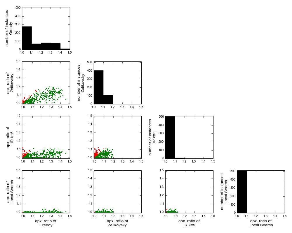
Figure 1 shows comparison of approximation ratios of four main algorithms: greedy 2-approximation, Zelikovsky algorithm, Local Search and IR for . We define approximation ratio as cost of algorithm solution divided by best known cost from SteinLib. The figure shows only those cases for which all algorithms were able to find solutions within the time limit, so there are points. There are four histograms and we can easily see that for test cases from SteinLib Local Search achieves the best results, being slightly better than Iterative Rounding.
Every point on each of scatter plots represents one test case with its approximation ratios on and axis. We can see that there are cases for which Iterative Rounding performs better than Local Search.
Table 2 shows average approximation ratios and running times in seconds for each difficulty class, as defined in SteinLib [17].
| Class | Greedy | Zelikovsky | IR | IR | Local Search | ||||
|---|---|---|---|---|---|---|---|---|---|
| optimized | |||||||||
| ratio | time | ratio | time | ratio | time | ratio | time | ratio | |
| ?? | 1.139 | 0.001 | 1.028 | 0.000 | 1.000 | 29.250 | 1.000 | 3.080 | 1.000 |
| ?m | 1.338 | 0.161 | 1.133 | 5.815 | 1.040 | 105.350 | 1.040 | 11.395 | 1.002 |
| ?s | 1.035 | 0.002 | 1.016 | 0.103 | 1.030 | 90.537 | 1.030 | 29.706 | 1.001 |
| Lm | 1.317 | 0.034 | 1.105 | 0.400 | 1.048 | 7.320 | 1.048 | 1.170 | 1.000 |
| Ls | 1.036 | 0.001 | 1.008 | 0.002 | 1.014 | 138.262 | 1.011 | 70.991 | 1.000 |
| NP? | 1.175 | 0.001 | 1.056 | 0.025 | 1.017 | 64.228 | 1.017 | 36.947 | 1.000 |
| NPm | 1.294 | 0.007 | 1.089 | 0.212 | 1.047 | 61.596 | 1.047 | 26.438 | 1.003 |
| NPs | 1.267 | 0.001 | 1.097 | 0.008 | 1.036 | 80.695 | 1.038 | 49.201 | 1.001 |
| Ph | 1.200 | 0.043 | 1.067 | 5.090 | 1.000 | 25.530 | 1.000 | 16.390 | 1.000 |
| Pm | 1.266 | 0.054 | 1.100 | 1.563 | 1.033 | 75.500 | 1.033 | 8.038 | 1.005 |
| Ps | 1.188 | 0.002 | 1.071 | 0.030 | 1.029 | 46.461 | 1.028 | 18.692 | 1.002 |
| Average | 1.152 | 0.005 | 1.057 | 0.161 | 1.030 | 67.677 | 1.029 | 26.490 | 1.001 |
7.2 Approximation Ratio of Iterative Rounding Depending on
Figure 2 shows approximation ratios of IR depending on the value of . On average, with increasing approximation ratio gets closer to . There are some cases, where for bigger IR gives worse results (we need to remember, however, that the IR is a randomized approximation algorithm). Table 3 shows average approximation ratios and average running times of Iterative Rounding for different values of and different SteinLib dificulty classes.

| Class | IR | IR | IR | IR | ||||
|---|---|---|---|---|---|---|---|---|
| ratio | time | ratio | time | ratio | time | ratio | time | |
| ?? | 1.361 | 0.020 | 1.000 | 0.090 | 1.028 | 2.290 | 1.000 | 3.080 |
| ?m | 1.338 | 6.945 | 1.132 | 7.100 | 1.084 | 8.805 | 1.040 | 11.395 |
| ?s | 1.126 | 7.537 | 1.044 | 10.317 | 1.033 | 28.813 | 1.030 | 75.684 |
| Lm | 1.317 | 0.440 | 1.108 | 0.460 | 1.055 | 0.920 | 1.048 | 1.170 |
| Ls | 1.083 | 0.333 | 1.024 | 0.667 | 1.011 | 10.161 | 1.008 | 57.596 |
| NP? | 1.371 | 1.125 | 1.045 | 16.150 | 1.029 | 26.250 | 1.017 | 36.947 |
| NPh | 1.321 | 0.240 | 1.134 | 0.570 | 1.095 | 5.800 | 1.098 | 38.010 |
| NPm | 1.353 | 0.243 | 1.095 | 0.515 | 1.061 | 3.909 | 1.051 | 31.811 |
| NPs | 1.282 | 0.085 | 1.103 | 0.318 | 1.053 | 4.280 | 1.040 | 50.315 |
| Ph | 1.213 | 9.810 | 1.060 | 8.770 | 1.060 | 40.855 | 1.020 | 122.940 |
| Pm | 1.311 | 1.968 | 1.123 | 1.954 | 1.068 | 8.530 | 1.040 | 25.519 |
| Ps | 1.233 | 0.356 | 1.068 | 0.464 | 1.046 | 6.172 | 1.027 | 34.033 |
| Average | 1.202 | 2.211 | 1.063 | 3.111 | 1.041 | 12.307 | 1.028 | 47.527 |
7.3 Results
Comparing the 3 approximation algorithms implemented as a part of this work we see that for big enough parameters (), the results returned by the IR algorithm are better then those returned by both the greedy and Zelikovsky algorithms.
On the other hand, the running times of the IR algorithm are much higher then for the other two algorithms. Also, while both the greedy and Zelikovsky algorithms were able to solve over 90% of SteinLib instances within our 10 minute time limit, the IR for solved only 60% of the instances, and that number decreases for bigger values of .
The MS Local Search heuristics from [22] gives, on average, lower costs then all of the algorithms with theoretical guarantees we have implemented. It was also able to solve all SteinLib instances in under 3 minutes. Note, however, that the paper [22] gives 12 different versions of the local search and only the best one of them visibly outperforms our IR algorithm. The other ones give worse or comparable results.
Additionally, we have compared our IR results with few other papers. Our algorithm for gives better results then the Tabu Search from [2], whereas it improves slightly over the results from [8] only on incidence class of SteinLib instances.
To summarize, the Iterative Rounding 1.39-approximation algorithm, which was the main interest of this paper, does seem to give approximation results that compare decently with other approaches. It is only outperformed by the best of Local Search implementations. However, despite good theoretical approximation ratio and decent experimental quality of solutions, it’s running time is visibly higher then the one of the state-of-the-art heuristics like Local Search algorithms. Nevertheless, the most important goal of this study, i.e., to demonstrate that high-level approximation algorithm concepts can be implemented efficiently was accomplished successfully. Having implementations of these concepts available it is easier to continue the work on hybrid solutions that would combine the best aspects of different approaches and could potentially lead to better results.
8 Acknowledgements
We would like to thank Jarek Byrka for helpful comments on our optimization of components generation.
References
- [1] M. Andrejczuk. Implementation of the dreyfus-wagner algorithm for the steiner tree problem, August 2014. http://paal.mimuw.edu.pl/dreyfus__wagner_8hpp_source.html.
- [2] Marcelo P Bastos and Celso C Ribeiro. Reactive tabu search with path-relinking for the steiner problem in graphs. In Essays and surveys in metaheuristics, pages 39–58. Springer, 2002.
- [3] Attila Bernáth, Krzysztof Ciebiera, Piotr Godlewski, and Piotr Sankowski. Implementation of the iterative relaxation algorithm for the minimum bounded-degree spanning tree problem. In Experimental Algorithms - 13th International Symposium, SEA 2014, Copenhagen, Denmark, June 29 - July 1, 2014. Proceedings, pages 74–86, 2014.
- [4] Jarosław Byrka, Fabrizio Grandoni, Thomas Rothvoss, and Laura Sanità. Steiner tree approximation via iterative randomized rounding. J. ACM, 60(1):6:1–6:33, February 2013.
- [5] Miroslav Chlebik and Janka Chlebikova. The steiner tree problem on graphs: Inapproximability results. Theoretical Computer Science, 406(3):207 – 214, 2008. Algorithmic Aspects of Global Computing.
- [6] Krzystof Ciebiera, Piotr Sankowski, and Piotr Wygocki. C++11 generic local search framework case study. unpublished.
- [7] M Poggi de Aragao, Celso C Ribeiro, Eduardo Uchoa, and Renato F Werneck. Hybrid local search for the steiner problem in graphs. In Extended abstracts of the 4th metaheuristics international conference, pages 429–433, 2001.
- [8] Marcus Poggi de Aragão and Renato F Werneck. On the implementation of mst-based heuristics for the steiner problem in graphs. In Algorithm Engineering and Experiments, pages 1–15. Springer, 2002.
- [9] Karel Driesen and Urs Hölzle. The direct cost of virtual function calls in c++. SIGPLAN Not., 31(10):306–323, October 1996.
- [10] Ding-Zhu Du, JM Smith, and J Hyam Rubinstein. Advances in Steiner trees, volume 6. Springer, 2000.
- [11] Cees Duin and Stefan Vo. Efficient path and vertex exchange in steiner tree algorithms. Networks, 29(2):89–105, 1997.
- [12] EN Gilbert and HO Pollak. Steiner minimal trees. SIAM Journal on Applied Mathematics, 16(1):1–29, 1968.
- [13] GLPK (GNU Linear Programming Kit). https://www.gnu.org/software/glpk/.
- [14] Michel X. Goemans, Neil Olver, Thomas Rothvoß, and Rico Zenklusen. Matroids and integrality gaps for hypergraphic steiner tree relaxations. In Proceedings of the Forty-fourth Annual ACM Symposium on Theory of Computing, STOC ’12, pages 1161–1176. ACM, 2012.
- [15] M. Grötschel, L. Lovász, and A. Schrijver. The ellipsoid method and its consequences in combinatorial optimization. Combinatorica, 1(2):169–197, 1981.
- [16] Kamal Jain. A factor 2 approximation algorithm for the generalized steiner network problem. Combinatorica, 21(1):39–60, 2001.
- [17] T. Koch, A. Martin, and S. Voß. SteinLib: An updated library on steiner tree problems in graphs. Technical Report ZIB-Report 00-37, Konrad-Zuse-Zentrum für Informationstechnik Berlin, Takustr. 7, Berlin, 2000.
- [18] Lap Chi Lau, Ramamoorthi Ravi, and Mohit Singh. Iterative methods in combinatorial optimization. Cambridge University Press, 2011.
- [19] Kurt Mehlhorn. A faster approximation algorithm for the steiner problem in graphs. Information Processing Letters, 27(3):125 – 128, 1988.
- [20] P. Smulewicz P. Wygocki. Implementation of the greedy 2-approximation for the steiner tree problem, August 2014. http://paal.mimuw.edu.pl/steiner__tree__greedy_8hpp_source.html.
- [21] Jeremy G Siek, Lie-Quan Lee, and Andrew Lumsdaine. Boost Graph Library: User Guide and Reference Manual, The. Pearson Education, 2001.
- [22] Eduardo Uchoa and Renato F. Werneck. Fast local search for the steiner problem in graphs. J. Exp. Algorithmics, 17:2.2:2.1–2.2:2.22, May 2012.
- [23] Vijay V. Vazirani. Approximation Algorithms. Springer-Verlag New York, Inc., New York, NY, USA, 2001.
- [24] MGA Verhoeven, MEM Severens, and EHL Aarts. Local search for steiner trees in graphs. Modern Heuristics Search Methods, pages 117–129, 1996.
- [25] P. Wygocki. Implementation of the 11/6 approximation for the steiner tree problem, August 2014. http://paal.mimuw.edu.pl/zelikovsky__11__per__6_8hpp_source.html.
- [26] Alexander Z Zelikovsky. An 11/6-approximation algorithm for the network steiner problem. Algorithmica, 9(5):463–470, 1993.