Measurement of the Shape Factor for the Beta Decay of 14O
Abstract
We report results from an experiment designed to test the conserved vector current (CVC) hypothesis by measuring the shape of the -decay spectrum for the allowed ground state decay of 14O. Measurements of the spectrum intensity were obtained with a superconducting beta spectrometer and will be reported for positron kinetic energies ranging from 1.9 to 4.0 MeV. After dividing out phase space, Coulomb, and other correction factors, the resulting shape function has a negative slope of several per cent per MeV. We define a parameter , which is essentially a measure of the average slope of the shape function over the energy range of the measurements, and determine its value to be (stat.) (syst.). The measured slope parameter is in good agreement with predictions from shell model calculations that respect CVC.
pacs
23.40.Bw, 23.40.-s, 24.80.+yI Introduction
The nucleus 14O has a half-life of 70.62 s [1] and decays by positron emission. More than 99% of the decays proceed by a Fermi transition from the 14O ground state to the isobaric analog 2.313 MeV first excited state of 14N. The ground state branch, which is the subject of the present work, is an allowed Gamow-Teller (GT) transition with an endpoint energy of 4.12 MeV, and a log value of roughly 7.3. The unusually large is thought to be the result of an accidental cancellation between various nuclear wave function components that contribute to the axial vector matrix element [2, 3].
Because the allowed GT matrix element, , is suppressed, contributions from ordinarily small forbidden matrix elements may well be appreciable, and could lead to deviations of the beta spectrum from the purely statistical shape.
Of particular interest is the contribution from the (vector) weak magnetism (WM) term. The WM matrix element affects the spectrum shape through interference with the dominant GT matrix element (see for example Ref. [4]) giving rise to an extra energy dependent shape factor,
| (1) |
where () is the nucleon (electron) rest energy, is the total electron energy, and is the corresponding endpoint energy. The quantity is the WM matrix element, where is defined in Ref. [4] and .
In 1958, Gell-Mann [5] proposed that measurements of in systems like the present one can, in principle, allow a test of the conserved vector current (CVC) hypothesis [6]. CVC implies that the WM operator is identical to the electromagnetic M1 operator that determines the lifetime of the 2.313 MeV state in 14N. Assuming CVC and charge symmetry, one would have , with known from the measured -decay width.
Following Gell-Mann’s suggestion, a number of experimental groups [7, 8, 9, 10] undertook experiments to measure -decay shape factors in the system. Unfortunately, results from the different groups show discrepancies well beyond the quoted uncertainties, demonstrating the extreme difficulty of experiments of this kind.
Calaprice and Holstein [4] have calculated for a series of nuclei and found that the ratio should be an order of magnitude larger for 14O than for the nuclei. From the experimental point of view, this makes the 14O experiment attractive. On the other hand, given that is so small, one needs to be concerned about possible energy dependences that can arise from the various higher order matrix elements (for example, second forbidden terms) or from other normally negligible effects such as charge symmetry violation.
Tests of CVC are of central importance and this provides the fundamental motivation for the present experiment. According to CVC, the weak charge-changing vector currents together with the electromagnetic current make up a 3 component isospin multiplet. This symmetry leads to the result. CVC has other consequences as well, such as the non-renormalization of the weak vector current, but experiments are considered strong tests of CVC [11]. Previous 14O measurements (from the mid 1960’s) have been reported [12], but in view of the importance of the subject we believe that a second measurement of the spectrum shape would be valuable, particularly since recent analyses have suggested that there may be systematic problems with these measurements.
Measurements of the -spectrum of 14O are important for a second reason. The excited state decay is one of the superallowed Fermi transitions used to determine the element of the CKM matrix, and the analysis requires knowledge of the 14O branching ratio. We will report new results for that quantity in a subsequent publication.
II Summary of Previous Work
Measurements of the shape of the spectrum of 14O were reported in 1966 by Sidhu and Gerhart [12] (SG). These authors used an iron-free, uniform-field, solenoidal spectrometer to focus positrons emitted from a source that was produced by freezing 14O water onto a liquid-nitrogen-cooled beryllium disc. Positrons passing through the spectrometer were detected with a plastic scintillator approximately 1 cm thick. Corrections for backscattering from the source backing, for -ray backgrounds, and for sub-threshold positron events were included in the data analysis.
The experimental results summarized in Figure 6 of Ref. [12] show significant deviations from the purely allowed (statistical) shape. The authors plot the quantity
| (2) |
where is the number of detected positron events (normalized for variations in source activity and counting time), and where is the Fermi function. The “extra” factor of in the denominator is included to account for the fact that the momentum acceptance width of the spectrometer scales with .
The experiment shows to be a monotonically decreasing quantity with a relative slope of typically 9% per MeV; more specifically, if we compare the reported measurements with a function of the form given in Eq. (1),
| (3) |
the results indicate a slope parameter of about 0.09/MeV. This is roughly a factor of 2 larger than the naive CVC prediction from Ref. [4]. However, it should be noted that this comparison does not take into account various modern corrections to the beta spectrum shape. In particular, as we shall discuss later, corrections for radiative processes are not negligible.
On the theoretical side, García and Brown [13] (GB) have carried out a detailed study of the -spectrum shapes and values. One of the long-standing issues in mass 14 is the large asymmetry in the values for the 14C and 14O decays. It is thought that the cancellations in the dominant GT matrix element may be very sensitive to small wave function differences that can arise from charge symmetry violations and/or Coulomb effects. GB investigate whether these same effects may also be responsible for the unexpectedly large 14O -decay slope parameter. They conclude that these effects can be no more than a few per cent for and . The slopes they find in calculations that respect charge symmetry and CVC are at least a factor of 1.7 smaller than the measured slope.
Towner and Hardy [14] (TH) have reported a new analysis of the 14O -decay data. They, for the first time, apply corrections for radiative processes as well as several other small effects. Nevertheless, they still agree with the general conclusions of GB when free-nucleon operators are used in their calculations. Attempts to reproduce the SG data seem to require violation of CVC.
On the other hand, when renormalized operators are used for the GT and WM matrix elements, the results improve significantly. It is known [15] that, in finite nuclei, the effective axial vector coupling constant is depressed (compared to the free nucleon value) by core polarization and meson exchange currents, and it is expected that the M1 and WM operators also need to be renormalized. TH use the known GT renormalization factor along with M1 renormalization parameters from Ref. [16], and fit the decay data of Ref. [12] with only a single adjustable wave function parameter. In doing so, they are able to reproduce the overall transition rate and obtain a value consistent with CVC, while underpredicting the measured slope by only around 20% instead of by almost a factor of two.
As we suggested earlier, contributions from higher order matrix elements may be of importance in 14O decay. GB include two higher order terms in in their analysis, and it appears to us (from calculations based on formulas presented by GB) that these terms have a significant effect on the slope parameter. TH do not explicitly separate out the higher order pieces, but their results also suggest that these terms are important. In particular, their calculations predict the presence of an term in the shape-correction function which is an order of magnitude larger than one would obtain if only the GT and WM terms are present.

III Experimental Details
The new measurements were carried out at the University of Wisconsin Nuclear Physics Laboratory. Radioactive 14O was produced by bombarding a 14N gas target with a proton beam of typically 8 MeV obtained from the Wisconsin tandem electrostatic accelerator. A significant fraction of the 14O atoms were incorporated into water molecules in the production cell. Gas from the production cell was then periodically transported through a capillary tube to a separation trap, and the H2O molecules were subsequently transported to a beta spectrometer where the measurements were carried out. The details will be given below.
III.1 Superconducting Beta Spectrometer
The spectrometer used in the present experiment has been described in detail elsewhere [17]. A schematic diagram that illustrates some of the relevant details is shown in Fig. 1. The spectrometer design follows the basic principles of the “Wu Spectrometer” described in a 1956 paper by Alburger [18], with fields provided by a set of superconducting magnet coils.
The magnetic fields in the spectrometer are shaped to provide angle focusing and momentum dispersion of positrons or electrons at the midplane. Curves shown in Fig. 1 depict the trajectories of positrons emitted from the source position at angles in the neighborhood of . These curves display the and coordinates of the trajectories, while in reality the particles also spiral around the magnetic field lines. Positrons of the appropriate momentum are focused at the midplane slits, and after passing through the aperture are re-focused onto a detector.
The acceptance of the spectrometer is defined by a pair of “entrance slits” that limit the angular acceptance, and a second pair of slits at the midplane that do the momentum selection. The slits are made of 3.2 mm thick copper and are machined at angles so that passing positrons do not strike the slit edge. Since the spectrometer is iron-free, the centroid of the momentum acceptance function scales accurately with current. For a current of 10 A, the acceptance function peaks at approximately 2.48 MeV/c. Under the conditions of the present experiment the acceptance function has a FWHM of about 2%, and a peak solid angle of roughly 0.5 sr. The calibration of the spectrometer (momentum vs. current) has been determined to better than 1 part in . The calibration procedure and many additional details concerning properties and operation of the spectrometer are described in Ref. [17].
Detection of positrons that pass through the spectrometer slits is accomplished with a nominally 1 cm diameter, 5 mm thick lithium-drifted silicon [Si(Li)] detector. Signals from the detector are processed with a preamplifier followed by a linear amplifier and some gating electronics. The signals are then analyzed with a peak-sensing analog-to-digital converter (ADC) which is read out by a computer.
The activity in the spectrometer is monitored with a 7.5 cm diameter, 5 cm thick BGO scintillator that is used to detect 2.3 MeV -rays emitted following 14O decay to the 14N first excited state. This detector is heavily shielded against backgrounds, and is located at a point where it detects -rays that originate near the source position. The signals from this detector are also processed through an ADC which is read out into the computer.
III.2 Source Preparation
To obtain measurements of the beta spectrum we need to prepare 14O sources and insert them into the counting position as shown in Fig. 1. Accurate positioning of the source is critical. For example, a vertical offset of 0.1 mm would lead to an unacceptable momentum shift of 5 parts in . Furthermore, in view of the short half-life, the preparation and insertion of new sources obviously needs to be repeated many times.
In the present experiment, the source consists of 14O water deposited and frozen onto a 3 mm diameter spot at the center of a 13 thick aluminum foil. The foil is suspended across a 15 mm diameter hole in a copper source holder, and attached to the source holder with epoxy. To prevent sublimation of the water, the source holder is cooled to typically 140 K by thermal contact with “catchers” at liquid nitrogen temperature. We use aluminum because it has a greater coefficient of thermal expansion than copper. The consequence is that when the source mechanism is cooled, the foil stretches tightly across the opening in the holder, minimizing possible longitudinal position errors.
The source holder can be moved between two positions. In the lower position, 14O water is loaded onto the foil, while the upper location is the counting position. In both locations the source holder is positioned by direct mechanical contact with a catcher which centers the foil horizontally and fixes the vertical position.
Since 14O has a short lifetime, the source holder is cycled between the loading and counting positions at frequent intervals. For most of the measurements presented in this paper the cycle time was 140 s. During a given cycle the source was in the upper and lower positions for about 105 s and 25 s, respectively, with about 5 s for each transition.
To make a transition, the source holder is first retracted, the entire mechanism is then rotated through , and finally the source is extended, making contact with a catcher. A simple pneumatic gas piston is used to retract and extend the source, while the rotation is accomplished with a vacuum feedthrough coupled to a stepping motor. In the counting position the source spot is on the upper surface of the aluminum foil, so that positrons do not pass through the foil.
While the foil position is supposedly fixed by contact with the catcher, complete insertion of the source holder sometimes takes place slowly and can, at times, fail entirely. To eliminate the resulting bad sections of data, the extension of the source holder is measured and recorded every 0.1 s. This is accomplished with a pair of small, concentric mutual induction coils, one attached to the source holder and the other to the source motion mechanism. A sinusoidal voltage is applied to the primary coil and the induced signal in the secondary is rectified, integrated and amplified, and the resulting DC signal is processed through an ADC.
The source motion mechanism is designed to minimize positron backscattering by keeping the amount of material behind the source in the acceptance cone of the spectrometer to a minimum. In particular, the source holder is supported by two thin brass rods which couple the source to the mechanism.
Within each cycle, various operations take place at not only the spectrometer but also at the production cell and water separation trap. All of the activities are automated, taking place under control of a computer.
Figure 2 shows some of the gas handling details. For most of each cycle, the production cell is filled at a pressure of about 220 kPa with nitrogen gas which has been admixed with about 0.2% hydrogen. The cell volume is with a pathlength for beam protons of about 10 cm. Within the cell much of the gas is ionized by the beam (usually 1.0 or 1.5 ), and one finds that a significant fraction of the 14O produced gets incorporated into water, provided that the levels of CO2 and O2 (which efficiently scavenge 14O) are sufficiently low.
As 14O is being produced, gas is slowly drawn out of the cell through a 7 m long teflon capillary tube with an inside diameter of 0.8 mm. Water in the gas mixture is trapped at a point where a single loop of the teflon tube, 2 or 3 cm in length, dips into an alcohol bath at a controlled temperature of -70 C. Nitrogen and other gasses that are not trapped pass through a switching valve and a needle valve to a pump.

At some point in the cycle we wish to empty the cell and send the accumulated 14O water to the spectrometer. The sequence is to close the nitrogen inlet valve at the production cell and simultaneously open a bypass valve to increase the gas flow through the teflon tube. After 3 seconds the cell pressure is partially reduced and the cell is purged with a puff of helium gas followed 3 seconds later by a second puff. After another few seconds the condensed water is liberated by moving the teflon loop from the cold bath to a hot water bath at +80 C. Then, at the appropriate moment the switching valve is activated, routing the output gas to a second 0.8 mm diameter teflon tube that leads to the spectrometer. The timing parameters are all carefully adjusted so that there is still an adequate flow of helium from the production cell to sweep the water molecules along to the spectrometer.
The capillary tube leading to the spectrometer was 8 m long for our initial data acquisition runs and 5 m long in later runs. The tube terminates about 2 mm below the lower source position so that the jet of helium and water is sprayed directly onto the source foil. Here, a 3 mm diameter aperture directly in front of the foil limits the size of the active spot to that diameter. Measurements indicate that typically to of the 14O activity ends up on the source foil. Most of the remaining activity probably remains frozen on the collimator, which is outside the field of view of the spectrometer. The source foil activity was typically a few times Bq at the start of a counting interval.
After the 14O has been loaded onto the foil and most of the residual gas pumped away, the source is moved to the upper position. Over time, an easily visible 3 mm diameter ice spot appears on the aluminum foil. Of course, besides the 14O water our system also traps water that forms from oxygen that outgasses from the walls of the production cell. In order to reduce backscattering of positrons from this ice, the foil is warmed to near room temperature every few hours. To get some idea of how much material had collected on the foil we combine measurements of the pressure rise as a function of time during the warming period with an estimate of the pumping speed. The conclusion is that the thickness of ice was generally less than 2 mg/cm2.
III.3 Computer System
A dedicated computer equipped with analog and digital I/O boards is used to control the experiment and collect data. The computer performs many jobs. It controls the valves in the gas handling system and the motion of the water separation trap. It initiates retraction, rotation and extension of the source motion mechanism and monitors the resulting foil position. It measures the current in the superconducting magnet and sends feedback signals to the magnet power supply to regulate the current at the desired value. It reads digital information from the Si(Li) and BGO ADCs and issues the appropriate reset signals. Finally it provides run start and stop signals to external electronics, and shuts down the superconducting magnet if temperatures drift too high.
A second dedicated computer is used to view the incoming data in real time. We do this to avoid the use of graphics displays on the control computer, which create excessive dead time. The two computers communicate through an internet link.
The control computer also carries out the task of saving incoming data into an event stream. The event stream consists of a series of records corresponding to events of various kinds. Recorded events include ADC outputs, measurements of the magnet current and the foil position, plus run start and stop commands. Each record includes an event-type identifier and a timestamp.
III.4 Measurement Procedure
Measurements will be reported for currents ranging from 9.5 to 18.0 A, corresponding to positron momenta of 2.36-4.46 MeV/c. At lower currents one begins to encounter positrons from decay to the 14N first excited state. Some data were also taken at 18.5 and 19.0 A, currents which are near or above the endpoint of the ground state transition.
Data acquisition was divided into a series of runs with lengths anywhere from 20 to 45 minutes, allowing for a number of 140 s cycles. Recall that our goal is to determine the shape of the ground state beta decay spectrum, and for that purpose we want to measure ratios of counting rates at different spectrometer settings. Thus within any given run we take measurements at anywhere from 2 to 6 different magnet currents.
Once a newly prepared source has been inserted into the counting position we have roughly 105 s to observe decay positrons. During each 105 s counting period we cover all currents of interest for that particular run, first counting, then ramping to the next current, counting, ramping, and so on. All of this is timed to complete the last current just before the counting period ends and the source is retracted for re-loading.
The spectrometer magnets have an inductance of 12 H, and consequently the ramping times are not small. Therefore we alternate between “up ramps”, from low to high currents, for one cycle, and “down ramps”, from high to low, for the next.
Many different current combinations (or ramping modes) were employed in our data productions runs. For example, Mode 1 covers currents of 11.0, 11.5 and 12.0 A, while modes 2, 3 and 4 use 6 currents separated by 1.5 A starting at 9.5, 10.0, or 10.5 A. Runs of this kind allow us to cover the region of interest with the spectrum shape fixed either by directly measured ratios, or by ratios of ratios. In all, around 20 different ramp modes were used at one time or another.
The data to be presented here were obtained in a series of 4 running periods, two in July of 2012, and two more in February and March of 2014. New features added for the 2014 runs include: 1) run-by-run monitoring of the “sticking fraction”, the fraction of the 14O activity deposited onto the source foil; 2) a more careful measurement of beam-associated background in the Si(Li) detector; and 3) the use of a shorter delivery tube to the spectrometer.
III.5 Sample Spectra

As noted above, a BGO detector located outside the spectrometer is used to monitor the source activity. A typical energy spectrum obtained with this detector (Run 6454) is shown in Fig. 3. Here we see a single strong peak, just above channel 100, corresponding to 2.3 MeV -rays emitted following beta decay to the first excited state of 14N. Above the peak there are counts which arise primarily from beam associated background. Although the BGO detector is separated from the production cell by a thick shielding wall, some neutrons produced by the beam thermalize, diffuse into the spectrometer hall, and capture in various objects. The capture -rays produce background in the BGO and, to some extent, in the Si(Li) detector as well. In our analysis of the data (see Sect. V below) we use the counting rate in this upper region of the BGO spectrum as an aid to help us eliminate the corresponding Si(Li) detector background.
If we set a window around the 2.3 MeV peak, we can monitor the source activity. In Fig. 4 we show the counting rate inside this window as a function of time for a portion of Run 6454. We see initial counting rates between 150 and 200 Hz, with the activity decaying as expected. The lower source position is outside the field of view of the detector, so the rate drops to near zero when the source is removed for re-loading.

In Fig. 5 we show some of the Si(Li) spectra obtained during Run 6454. These spectra have an energy gain of approximately 10 keV per channel. In this particular run, data were taken at 6 currents separated by 1.5 A and starting at 9.5 A. The plot shows the accumulated spectra for 3 of the 6 current settings, and the main feature of interest is a peak corresponding to the full kinetic energy of the positrons. The run shown comprised 12 cycles and the accumulated counting time at each current was about 150 s. Since we alternate upward and downward ramps, the net number of 14O decays at the various currents are the same to within about 10%.

The counts in Fig. 5 below channel number 100 are almost entirely background, the main sources of which are 511 keV gamma rays and positrons from decay of 11C. The presence of counts from 11C, which has an endpoint energy of 960 keV, requires some explanation. Under the conditions of our experiment we produce large amounts of 11C via the reaction. Most of the 11C is probably incorporated into molecules such as HCN, CO, CO2 or CH4 which would not freeze out in our water separation trap, and should therefore be pumped away.
Now, before sending gas to the spectrometer we attempt to pump the cell and purge it with helium, but some 11C certainly remains and can be carried to the spectrometer along with the desired remnant helium gas. Any 11C deposited on the source foil is of little consequence, since the positron momentum is far too low for the spectrometer settings represented in Fig. 5. However, some 11C must enter the spectrometer itself. The teflon tube that delivers the 14O is very long and thin, and consequently some of the 11C/helium mix continues to flow from the tube as the source holder begins moving to the counting position. Any gas that emerges during the 5 s transition time is likely to enter the spectrometer. From there the 11C molecules diffuse around and are either pumped away or adsorbed onto some surface. Based on detailed Monte-Carlo simulations, we conclude that the counts we observe come from 11C deposited very close to the detector, possibly even on its front surface. That hypothesis explains the shape of the observed low-energy Si(Li) spectrum and the fact that the rate is very nearly independent of the spectrometer current.
The spectra shown in Fig. 5 were obtained during one of the 2012 running periods. For the 2014 running periods, the delivery tube to the spectrometer was shorter and the 11C background was reduced by typically a factor of two or more.

Sample Si(Li) spectra with improved statistics are shown in Fig. 6. This figure shows the combined spectra for all data taken at currents of 10 and 16 A. In each case there is a prominent peak corresponding to events in which the positron deposits its full kinetic energy in the detector. The wider peak at 16 A reflects the increasing momentum acceptance of the spectrometer with current.
The counts above the main peak arise from processes in which the positron energy pulse is supplemented with energy deposited in the detector by one or both annihilation -rays. Below channel 130 we see counts from 11C decay. The broad structure between channels 140 and 320 seen at 16 A is the “” bump, arising from positrons that pass through the active silicon without depositing full kinetic energy. Finally the counts below the 10 A peak between channels 130 and 190 are primarily from positrons that backscatter out of the detector.
IV Background Processes
Briefly stated, the goal of our data analysis is to determine the shape of the 14O ground-state beta decay spectrum from measurements of the kind shown in Fig. 5. To accomplish this we first need to eliminate background counts. In addition, there are various corrections that need to be applied. For example, there are processes that allow positrons emitted outside the normal spectrometer acceptance to reach the detector and contribute to the counting rate. We begin with a discussion of the backgrounds.
Background counts can arise from a number of sources. We have already seen the effects of positrons from 11C and of 511 keV -rays. The counting rates from these processes are high, but fortunately the counts are confined to the low-energy parts of the Si(Li) spectra. At higher energies, we need to account for room background from cosmic rays and radioisotopes such as 40K, backgrounds associated with the beam, and counts from 2.3 MeV -rays emitted following excited state decay of 14O.
IV.1 2.3 MeV Gamma-Rays
The great majority of all 14O beta decays branch to the first excited state of 14N, and are then followed by emission of a 2.3 MeV -ray. The ground state branching ratio is only about 0.5% and therefore we have approximately 200 -rays for each positron of interest. The flux is greatly attenuated by the lead shadow bar located between the source and Si(Li) detector, and the rate is further reduced by the small size and low of the detector. Nevertheless, 2.3 MeV -rays are a significant source of background.
We have no way to measure this background directly, and so we are forced to rely on Monte-Carlo simulations. The present simulations, as well as others described later in this paper, were carried out with one of two separate codes developed at Wittenberg and Wisconsin, both based on EGSnrc [19].
The main process by which the 2.3 MeV -rays produce detector counts in the energy range of interest is by Compton scattering from material near the spectrometer midplane slits (see Fig. 1). When the scattering occurs near the upper surface of a slit or the support structure, ejected electrons can follow field lines to the detector.
Results from the Monte-Carlo simulation of the 2.3 MeV -ray events are shown in Fig. 7 along with some of the other important background corrections. The results presented are for a spectrometer current of 10 A, and the number of decays, , has been chosen to match the 10 A spectrum of Fig. 6.

In our -ray simulations we see no counts above the 2.3 MeV Compton edge, corresponding to channel 208 in our spectra. As we increase the spectrometer current, the 14O positron peak moves up in energy, whereas the counts are still confined to the region below the Compton edge. We also find that the number of events decreases with increasing current.
Besides the 14O on the source foil, many 14O atoms freeze out in the general area of the source loading position, and of course, the -rays emitted from that location can also produce background counts in the Si(Li) detector. Our simulations of this process give spectra similar to those for -rays from the source position, except that the counting rate is reduced by roughly an order of magnitude.
Fortunately we have the possibility of doing a check on the reliability of the -ray simulations. During data acquisition time, we took a number of runs in which the source foil was not moved away from the source loading position. In this case, 14O accumulates on the foil and the surrounding area. From that position no positrons can reach the Si(Li) detector, so the spectrum should be purely background. During these “foil-down runs” we normally recorded the spectrum from a second BGO detector positioned to observe 2.3 MeV -rays that originate from near the loading position. When coupled with Monte-Carlo calculations of the efficiency of the detector in this geometry, we get a measure of the total 14O activity.

In Fig. 8 we show the combined Si(Li) spectrum from two such runs with the spectrometer current set at 10 A. From the corresponding BGO spectra we conclude that these runs comprised a total of about decays. Along with the experimental data we show the result from a Monte-Carlo simulation of the process. The simulation spectrum shown includes counts from the 2.3 MeV -rays plus measured room and beam backgrounds (see Sect. IV.2 below). Given that the foil motion mechanism is quite complex and not accurately modeled in our simulation codes, and that the spatial distribution of the decaying atoms is not well known, we consider the agreement between the measurements and simulation to be surprisingly good.
IV.2 Other Backgrounds
The spectrum in panel (b) of Fig. 7 shows the combined room and beam-associated backgrounds. The beam-off room backgrounds were measured directly in a series of long runs that were interspersed between the data acquisition runs. The resulting Si(Li) rates, integrated between channels 130 and 450, are on the order of 0.015/s. These background spectra appear to be independent of the spectrometer current, but the overall rates rise very slowly during any given data acquisition period, presumably from activation of the surrounding materials by neutron capture.
The beam-associated background is of about this same order of magnitude. For the 2012 data, this spectrum was measured during a separate running period a few months after the data acquisition periods. During this run we accumulated Si(Li) spectra for many hours at different spectrometer currents with beam on and beam off. As in the case of the room background, it appears that the beam-associated background is independent of the spectrometer current. In 2014, the beam-on backgrounds were measured from time to time during the data acquisition period.
It is expected that the beam background can vary from run to run, as the beam energy, current and focusing change. However, we believe that the Si(Li) beam background and the counts in the upper portions of the BGO spectrum (above channel 200 in Fig. 3) both arise from -rays from thermal neutron capture. Therefore, the procedure we use is to compute, for each run, the BGO rate summed typically between channels 225 and 450. We then scale the beam background spectrum by the ratio of that rate to the corresponding BGO rate observed during the measurement of the beam-on background. The scale factors were typically 1 to within 10%.
IV.3 Corrections for Bad Events
We now come to the subject of backgrounds that arise from positrons. In the simplest picture, Si(Li) counts occur when positrons emitted from the source pass between the spectrometer slits and reach the detector without striking any other object. We call these “good events”. There are other ways in which positrons can produce Si(Li) counts. Several of the mechanisms are described in detail in Ref. [17]. The possibilities include scattering from slit edges, backscattering from the source foil, and the detection of -rays from annihilation of positrons that do not reach the detector. These and other processes give rise to the “bad events”.
The good events arise from positrons emitted into a well-defined momentum and angle window, with a momentum acceptance that scales directly with the spectrometer current. The spectrometer acceptance for good events is called the “geometrical acceptance.” In contrast, the bad events have no simple dependence on current. Consequently, before making a direct comparison between counting rates at different currents we need to remove or correct for the bad events. As we did for the 2.3 MeV -rays, we determine these corrections from Monte-Carlo simulations.
The simulated bad-event spectrum at 10 A is shown in panel (c) of Fig. 7. Once again, the number of events has been chosen to match the 10 A spectrum of Fig. 6. The bad-event spectrum has a number of interesting features. In particular there is a clear peak just below channel 160. These events arise from a process described previously in Ref. [17]. Positrons emitted close to and with about 83% of the nominal acceptance momentum make extra loops in the magnetic field and can pass through all of the spectrometer slits. These positrons eventually hit the lead shadow bar (see Fig. 1) and some fraction “bounce” off and reach the detector.
Ordinarily, the Si(Li) spectrum has very few of these “loopy” events. However at currents below 11 A, the acceptance for the loopy events is below the endpoint for excited state positron decays, leading to a greatly increased event rate. For example, at 10 A, the enhancement factor is 50, and one can see an indication of the resulting peak just below channel 160 of the accumulated experimental spectrum shown in panel (a) of Fig. 6.
Our simulations of the bad event spectrum include the effects of positrons that backscatter from the aluminum backing foil. The effects are not large in the present experiment because of the rather high positron energies. The simulations do not account for possible spectrum distortion caused by positron scattering and energy loss in the ice layer. However, separate simulations show that the ice layer effects are completely negligible.
V Data Analysis
The data analysis proceeds on a run-by-run basis. For each run we have a collection of spectra similar to those shown in Fig. 5. We subtract away the room, beam and 2.3 MeV -ray backgrounds, and then remove the bad events. Once this has been done, the spectra still contain the backgrounds from 11C positrons and the associated annihilation -rays. However, above about channel 130 the spectra should contain only good 14O positron counts.
To determine the beta spectrum we need to count all the positrons, and since good positrons occasionally backscatter out of the Si(Li) detector, a significant number produce signals that lie under the 11C background. Subtraction of this background with any degree of accuracy is not feasible.

Instead, we construct a “model silicon spectrum” for each current. We then fit the model spectrum to the measurements in the region above some threshold, and use the model to determine the number of good positron events below that threshold.
V.1 Model Silicon Spectra
In principle, one could use Monte-Carlo simulations to construct the model spectra. We feel that simulations are fine for determining relatively small (typically less than 3%) corrections such as the ones represented in Fig. 7. However, the corrections for sub-threshold events are not small, and as we shall see, the simulations are not adequate for determining these corrections. Instead, we construct the model spectra using measured Si(Li) spectra from 66Ga decay.
66Ga is a positron emitter with a half-life of 9.3 hours and an endpoint energy of 4.15 MeV, just a bit higher than that of 14O. The 66Ga was produced by first depositing a thin layer of natural Zn onto a 13 thick aluminum foil mounted on a copper source holder, reproducing as closely as possible the geometry of the 14O experiment. The foil was bombarded with protons of about 8 MeV for a period of a few hours, and then moved into the spectrometer counting position. Runs were taken at all currents of interest, and room backgrounds were measured as well.
The raw 66Ga spectra include some background events, but the situation is much simpler than for 14O. First and most importantly, there is no 11C contamination. Second, we need to account for -ray induced counts, but the number of -rays relative to positrons of interest is much smaller than for 14O, and all the -rays originate from the source spot. Finally, the measurements were all taken with no beam on target.
To construct the model spectra, we carry out a series of 66Ga Monte-Carlo simulations to determine the -ray backgrounds and the bad-event spectra. We then subtract these backgrounds along with the measured room background, to obtain spectra which should include only good positron events.
In Fig. 9 we compare the corrected, background- subtracted spectra for 14O and 66Ga at 10 and 16 A. For 14O we show the combined spectra from Fig. 6 with appropriate corrections. The corrected 66Ga spectra have been normalized to the 14O result by matching the spectrum sums above channel 130. Except for the statistical fluctuations the spectrum shapes match nicely down to channel 130. Below that point the 14O spectra begin to show the effects of 11C.
Notice that the measured 66Ga spectra are still missing some good events below the electronic threshold at approximately channel 20. There is also the concern that the -ray corrections are not small for the lowest energies. Therefore, our model spectra are constructed by using the corrected 66Ga spectra above channel 40 and Monte-Carlo simulations below that point.
The model spectrum for a spectrometer current of 14 A is shown in Fig. 10. Here we also show a Monte-Carlo simulation of that spectrum, normalized in the region above channel 130. We can readily see that the Monte-Carlo has problems. First, the simulation underpredicts the number of events in the bump (channels 180-270) and correspondingly overpredicts the number in the full-energy peak. This issue was already discussed in Ref. [17] and has to do with uncertainties in the active volume of the Si(Li) detector.
The second problem is that the simulation overpredicts the number of backscattering events in the region below channel 130. This is precisely the region where we require our model spectrum to be reliable. The overprediction of the backscattering occurs at all spectrometer currents, and the fractional excess is around 10 to 15% from threshold up to at least channel 100. Thus, in constructing the model spectrum we use Monte-Carlo results that are scaled down by this amount for the region below channel 40.

V.2 Data Extraction
The data analysis proceeds as follows. We begin by choosing cuts for summation of the Si(Li) data at each energy. The cuts are chosen to exclude all 11C events and to minimize other potential problems. For example, to the extent possible we try to avoid contributions from the 2.3 MeV -rays. Similarly, as one can see in Panel (a) of Fig. 9, the elimination of the peak seen in the bad-event spectrum (near channel 160 in Fig. 7) is not perfect, so we choose the lower cut to be above this region for currents less than 11 A where the loopy events could be problematic. Once the cuts are chosen, we use the model spectrum to calculate the correction factor, , for good events outside the window.
Then, for each run, we sum the accumulated Si(Li) spectra (see Fig. 5) for each current of interest. For reasons to be explained shortly, separate sums are computed for upward and downward ramps. For each current and ramp direction we also compute the required subtractions for background and bad events (see Fig. 7).
The final required quantity is a decay factor, , defined as the fraction of all 14O decays that occur while counting at a specific current. Denoting the measured spectrum sums by and the required subtractions by , the corrected event sum for a given run and a given current is then
| (4) |
where the subscript is to be thought of as a run number index. Basically, Eq. (4) corrects for backgrounds and sub-threshold events, and extrapolates the measured sums back to a common start time.
The alert reader will undoubtedly recall that each run is divided into many separate cycles. Within a given cycle, suppose the counting for a particular current begins at time and ends at time , where is taken to be the cycle start time. Then the decay factor is given by . These decay factors could in principle differ from one cycle to the next. In practice, however, the decay factors are almost identical for all up ramps, and similarly almost identical for all down ramps. Consequently, we take in Eq. (4) to be the individual cycle decay factors averaged over all up or all down ramps as appropriate. Similarly, in Eq. (4) is taken to be the number of Si(Li) counts (within the cut window) summed over all up or all down ramps.
The corrected event sums, , defined in Eq. (4) depend on the net source activities, , which vary from run to run but are the same for all currents within a given run, and also on the 14O beta spectrum intensity averaged over the acceptance function of the spectrometer. This latter factor which we shall denote as depends only on the current setting. Thus we have
| (5) |
We now need to extract the spectrum, , from these measurements.
V.3 Results
Information on the momentum dependence of the ’s can be obtained by forming ratios of the corrected event sums to cancel the unknown factors in Eq. (5). In practice, however, we use a somewhat more complex procedure that optimizes the statistical impact of each measurement.
First we fix the value of at one current, 11 A. We then treat the values at other currents as free parameters which are adjusted to provide the best overall agreement with the full data set. Here, the full data set consists of 255 runs and a total of 2212 event sums. The free parameters in the fit are the ’s along with the activity factors, , of Eq. (5). Since we analyze up and down ramps separately, there are two values for each run, for a total of 528 fitting parameters. Fortunately, the best-fit values for any proposed set of ’s can be computed algebraically.
Frequently, the individual spectrum sums are small numbers, and therefore we use Poisson statistics, which requires fitting the directly measured (integer) spectrum sums. By combining Eqs. (4) and (5) we isolate these quantities,
| (6) |
In this equation , and are all known, and the fitting parameters are adjusted to maximize the Poisson likelihood function, .
After extracting the values by the procedure described above, we need to convert to . Let represent the acceptance solid angle of the spectrometer as a function of momentum at some current . Then the observed number of counts at that current should go as
| (7) |
where is some constant. We shall make use of the fact that is a smooth function while is sharply peaked with a centroid at where keV/A. Also, recall that the acceptance of our spectrometer scales with current, meaning that where is a universal function with centroid .
Upon making the change of variable Eq. (7) becomes
| (8) |
Now if is sufficiently smooth we can approximate Eq. (8) as
| (9) |
which, with some level of error, would allow us to extract the desired beta intensities from the measured rates .
Through most of our energy range the approximation of Eq. (9) is quite good. In first order the rate at current just depends on the beta intensity at the corresponding central momentum. In general, however, there will be corrections that arise from the curvature of the beta spectrum together with the finite width of the acceptance function. Higher order terms in a Taylor expansion of may also be relevant.
Now as one approaches the endpoint of the beta spectrum, tends towards zero and the higher order terms become significant. For example, at 18.5 A the contribution from the quadratic term is actually larger than the leading term.
Since Eq. (9) is not always adequate, we apply a correction. The correction factor is found by postulating a theoretical beta spectrum and using that spectrum to compute the right-hand sides of Eqs. (8) and (9). The ratio then becomes our correction factor. This procedure should be fine for 14O decay since the spectrum does not deviate greatly from the allowed shape. We find that the correction is a factor of 3.7 at 18.5 A, but only 3% at 18.0 A (enough to move that point by one error bar) and less than 1% at lower currents. This same procedure was used in Ref. [20] with excellent results.
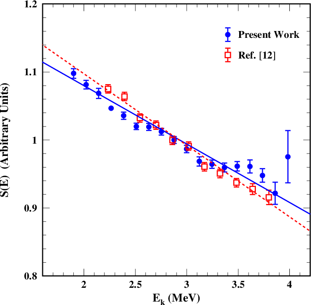
Recall that in our experiment, we determine only ratios of the values at different currents and that we have fixed the value of at 11 A. In the plot to follow, the corresponding value is shown without an error bar. The uncertainties shown for the remaining data points are effective 1 Poisson errors, obtained by locating the points in parameter space where is smaller than the maximum value by 0.5. Because we measure ratios and ratios of ratios, the uncertainties in the values are strongly correlated.
Our results are presented in Fig. 11. Here we plot the ratio of the extracted spectrum, , to the allowed statistical shape:
| (10) |
where is the positron energy, is the endpoint energy corrected for nuclear recoil (4.63223 MeV), and is the usual Fermi function for a point charge nucleus with lepton wave functions evaluated at the nuclear surface (see for example Ref. [22]). The data set has been normalized to at roughly the center of the measured energy range. For comparison we also show the previous measurements of this quantity reported by SG [12], normalized in the same way. We see that the two data sets are similar, although the new measurements have a somewhat smaller slope than the previous ones. Also, the new measurements extend over a larger energy range.
Besides the points shown in Fig. 11 we have measurements at both 18.5 and 19.0 A. Determination of at the highest currents is complicated by the low counting rates for real positrons and by the proximity to the endpoint which leads to large corrections for the finite acceptance of the spectrometer. At 18.5 A, where the kinetic energy at the centroid of the acceptance function is only 10 keV below the endpoint, we observe a total of 208 counts with an expected background of 179. After applying the finite acceptance correction factor of 3.7, the resulting measurement is in agreement with the trend of the data shown in Fig. 11. Our highest current (19 A) is above the 14O endpoint. There we have 101 observed counts with an expected background of 104. These high-current results give us confidence that our treatment of the backgrounds and the finite acceptance correction are adequate.
VI Determination of the Shape Parameters
Before extracting detailed shape information from our data, we want to account for all the energy dependences that are known to be present for purely allowed transitions. For this purpose we define a modified Fermi function
| (11) |
Here is a radiative correction factor calculated following Sirlin [21], and are finite size corrections as given by Wilkinson [22], and and are corrections for recoil and screening, respectively, again calculated according to Wilkinson [23].
We then construct a shape function with this modified Fermi function:
| (12) |
Most of the correction factors that appear in Eq. (11) are quite close to 1, the exception being the radiative correction term. That factor has a negative slope and varies by about 2% over the range of our measurements. Consequently, the plot of looks much like in Fig. 11 except with a slightly reduced slope.
Based on past theoretical work (see Sec. II), we expect that contributions from terms beyond and are not negligible, and therefore it is not appropriate to fit our measurements with a function of the form given in Eq. (3). Instead we exploit the observation by Behrens and Bühring (see Ref. [24], page 462) that the shape function for allowed transitions can be written in the form
| (13) |
where is the positron total energy in units of its rest energy, and where and the shape parameters , and are all constants.

Since we have measurements of over a limited energy range, it is completely impractical to determine all three shape parameters, and so to develop a fitting strategy, we turn to the theoretical calculations for guidance. Towner and Hardy [14] tabulate the shape parameters for a variety of shell model wave functions, while García and Brown [13] provide enough information to allow these quantities to be computed. All the calculations we have seen suggest that the term is very small over our energy range. In addition, the and terms are strongly correlated in such a way that a change in the value of can be compensated by a much smaller change in . Finally, since the calculated ’s all tend to be of about the same size, we will fix this parameter at a typical theoretical value.
If one fits measurements with and , one learns that these two parameters are also strongly correlated. The term allows for curvature in , but if this term becomes substantial, it contributes to the overall slope. In this way, uncertainty in the curvature translates into an uncertainty in . To get around this difficulty, we fit the data with an algebraically equivalent formula,
| (14) |
where is taken to be the value corresponding to a kinetic energy of 2.75 MeV, close to the middle of our measured energy range. With this choice the term has zero slope at , virtually eliminating the correlation between and .
The fitting procedure basically follows the method outlined in Sec. V.3. Given , and , we compute from Eq. (7) and then fit the measured sums via Eq. (6) by maximizing the Poisson likelihood function. With fixed at 0.04 we obtain the central result of the present work:
| (15) |
In Eq. (15) the quoted uncertainties are once again the effective 1 statistical Poisson errors. The quality of the fit is good. A detailed statistical analysis indicates that for the current problem one should expect best fit values in the range , and our result is .
Given the primed shape parameters it is straightforward to calculate the unprimed ones. The result is , , and . Our fixed value for was chosen to give in agreement with typical theoretical predictions (see for example Ref. [14] Table III).
The best fit is shown in Fig. 12, along with our experimental results for . The agreement between the curve and the experimental points seems to be good, though we need to remember that the experimental uncertainties are strongly correlated. Nevertheless, it is clear from the plot that the measurements favor a fit with a positive curvature.
VI.1 Systematic Errors
There are several non-trivial sources of systematic error in the shape parameters. We use measured 66Ga spectra and Monte-Carlo calculations to correct for positron events that fall below the threshold of our Si(Li) summation window. The 66Ga measurements have statistical uncertainties, and we also found it necessary to renormalize the Monte-Carlo spectra in the region below channel 40. We estimate that the combined uncertainties associated with the sub-threshold corrections are and .
The spectrometer is calibrated to an accuracy of 1 part in leading to an uncertainty in the central momentum of the detected positrons. The resulting systematic error contributions are and . We apply corrections for flux pinning in the superconducting magnets [17]. Taking the uncertainty to be half the correction gives and .
We subtract counts that result from 2.3 MeV -rays, but there are possible systematic errors in the required Monte-Carlo simulations. We estimate the resulting systematic uncertainties to be and . Uncertainties arising from the other background sources are small, and . The uncertainties associated with backscattering from the aluminum source foil are similarly small, and .
Besides the error sources listed above, we have also considered systematic errors arising from the uncertainties in the -decay value and lifetime, from deadtime and pileup, and from the uncertainty in the spectrometer acceptance width (see Ref. [20]). All of the resulting systematic error estimates are negligible.
Combining all of the systematic uncertainties in quadrature, we obtain net systematic errors of
| (16) |
VII Discussion
Let us compare our shape parameters with those obtained from the measurements of SG [12]. For this purpose we use the values and uncertainties given in Table 1 of TH [14]. We fit these data with the formula given in Eq. (14), taking , and as free parameters and fixing at 0.04. The results are
| (17) |
As we expect from Fig. 11, the SG data have a greater slope than the new measurements. Somewhat unexpected is the fact that the SG data also favor a positive curvature, statistically consistent with our result. One can possibly see a slight curvature in data of Fig. 11, but that curvature is enhanced by the correction factors which are applied to convert to .
The central question is whether the new measurements are consistent with CVC. In the naive picture in which GT and WM are the only non-zero matrix elements, should be of the form Eq. (1) with
| (18) |
provided that CVC and charge symmetry hold. This conclusion is correct whether or not one renormalizes the GT and M1 (or equivalently WM) operators as described in Ref. [14]. Our measurements have a greater slope than one obtains from Eq. (18), and as we have emphasized, the measurements also have a non-zero curvature which is inconsistent with Eq. (1) no matter what the value of . Therefore, higher order terms are clearly required.
At this point it is helpful to turn to detailed shell model calculations. Towner and Hardy [14] have reported shape parameters for a number of such calculations. These authors begin with shell model wave functions from various sources and then allow mixing between the first and second eigenvectors of the calculation, by fitting the measurements of SG. This is almost the same as fitting the value. When the authors use free particle operators, the best fit theoretical has about the right slope, but the resulting values are not consistent with CVC and the known M1 electromagnetic decay. The calculations are then repeated with renormalized GT and WM operators, and in this case the values are within 10% of the CVC value.
Results obtained with renormalized operators are given in Table III of TH [14]. These calculations [25] all have values in the range to , covering our measured value. The “CK” calculation, for which matches the CVC prediction to better than %, gives .
More can be learned from García and Brown [13]. In Table VIII GB report values of 5 matrix elements, , , , and . is a linear combination of and ,
| (19) |
and the authors choose to satisfy CVC. The value of , which is our , is chosen to reproduce the measured value. We know that the shape parameters are very sensitive to variations in , and therefore we re-optimize this parameter to obtain a decay constant for the transition of /s. This result corresponds to a ground-state branching ratio of 0.54% obtained by TH in their reanalysis of the SG data set.
We take numerical values for the matrix elements from Table VIII of GB, and after making the small adjustment in we compute the shape parameters. The resulting values for the three shell model wave functions considered by GB fall in the range to .

Many of the results quoted above are summarized in Fig. 13. In panel (a) we show our measured value of along with the result we extract from the SG data. The points shown without error bars are the TH and GB calculations discussed above, and as we can see, the theoretical points cluster around our measured value.
The agreement between theory and experiment for the curvature parameter is not so good. In panel (b) of Fig. 13 we see theoretical values ranging from 0.0010 to 0.0025, several standard deviations from the measured value of 0.0061.
To understand what all of this means we would like to know how various matrix elements affect the calculated shape parameters. Suppose we start from one of the GB calculations and arbitrarily change from the CVC value by 10% by shifting either or . The result we find is that shifts by 8% (0.0021) while moves by only . We conclude that the discrepancy between our measured curvature and the theoretical predictions has nothing to do with CVC.
We can also investigate what happens when we shift values of the higher order matrix elements and . For both of these we find that a shift in the matrix element value moves and by similar amounts. In view of this, it seems plausible that with the right values of and , one might improve the agreement with without seriously degrading the present slope parameter agreement.
Overall, we are very pleased with the results. We have seen that the slope parameter is very sensitive to the value of , and the agreement of our measured value with calculations that respect CVC is excellent. The lack of similarly close agreement with the measured curvature parameter should probably not be a major concern. In fact, if we add the statistical and systematic uncertainties, the largest theoretical values are less than 2 standard deviations from the measured value.
All of the theoretical curves actually reproduce the new measurements fairly well. This is illustrated in Fig. 12 where the shaded band shows the range of predictions covered by the three calculations listed in Table III of TH. Since we have not reported a measurement of the absolute magnitude of , we renormalize the TH curves to match the scale of the plotted points. Given that these calculations were originally optimized in an effort to reproduce the SG data, the agreement with the present measurements is remarkably good. The calculations of GB would produce a similar, but slightly wider, band.
VIII Summary
We have carried out an experiment designed to test CVC by measuring the shape of the -spectrum for the decay of 14O to the ground state of 14N. The measured shape function has a slope somewhat smaller in magnitude than that of the measurements reported in Ref. [12]. The new measurements allow us to determine the value of a parameter, , which is essentially the average slope of the shape function over the energy range of our measurements, to a relative accuracy of better than 3%.
The measured slope parameter is in good agreement with predictions from theoretical calculations that respect CVC by requiring agreement between the -decay weak magnetism matrix element, , and the M1 matrix element for the electromagnetic decay of the first excited state of 14N.
The authors wish to thank Alejandro García for suggesting the experiment. We also thank Laura Kinnaman, Megan McGowan and Li Zhan for their assistance on the project, and the University of Wisconsin Center for High Throughput Computing for allowing access to their computational facilities. This work was supported in part by the National Science Foundation under grants Nos. PHY-0855514 and PHY-0555649, and in part by an allocation of time from the Ohio Supercomputer Center.
References
- [1] A.T. Laffoley, et al., Phys. Rev. C 88, 015501 (2013).
- [2] D.R. Inglis, Rev. Mod. Phys. 25, 390 (1953).
- [3] W.M. Visscher and R.A. Ferrell, Phys. Rev. 107, 781 (1957).
- [4] F.P. Calaprice and B.R. Holstein, Nucl. Phys. A273, 301 (1976).
- [5] M. Gell-Mann, Phys. Rev. 111, 362 (1958). (1957).
- [6] R.P. Feynmann and M. Gell-Mann, Phys. Rev. 109, 193 (1957).
- [7] T. Mayer-Kukuk and T.C. Michel, Phys. Rev. 127, 545 (1962).
- [8] C.S. Wu, Y.K. Lee, and L.W. Mo, Phys. Rev. Lett. 39, 72 (1977).
- [9] W. Kaina, V. Soergel, H. Thies, and N. Trost, Phys. Lett. 70B, 411 (1977).
- [10] J.B. Camp, Phys. Rev. C 41, 1719 (1990).
- [11] L. Grenacs, Ann. Rev. Nucl. Part. Sci. 35, 455 (1985).
- [12] G.S. Sidhu and J.B. Gerhart, Phys. Rev. 148, 1024 (1966).
- [13] A. García and B.A. Brown, Phys. Rev. C 52, 3416 (1995).
- [14] I.S. Towner and J.C. Hardy, Phys. Rev. C 72, 055501 (2005).
- [15] S. Raman, C.A. Houser, T.A. Walkiewicz, and I.S. Towner, At. Data Nucl. Data Tables 21, 567 (1978).
- [16] I.S. Towner and F.C. Khanna, Nucl. Phys. A399, 334 (1983).
- [17] L.D. Knutson, G.W. Severin, S.L. Cotter, L. Zhan, P.A. Voytas and E.A. George, Rev. Sci. Instrum. 82, 073302-1, (2011).
- [18] David E. Alburger, Rev. Sci. Instrum. 27, 991 (1956).
- [19] I. Kawarakow, E. Mainegra-hing, D.W.O. Rogers, F. Tessier and B.R.B. Walters, NRCC Report PIRS-701 (2011).
- [20] G.W. Severin, L.D. Knutson, P.A. Voytas and E.A. George, Phys. Rev. C 89, 057302 (2014).
- [21] A. Sirlin, Phys. Rev. 164, 1767 (1967).
- [22] D.H. Wilkinson, Nucl. Instrum. Meth. A290, 509 (1990).
- [23] D.H. Wilkinson, Nucl. Instrum. Meth. A335, 182 (1993).
- [24] H. Behrens and W. Bühring, Electron Radial Wave Functions and Nuclear Beta Decay (Oxford University Press, New York, 1982).
- [25] I.S. Towner and J.C. Hardy, private communication. The authors fit their numerical calculations with an expression of the form . To obtain and we refit the curve with Eq. (14) keeping fixed at 0.04.