Heteroscedastic Treed Bayesian Optimisation
John-Alexander M. Assael Ziyu Wang Bobak Shahriari Nando de Freitas Imperial College London University of Oxford University of British Columbia University of Oxford CIFAR Fellow
Abstract
Optimising black-box functions is important in many disciplines, such as tuning machine learning models, robotics, finance and mining exploration. Bayesian optimisation is a state-of-the-art technique for the global optimisation of black-box functions which are expensive to evaluate. At the core of this approach is a Gaussian process prior that captures our belief about the distribution over functions. However, in many cases a single Gaussian process is not flexible enough to capture non-stationarity in the objective function. Consequently, heteroscedasticity negatively affects performance of traditional Bayesian methods. In this paper, we propose a novel prior model with hierarchical parameter learning that tackles the problem of non-stationarity in Bayesian optimisation. Our results demonstrate substantial improvements in a wide range of applications, including automatic machine learning and mining exploration.
1 Introduction
Bayesian optimisation has proven to be a popular and successful methodology for global optimisation of expensive, black-box functions. It is used to find the global minimum of generally non-convex, multi-modal functions whose derivatives are unavailable. The evaluations of the objective function are often only available via noisy observations. Major applications of these techniques include interactive user interfaces (Brochu et al., 2010) robotics (Lizotte, 2008; Martinez–Cantin et al., 2009), environmental monitoring (Marchant and Ramos, 2012), estimating thermophysical properties of materials (Assael et al., 2014), information extraction (Wang and de Freitas, 2014), sensor networks (Garnett et al., 2010; Srinivas et al., 2010), adaptive Monte Carlo (Wang et al., 2013), experimental design (Azimi et al., 2012), and reinforcement learning (Brochu et al., 2009). An application that has inspired great interest recently is that of automatically tuning machine learning algorithms (Hutter et al., 2011a; Bergstra et al., 2011; Snoek et al., 2012; Swersky et al., 2013; Thornton et al., 2013; Hoffman et al., 2014).
In general, the goal of global optimisation is to find the optimum
| (1) |
of an objective function over an index set . The approach of Bayesian optimisation may be understood in the setting of sequential decision making, whereby at the -th decision round, we select an input and observe the value of the black-box reward function . The returned value may be deterministic, , or stochastic, , where is a noise process.
Since the function is unknown, we use a Bayesian prior model to encode our beliefs about its smoothness, and an observation model to describe the data up to the -th round. Using these two models and the rules of probability, we derive a posterior distribution that can in turn be used to build an acquisition function to decide the next input query . The acquisition function trades-off exploitation and exploration in the search process. For a comprehensive introduction of Bayesian optimisation, please refer to (Brochu et al., 2009; Snoek et al., 2012).
Most of the aforementioned practical applications tend to have heteroscedastic objective functions. Snoek et al. (2013) addressed this fundamental problem using warped Gaussian processes. In this work, we introduce a flexible novel model for dealing with heteroscedasticity. In particular, we adopt trees with (warped) Gaussian process leaves. We explain how to construct these trees properly avoiding variance explosion near split points. We also introduce a hierarchical approach for learning the hyper-parameters, so as to address situations in which only a few points are observed at each leaf. All these methodological improvements, where combined resulting significantly improved empirical performance in a wide range of applications.
2 Background
In this section, we give a brief overview of Bayesian optimisation as well as a brief survey on Heteroscedastic Gaussian processes.
2.1 Gaussian processes
Gaussian processes (GPs) are popular priors for Bayesian optimisation as they offer a simple and flexible model to capture our beliefs about the behaviour of the function; we refer the reader to Rasmussen and Williams (2006) for details on these stochastic processes. These priors are defined by a mean function and a covariance kernel . Given any collection of inputs , the outputs are jointly Gaussian:
where denotes the vector of prior mean evaluated at the data, i.e. ; and is the covariance matrix between observed data points, parameterised by . For convenience, in this work we use a constant prior mean function.
The choice of covariance function is important as it governs the smoothness of the function. While squared exponential kernels are popular, we opt for the Matérn(5/2) kernel with automatic relevance determination:
| (2) |
where and is the diagonal matrix of squared length scale parameters . Let denote the hyper-parameters which completely characterize our kernel. The Matérn(5/2) makes less stringent smoothness assumptions than the squared exponential kernel and is thus a better fit for heteroscedastic Bayesian optimisation.
Given the noise-corrupted observations , the joint distribution of these observations and an arbitrary point is:
where and . By conditioning on the observed , the posterior predictive distribution of an arbitrary point is marginally Gaussian with mean and variance
| (3) | ||||
| (4) |
respectively.
2.2 Acquisition functions
Having specified a distribution to capture our beliefs about the behaviour of the function, as well as a mechanism to update it at each step, we define an acquisition function for choosing the next evaluation point
The acquisition function must trade-off exploration and exploitation to ensure that the location of the global maximum (or minimum) is found in as few steps as possible.
Although many acquisition strategies have been proposed (see for example Močkus (1982); Jones (2001); Hoffman et al. (2011); Hennig and Schuler (2012); Snoek et al. (2012); Hoffman et al. (2014); Wang et al. (2014a); Shahriari et al. (2014)), the expected improvement (EI) criterion remains a default choice in popular Bayesian optimisation software packages, such as SMAC and Spearmint (Hutter et al., 2011b; Snoek et al., 2012). If we let
denote the current incumbent, the EI acquisition function can be written in closed form as
with
and , representing the standard normal density and distribution functions respectively. In the special case of , we set . The expected improvement is best understood as a family of one-step-decision heuristics Brochu et al. (2009), with many members in this family.
2.3 Related work
Several approaches have been proposed to manage heteroscedasticity with Gaussian processes. Sampson and Guttorp (1992) attempted to project inputs into a latent space that is stationary. This approach was later extended by Schmidt and O’Hagan (2003). A latent space representation in higher dimensions was also proposed by Bornn et al. (2012). Others such as Higdon et al. (1999) and Williams and Rasmussen (2006) have tried to model heteroscedasticity directly with the choice of covariance function. In 2005, Gramacy proposed a treed GP model to attack non-stationarity. While this work, as well as, the work of Dunson and Fox (2012), are the closest to ours, both were developed for modelling functions and not for global optimisation under a limited number of observations.
Warping is another popular approach for dealing with non-stationarity (Snelson et al., 2004; Adams and Stegle, 2008). Recently, Snoek et al. (2013) proposed an input warping technique, using a parameterised Beta cumulative distribution function (CDF) as the warping function. The goal of input warping is to transform non-stationary functions to stationary ones by applying a Beta CDF mapping to each dimension . The new covariance becomes . We have found that input warping can lead to remarkable improvements in automatic algorithm configuration. However, the Beta CDF transformation has limitations, which we address in this paper by using a treed approach.


3 Treed Bayesian Optimisation
3.1 Constructing the tree structure
Our proposed heteroscedastic treed Bayesian optimisation (HTBO) method is based on classification and regression trees (CART), a decision tree model of Breiman et al. (1984). A Decision tree may be understood in terms of a sequence of binary tests applied to an input , which determines the path followed by from the root of the tree to a leaf. Each node has a function of the form , where extracts a coordinate (feature) of and compares it to a threshold . The tree is constructed in a recursive manner by choosing splits on features and thresholds so as to reduce uncertainty (Denil et al., 2014).
We can measure uncertainty in a node using the empirical mean squared error:
where is the average of the output values in . We could also use the entropy of the GPs in each node, but we found this alternative uncertainty measure to require much more computation without leading to better performance.
The optimal splits on features and thresholds are the ones that reduce uncertainty the most when splitting node into and . They are obtained by optimising the following reduction in uncertainty objective:
| (5) |
In CART, the splitting threshold of feature is the midpoint of two points , which is convenient for constant predictions as will go to the left child and to the right one respectively. However, in the proposed approach this would create unwanted variance in the gap between and , as one GP will have to cover the unknown space from to and another GP the unknown space from to . This antagonises the goal of minimising the conditional variance in Bayesian Optimisation (Brochu et al., 2007) as shown in the left plot of Figure 2.
We solve the problem of the unwanted variance, by placing exactly at one of the points , and let belong to both children nodes, as shown on the right hand side of Figure 2. This splitting strategy is essential for Bayesian optimisation to work well with treed GPs.
3.2 Learning hyper-parameters
Whereas other treed GP models propose partitioning the data for computational efficiency (Gramacy et al., 2004; Bui and Turner, 2014) or capturing multiple scales in the data (Dunson and Fox, 2012), our approach is designed to learn non-stationarity in the random process that generated the objective function. Therefore, it is paramount that our model is capable of learning different hyper-parameters for each leaf.
Maximum likelihood is a common technique for obtaining a point estimate of the hyper-parameters. In GP regression, the log-marginal-likelihood can be expressed analytically as follows
| (6) |
A straightforward implementation of this approach for our purpose would independently maximise the log-marginal-likelihood of the data in each leaf. When leaves have very few data points, however, maximising the likelihood could severely underestimate the length scale hyper-parameters.
In this section, we propose a way of aggregating information from different levels of the tree hierarchy. Given a tree-structured partition of current observations constructed as per the previous section, let nodes be integer indexed, starting with the root node . Let denote the data in node and denote the data in node excluding the data in node , and similarly for and . Furthermore, let return the depth of node such that and let return the ordered list of nodes in the path from the node to the root , such that and , and finally let denote the set of leaves of the tree.
Suppose we are interested in estimating the hyper-parameters of the GP associated with leaf , consider the following marginal pseudo-likelihood decomposition
| (7) |
This decomposition implicitly assumes certain conditional independencies between nodes in the tree, given . Each factor corresponds to a node along the path of the leaf in question. However, the factors are all equally weighted, so that the estimated hyper-parameter fits all of the data equally. Consider instead, for each leaf , a weighted marginal pseudo-likelihood decomposition
| (8) |
where the importance of each factor depends on its corresponding node’s depth relative to leaf . A simple example of this factor decomposition is depicted in Figure 3.
The weighted likelihood was inspired by the work of (Newton and Raftery, 1994) and paves us the way to produce samples from the posterior of interest. Finally, the weights are selected so that the factor corresponding to the leaf is squared and weights decrease harmonically along the path :
| (9) |
So far, for ease of presentation, we have focused our attention on maximising the marginal likelihood (also known as empirical Bayes or maximum likelihood II). However, it is straightforward to adopt a more Bayesian approach by prescribing a prior and inferring the hyper-parameters of leaf by targeting the following unnormalised posterior
| (10) |
using Markov chain Monte Carlo (MCMC).
3.3 Heteroscedastic treed Bayesian optimisation
At each iteration of Bayesian optimisation, the decision tree is reconstructed. In doing so, we ensure that there is a minimum number of data points per leaf (5 in our experiments). Subsequently, we estimate the hyper-parameters as discussed in the previous section. The same approach is also used in the estimation of the mean and the kernel amplitude of the GP. Once the GPs have been fit to the data in each leaf, we use their statistics to construct the EI acquisition function. This function is then optimised using a -dimensional Sobol Grid with points as in the package Spearmint.
It is interesting to note that, HTBO does not place explicit requirements on the GP leaves, so long as, we can compute the log-marginal-likelihood and EI efficiently. As a result, not only could we use standard GPs but also GPs with warping (Snoek et al., 2013) as leaves. When employing warping, the and parameters of the Beta CDF are estimated using the proposed hierarchical prior. We refer to HTBO with Warping as HTBO Warp and evaluate it in our experiments.
Example iterations of the proposed treed approach against standard Bayesian optimisation on a one-dimensional heteroscedastic function are illustrated in Figure 1. While the standard approach fails, the proposed method, hierarchical treed Bayesian optimisation (HTBO), is able to overcome non-stationarity to find the maximum of the objective function.
4 Experiments
In this section we evaluate the proposed methods HTBO and HTBO Warp. Comparisons are made against standard Bayesian optimisation (BO), as well as, the Bayesian optimisation approach with input warping (BO Warp) of (Snoek et al., 2013). For all the experiments presented in this paper, we used the Matérn(5/2) kernel. The GP hyper-parameters of all four approaches are obtained using slice sampling. We use three different sets of experiments for evaluation: synthetic functions, algorithm configuration benchmarks, and mineral exploration datasets. The results are summarised and discussed in Section 4.4.
4.1 Synthetic problems
We first introduce two heteroscedastic synthetic functions. The first synthetic function, which we refer to as RKHS, is shown in Figure 1. The function is constructed as a weighted sum of squared exponential kernel functions with 2 different length scales. The left hand side of the function is smooth, whereas the right hand size jagged. For a more detailed description, as well as, the source code of the function, please refer to Wang et al. (2014b).
The second synthetic function is a two-dimensional exponential function from Gramacy (2005). The precise mathematical expression for the function is:
| (11) |
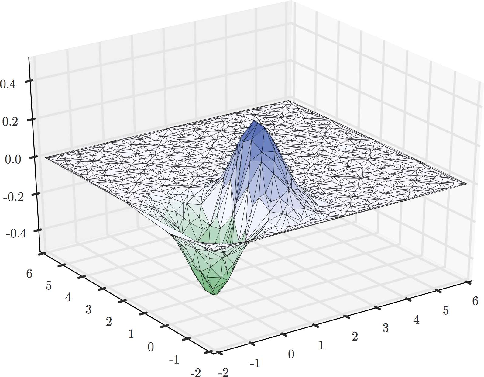
We refer to this function as 2-D Exp. and plot it in Figure 4. This function is interesting because it is “flat” over most of its domain, with a peak that can be easily missed without careful exploration.
4.2 Automatic machine learning problems
Latent Dirichlet Allocation (LDA) is a directed graphical model for documents used in topic modelling tasks, for which Hoffman et al. (2010) proposed an online learning approach in the variational Bayes paradigm. In this experiment we use precomputed performance data for this on-line LDA algorithm on a dataset of 250,000 Wikipedia articles under many parameter settings. Tuning the online LDA algorithm involves choosing the two learning parameters, and as well as a third parameter specifying the mini-batch size, yielding a three-dimensional problem. Following the original authors, the search space is restricted to a grid (Hoffman et al., 2010). Next, we optimize a latent structured support vector machine (SVM) using a dataset available from Snoek et al. (2012). Similarly to the LDA tuning experiment, the authors consider the latent structured SVM on a three-dimensional parameter settings space of two regularisation parameters and a convergence tolerance. We used precomputed data corresponding to the performance of the algorithm on binary classification of protein DNA sequences. Once again following the original methodology, the three-dimensional search space is discretised in a grid (Yu and Joachims, 2009; Miller et al., 2012).
Both datasets serve as benchmarks in the algorithm configuration community and the performance of a few different global optimisation approaches on these datasets is publicly available from Eggensperger et al. (2013).
| Method | BO | BO Warp | HTBO | HTBO Warp |
|---|---|---|---|---|
| RKHS | ||||
| 2-D Exp | ||||
| LDA | ||||
| SVM | ||||
| Agromet | ||||
| Brenda |
4.3 Geostatistical problems
In geostatistics, Kriging is a method of interpolation with the aim of modelling a function efficiently with a minimal number of observations. Hence, Kriging is very closely related to Bayesian Optimisation. In this subsection, we describe two datasets available at kriging.com.

The Agromet dataset was acquired by Isobel Clark, and describes a square area in the Natal Highlands, South Africa, measuring Gold grade of a drill hole intersection at -meter spacing. Hence, this example is two-dimensional and is defined by the latitude and the longitude values of each acquired sample. There are in total 18,189 observations. As shown in Figure 6, the surface described by the dataset is clearly heteroscedastic and very rough, making it difficult for a single Gaussian process, even with input warping, to model accurately.
Brenda is an dataset of 1,856 observations of the depths of a copper mine in British Columbia, Canada, that was closed in 1990. Each observation in the dataset measures the concentrations of Copper, Molybdenum, Silver and Gold deposits. As in the case of Agromet, the surface described by Brenda also exhibits non-stationarity. In our experiments, we try only to identify the areas that contain the highest concentrations of Copper.
Please refer to Clark and Harper (2008) for more comprehensive descriptions of these datasets. In this paper, we use these two Kriging examples to construct optimisation problems by trying to find the highest concentrations of ores, based on the physically observed values of the datasets. Hence, we only query the expected improvement function at the points available from the historical records.
4.4 Evaluation
Each of the approaches was run times on all of the six benchmarks. Figure 5 summarises the average performance of all the runs. In all examples, we try to minimize (instead of maximise) the objective function to follow the convention of earlier work Snoek et al. (2012); Snoek et al. (2013). We also report the mean and standard deviation of the runs in Table 1.
In the experiment involving the RKHS function (Figure 5 (a)), most of the BO and BO Warp runs failed to converge to the global optimum. In contrast, by taking advantage of the tree partitioning, the proposed HTBO and HTBO Warp approaches are capable of modelling and optimising the heteroscedastic objective function, with the latter achieving optimal performance. Specifically, HTBO Warp converged to the global optimum of the function in approximately evaluations. As illustrated in Figure 5 (b), BO Warp performs inadequately on the 2D Exp. function, while HTBO and HTBO Warp exhibit the fastest convergence. This illustrates the fact that input warping, despite being a very powerful technique, can fail in some heteroscedastic domains.
On the problem of online LDA, as shown in Figure 5 (c), the best performance was achieved by HTBO and HTBO Warp, with BO Warp following closely. On the structured SVM example, in Figure 5 (d), all methods have similar performance. It appears that both problems are simple enough that all four methods converge eventually. It is important to note that despite the lack of significant heteroscedasticity, the proposed methods are still competitive with the state of art.
Finally, in the two real-world mining extraction problems HTBO and HTBO Warp achieve a significantly faster rate of convergence. They outperform BO and BO Warp, that can’t efficiently deal with the high heteroscedasticity of the domain. The performance is depicted in more detail in Figures 5 (e-f).
5 Conclusion
In this work, we introduced HTBO, a model based on decision trees with GP leaves, for tackling hard heteroscedastic functions in Bayesian optimisation. HTBO is a flexible model that does not place explicit requirements on its GP leaves and it can readily be combined with input warping (HTBO Warp). We proposed a weighted marginal likelihood approach for learning the hyper-parameters of the leaves, and demonstrated empirically that our proposed methodological improvements have robust behaviour across a wide range of heteroscedastic functions. Finally, after evaluating the performance of HTBO and HTBO Warp on six problems, we showed that the proposed approaches outperform the competition in normal and heteroscedastic settings, and can yield both performance gains and robustness.
References
- Adams and Stegle (2008) Adams, R. P. and Stegle, O. (2008). Gaussian process product models for nonparametric nonstationarity. In ICML, pages 1–8.
- Assael et al. (2014) Assael, M., Antoniadis, K., Metaxa, I., Mylona, S., Matziaroglou, G., Efopoulos, V., Assael, J.-A., Marini, K., Wu, J., and Hu, M. (2014). A novel portable absolute two-wires transient hot-wire instrument for the measurement of the thermal conductivity of solids. In 20th European Conference on Thermophysical Properties.
- Azimi et al. (2012) Azimi, J., Jalali, A., and Zhang-Fern, X. (2012). Hybrid batch Bayesian optimization. In ICML.
- Bergstra et al. (2011) Bergstra, J., Bardenet, R., Bengio, Y., and Kégl, B. (2011). Algorithms for hyper-parameter optimization. In NIPS, pages 2546–2554.
- Bornn et al. (2012) Bornn, L., Shaddick, G., and Zidek, J. V. (2012). Modeling nonstationary processes through dimension expansion. Journal of the American Statistical Association, 107(497), 281–289.
- Breiman et al. (1984) Breiman, L., Friedman, J., Stone, C. J., and Olshen, R. A. (1984). Classification and regression trees. CRC press.
- Brochu et al. (2007) Brochu, E., de Freitas, N., and Ghosh, A. (2007). Active preference learning with discrete choice data. In NIPS, pages 409–416.
- Brochu et al. (2009) Brochu, E., Cora, V. M., and de Freitas, N. (2009). A tutorial on Bayesian optimization of expensive cost functions, with application to active user modeling and hierarchical reinforcement learning. Technical Report UBC TR-2009-23 and arXiv:1012.2599v1, Dept. of Computer Science, University of British Columbia.
- Brochu et al. (2010) Brochu, E., Brochu, T., and de Freitas, N. (2010). A Bayesian interactive optimization approach to procedural animation design. In ACM SIGGRAPH / Eurographics SCA, pages 103–112.
- Bui and Turner (2014) Bui, T. D. and Turner, R. E. (2014). Tree-structured Gaussian process approximations. In Advances in Neural Information Processing Systems, pages 2213–2221.
- Clark and Harper (2008) Clark, I. and Harper, W. V. (2008). Practical Geostatistics 2000: Case Studies. Ecosse North America.
- Denil et al. (2014) Denil, M., Matheson, D., and de Freitas, N. (2014). Narrowing the gap: Random forests in theory and in practice. In ICML.
- Dunson and Fox (2012) Dunson, D. B. and Fox, E. B. (2012). Multiresolution Gaussian processes. In Advances in Neural Information Processing Systems, pages 737–745.
- Eggensperger et al. (2013) Eggensperger, K., Feurer, M., Hutter, F., Bergstra, J., Snoek, J., Hoos, H., and Leyton-Brown, K. (2013). Towards an empirical foundation for assessing Bayesian optimization of hyperparameters. In NIPS Workshop on Bayesian Optimization in Theory and Practice.
- Garnett et al. (2010) Garnett, R., Osborne, M. A., and Roberts, S. J. (2010). Bayesian optimization for sensor set selection. In ACM/IEEE International Conference on Information Processing in Sensor Networks, pages 209–219. ACM.
- Gramacy (2005) Gramacy, R. B. (2005). Bayesian treed Gaussian process models. Ph.D. thesis, University Of California Santa Cruz.
- Gramacy et al. (2004) Gramacy, R. B., Lee, H. K. H., and Macready, W. G. (2004). Parameter space exploration with Gaussian process trees. In ICML, pages 45–52.
- Hennig and Schuler (2012) Hennig, P. and Schuler, C. (2012). Entropy search for information-efficient global optimization. JMLR, 13, 1809–1837.
- Higdon et al. (1999) Higdon, D., Swall, J., and Kern, J. (1999). Non-stationary spatial modeling. Bayesian statistics, 6(1), 761–768.
- Hoffman et al. (2010) Hoffman, M., Bach, F. R., and Blei, D. M. (2010). Online learning for latent Dirichlet allocation. In NIPS, pages 856–864.
- Hoffman et al. (2011) Hoffman, M., Brochu, E., and de Freitas, N. (2011). Portfolio allocation for Bayesian optimization. In UAI, pages 327–336.
- Hoffman et al. (2014) Hoffman, M., Shahriari, B., and de Freitas, N. (2014). On correlation and budget constraints in model-based bandit optimization with application to automatic machine learning. In AIStats, pages 365–374.
- Hutter et al. (2011a) Hutter, F., Hoos, H. H., and Leyton-Brown, K. (2011a). Sequential model-based optimization for general algorithm configuration. In LION, pages 507–523.
- Hutter et al. (2011b) Hutter, F., Hoos, H. H., and Leyton-Brown, K. (2011b). Sequential model-based optimization for general algorithm configuration. In LION, pages 507–523.
- Jones (2001) Jones, D. (2001). A taxonomy of global optimization methods based on response surfaces. Journal of Global Optimization, 21(4), 345–383.
- Lizotte (2008) Lizotte, D. (2008). Practical Bayesian Optimization. Ph.D. thesis, University of Alberta, Canada.
- Marchant and Ramos (2012) Marchant, R. and Ramos, F. (2012). Bayesian optimisation for intelligent environmental monitoring. In Intelligent Robots and Systems (IROS), 2012 IEEE/RSJ International Conference on, pages 2242–2249. IEEE.
- Martinez–Cantin et al. (2009) Martinez–Cantin, R., de Freitas, N., Brochu, E., Castellanos, J., and Doucet, A. (2009). A Bayesian exploration-exploitation approach for optimal online sensing and planning with a visually guided mobile robot. Autonomous Robots, 27(2), 93–103.
- Miller et al. (2012) Miller, K., Kumar, M. P., Packer, B., Goodman, D., Koller, D., et al. (2012). Max-margin min-entropy models. In AIStats.
- Močkus (1982) Močkus, J. (1982). The Bayesian approach to global optimization. Systems Modeling and Optimization, 38, 473–481.
- Newton and Raftery (1994) Newton, M. A. and Raftery, A. E. (1994). Approximate bayesian inference with the weighted likelihood bootstrap. Journal of the Royal Statistical Society. Series B (Methodological), pages 3–48.
- Rasmussen and Williams (2006) Rasmussen, C. E. and Williams, C. K. I. (2006). Gaussian Processes for Machine Learning. The MIT Press.
- Sampson and Guttorp (1992) Sampson, P. D. and Guttorp, P. (1992). Nonparametric estimation of nonstationary spatial covariance structure. Journal of the American Statistical Association, 87(417), 108–119.
- Schmidt and O’Hagan (2003) Schmidt, A. M. and O’Hagan, A. (2003). Bayesian inference for non-stationary spatial covariance structure via spatial deformations. Journal of the Royal Statistical Society: Series B (Statistical Methodology), 65(3), 743–758.
- Shahriari et al. (2014) Shahriari, B., Wang, Z., Hoffman, M. W., Bouchard-Cote, A., and de Freitas, N. (2014). An Entropy Search Portfolio for Bayesian Optimization. Technical Report arXiv:1406.4625, University of Oxford.
- Snelson et al. (2004) Snelson, E., Rasmussen, C. E., and Ghahramani, Z. (2004). Warped gaussian processes. NIPS, 16, 337–344.
- Snoek et al. (2012) Snoek, J., Larochelle, H., and Adams, R. P. (2012). Practical Bayesian optimization of machine learning algorithms. In NIPS, pages 2951–2959.
- Snoek et al. (2013) Snoek, J., Swersky, K., Zemel, R., and R.P. Adams, R. (2013). Input warping for Bayesian optimization of non-stationary functions. In NIPS Workshop on Bayesian Optimization in Theory and Practice.
- Srinivas et al. (2010) Srinivas, N., Krause, A., Kakade, S. M., and Seeger, M. (2010). Gaussian process optimization in the bandit setting: No regret and experimental design. In ICML.
- Swersky et al. (2013) Swersky, K., Snoek, J., and Adams, R. P. (2013). Multi-task Bayesian optimization. In NIPS, pages 2004–2012.
- Thornton et al. (2013) Thornton, C., Hutter, F., Hoos, H. H., and Leyton-Brown, K. (2013). Auto-WEKA: Combined selection and hyperparameter optimization of classification algorithms. pages 847–855.
- Wang and de Freitas (2014) Wang, Z. and de Freitas, N. (2014). Theoretical analysis of bayesian optimisation with unknown gaussian process hyper-parameters. Technical Report arXiv:1406.7758, University of Oxford.
- Wang et al. (2013) Wang, Z., Mohamed, S., and de Freitas, N. (2013). Adaptive Hamiltonian and Riemann manifold Monte Carlo samplers. In ICML, page 1462–1470.
- Wang et al. (2014a) Wang, Z., Shakibi, B., Jin, L., and de Freitas, N. (2014a). Bayesian multi-scale optimistic optimization. In AIStats, pages 1005–1014.
- Wang et al. (2014b) Wang, Z., Assael, J.-A., and de Freitas, N. (2014b). RKHS 1D Function for Bayesian Optimization tasks. https://github.com/iassael/function-rkhs.
- Williams and Rasmussen (2006) Williams, C. K. and Rasmussen, C. E. (2006). Gaussian processes for machine learning. the MIT Press, 2(3), 4.
- Yu and Joachims (2009) Yu, C.-N. J. and Joachims, T. (2009). Learning structural SVMs with latent variables. In ICML, pages 1169–1176. ACM.