Dynamics of a dipolar Bose-Einstein condensate in the vicinity of a superconductor
Abstract
We study the dynamics of a dipolar Bose-Einstein condensate, like for example a 52Cr or 164Dy condensate, interacting with a superconducting surface. The magnetic dipole moments of the atoms in the Bose-Einstein condensate induce eddy currents in the superconductor. The magnetic field generated by eddy currents modifies the trapping potential such that the center-of-mass oscillation frequency is shifted. We numerically solve the Gross-Pitaevskii equation for this system and compare the results with analytical approximations. We present an approximation that gives excellent agreement with the numerical results. The eddy currents give rise to anharmonic terms, which leads to the excitation of shape fluctuations of the condensate. We discuss how the strength of the excitation of such modes can be increased by exploiting resonances, and we examine the strength of the resonances as a function of the center-of-mass oscillation amplitude of the condensate. Finally, we study different orientations of the magnetic dipoles and discuss favorable conditions for the experimental observation of the eddy current effect.
pacs
34.35.+a, 03.75.Kk, 74.25.N-, 51.60.+aI Introduction
Magnetic microtraps are a versatile tool to trap and manipulate ultracold atomic gases and Bose-Einstein condensates (BEC). Such traps provide a strong confinement and can be integrated on a chip allowing the creation of specialized potentials and control of ultracold atomic gases by electronic means [1]. Also, the interaction of ultracold atomic gases with the surface of the nearby solid can be studied. However, the normal conductors that create the trapping potential at the same time also create noise radiation from current fluctuations, which limits the lifetime of the atomic cloud when it is brought close to the conductor [2, 3]. Recently, microtraps using superconductors have been realized [4, 5, 6, 7, 8, 9]. In such microtraps the noise due to current fluctuations is significantly suppressed in the relevant frequency range due to the energy gap of the superconductor. This allows lifetimes several orders of magnitudes longer than in conventional microtraps [10, 11, 12, 13]. Such superconducting microtraps allow studying fundamental interactions between BECs and superconductors and promise coupling of these two macroscopic quantum phenomena [14, 16, 15, 17, 18, 19, 20, 21, 22, 23].
A disadvantage of superconducting microtraps is the screening of the magnetic trapping fields due to the Meissner effect, which has been shown to lower the trap depth [6, 24]. However, theoretical calculations have shown that in spite of the Meissner effect distances below 1 m can be achieved with superconducting microtraps, if the edge enhancement of the currents in microstrips of rectangular cross-section is exploited [25, 26, 27]. A recent experiment has demonstrated a magnetic microtrap at a distance of 14 m from a superconductor [21].
In the present work we study the interaction between a dipolar Bose-Einstein condensate [28] and a superconducting surface. Dipolar BECs consist of atoms which carry a large magnetic dipole moment. The first experimental realization of a dipolar BEC succeeded with 52Cr [29]. Recently also the condensation of atoms with even larger dipole moments, like 168Er [30] or 164Dy [31] was reported. Theses systems can be used to study a number of different properties [32, 33]. In the present work we consider center-of-mass oscillations of a dipolar BEC perpendicular to a superconducting surface. The magnetic field, generated by the dipoles, induces eddy currents in the superconducting surface. The eddy currents generate a magnetic field, which in turn influences the BEC. This back action on the BEC causes a shift of the center-of-mass oscillation frequency relative to the case without a superconducting surface. In a previous work [34] we have shown that this eddy current effect generates a frequency shift which can be large enough to be detected experimentally. The characteristic dependence of the frequency shift as a function of the number of atoms in the BEC provides a fingerprint which allows to identify this eddy current effect and separate it from other surface effects like the Casimir-Polder force [35, 36], for example. We calculated the frequency shift using a relatively simple column density model for the BEC, which allowed us to find an analytical approximation. Furthermore the anharmonicity generated by the BEC-surface potential leads to a coupling of the center-of-mass motion to other collective modes of the BEC.
In our previous work we have made several simplifications: we have neglected the influence of the dipole-dipole interaction on the dynamics of the BEC, we used an effective anharmonic potential to emulate the effect of the superconducting surface, and we considered only small amplitude oscillations of the condensate. In the present work we will present a more complete and accurate investigation of the effect. We use a more realistic model by numerically solving the Gross-Pitaevskii equation (GPE) for a dipolar BEC and including the full potential generated by the surface. We will show that our previous results remain qualitatively unchanged with some quantitative corrections. Furthermore, we will consider larger amplitude oscillations. In addition, we study different polarization directions of the condensate and find another characteristic feature which can be used to experimentally identify the eddy current effect. In addition to the resonant excitation of the breather mode, on which we reported in [34], we find the resonant excitation of a different collective mode, which did not appear in our previously used effective model.
II Numerical solution of the Gross-Pitaevskii Equation for a dipolar BEC close to a superconducting surface
II.1 Modeling the system and the numerical approach
II.1.1 The Gross-Pitaevskii equation of a dipolar BEC close to a superconducting surface
Here we present the investigated system and explain the model that we use for our calculations. We consider a dilute gas of Bose atoms trapped in a harmonic potential. The potential can be generated by optical or magnetic means. For the setup under consideration, a superconducting microtrap might be the most convenient choice. The temperature of the gas shall be cooled far below the transition temperature where Bose-Einstein condensation occurs and we assume that the temperature of the gas is . This means that all the atoms in the trap will be in the condensate. Every atom carries a magnetic dipole moment . The dipoles are all aligned in the direction of an external magnetic field. The many body Hamiltonian for this Bose gas reads
| (1) |
where is the interaction potential between two atoms. The atoms can interact via short ranged -wave interaction
| (2) |
and via long ranged dipole-dipole interaction
| (3) |
where is the normalized distance vector, and are the magnetic dipole moments of the two interacting dipoles. The external trapping potential is given by
| (4) |
where is the atom mass and , and are the trapping frequencies. With the Hartree ansatz for the many body wave function
| (5) |
the energy functional can be minimized with respect to under the constraint , which then yields the Gross-Pitaevskii equation [38, 37]
| (6) | |||||
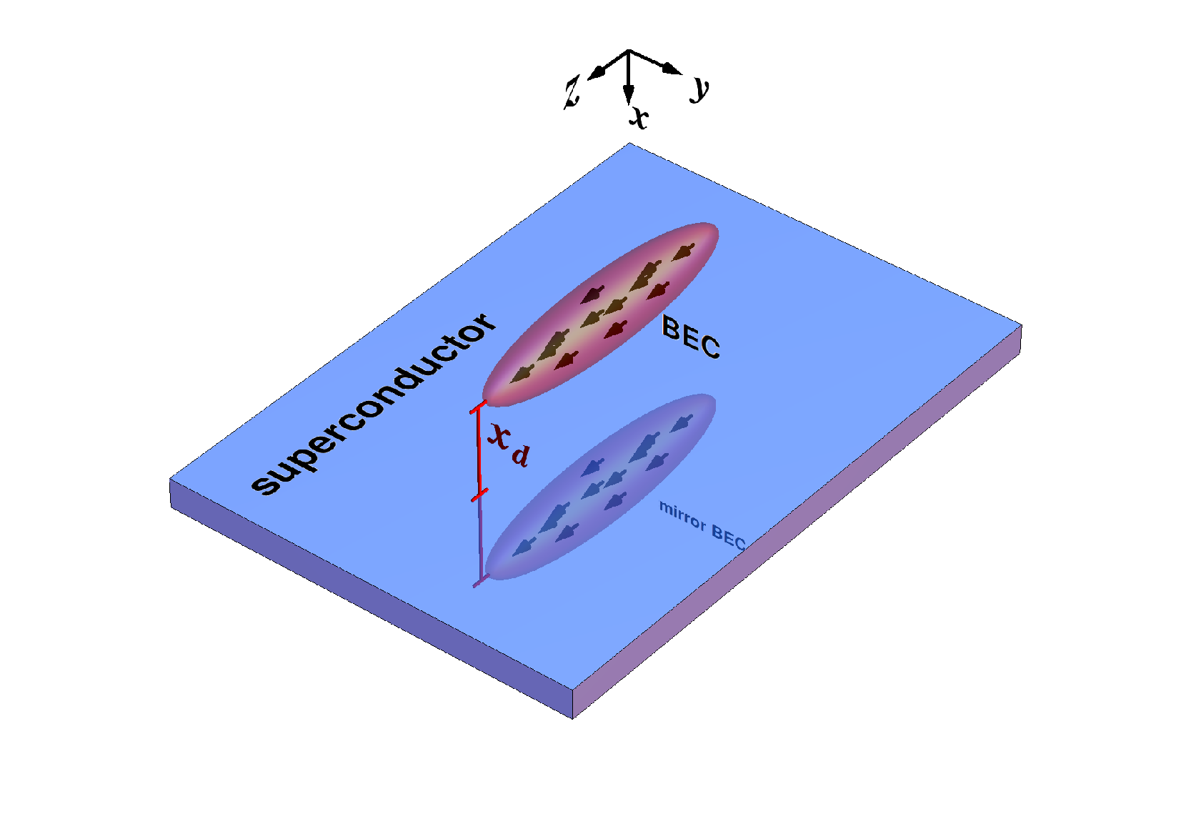
So far, this is the standard way to describe a dipolar BEC. Next we need to include the interaction with the superconducting surface. As described in [34] the magnetic interaction with an infinitely extended superconducting surface can be modeled by the interaction of the BEC with its magnetic mirror, as is depicted in Fig. 1. Every atom in the BEC interacts with every atom in the mirror BEC via magnetic dipole-dipole interaction. We have to add
to the many body Hamiltonian (1). The index denotes the particles in the BEC and the index the mirror particles. Instead of the usual Hartree ansatz (5), we now make the ansatz
| (7) |
It is the Hartree ansatz for a BEC consisting of a mixture of two different kinds of bosons. In our case, is the single body wave function of an atom in the BEC, while describes an atom in the mirror BEC. Theses two kinds of atoms can interact via long ranged dipole-dipole interaction. Also, is not an independent function. It is the shifted mirror function of . Now the task is to minimize
with respect to the single body wave function . This is presented in Appendix A. The resulting GPE reads
| (8) | |||||
II.1.2 Calculation of the mirror term
The mirror term in (8) introduces an additional complication into solving this non-linear Schroedinger equation. Next we want to present an efficient way to calculate this term. First of all we assume that the potential generated by the mirror BEC is small compared to the trapping potential , as well as to the interaction strength between the atoms. If that is the case, then small deviations from the exact shape of will not be significant. As is well known, if the interaction between the atoms becomes large enough, the kinetic term in the GPE can be neglected. This leads to the so-called Thomas-Fermi approximation [38]. Within this approximation the density distribution of a BEC in a harmonic potential takes the guise of an ellipsoid
| (9) |
where , and are the semi-axes of the ellipsoid and is the central density. In the case that there is no dipole-dipole interaction present between the atoms, the semi-axes are given by
| (10) |
In the presence of dipole-dipole interaction the semi-axes are modified [39]. They need to be determined numerically from a set of coupled self-consistency equations [40]. The central density can be determined from the requirement , and is given by .
In the following we will use the Thomas-Fermi approximation to model the mirror BEC. But first let us rewrite . In the case that the external polarizing magnetic field is oriented in the -direction we have and with that
| (11) |
A more convenient way to write this potential is
| (12) |
the first term represents the long ranged part of the interaction and the second term the short ranged part. Since we calculate the interaction between the BEC and its mirror, the delta distribution can never contribute to , so for we get
with
and
| (13) |
With that we have reformulated the task into determining the potential function . Formally, this is the same task as to determine the gravitational potential of an ellipsoidal mass distribution. Chandrasekhar provides a detailed discussion of this type of elliptic integrals in the context of rotating gas clouds [41]. He presents an exact one dimensional representation for , for the case that as well as for . The case is useful if one is interested in calculating the potential between the atoms in the BEC. For example to calculate the semi-axes of a dipolar BEC [40] or its collective modes [40, 42]. Since we want to calculate the potential of the mirror cloud at the position of the actual BEC we need the case . In this case the one-dimensional representation of reads
| (14) |
The function is the ellipsoidal coordinate of the point and is defined by
| (15) |
In the case the lower integration limit of this integral would be . In order to calculate the mirror potential we need the second derivative of with respect to . The detailed calculation can be found in appendix B, here we only present the result
Following Ref. [40] we now introduce the index integrals
| (16) |
and
| (17) |
with . Using the index integrals we can rewrite , which then reads
| (18) |
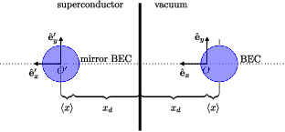
In the numerical calculations the coordinate system is chosen such that the origin coincides with the minimum of the harmonic potential . Expression (18) only holds in , which is the frame of reference where the origin coincides with the center of the mirror BEC. The transformation between the two Systems and is given by , as is depicted in Fig. 2. is the -coordinate of the BEC center-of-mass calculated in . Since the BEC oscillates in the -direction, is a function of time. While is a stationary frame of reference, is co-moving with the mirror BEC opposite to the motion of the BEC. Expressed in the mirror potential takes the guise
| (19) |
Note, that the index integrals, which appear in (18), also depend on the position via the lower integration limit . This means that is not simply a quadratic form. Since the BEC is in motion, is a time dependent quantity, which makes a time dependent potential.
We have now reduced the three dimensional integral in the GPE (8) to four one dimensional index integrals. For a numerical calculation this is already a huge advantage. As it turns out, it is not even necessary to calculate all four integrals, since there exist algebraic relations between the integrals and which can be exploited. This is shown in Appendix D.
II.1.3 Time evolution of the BEC
In order to calculate the time evolution of the BEC we need to solve the time dependent GPE. After all that has been said, the time dependent GPE reads
| (20) |
Here we have introduced the dipole-dipole interaction parameter
| (21) |
It is a dimensionless parameter which measures the strength of the dipole-dipole interaction relative to the strength of the contact interaction. In a harmonic potential the stability of the ground state is only guaranteed if . In the following we will only consider values of that reside in the positive part of this interval. As can be seen from the GPE, the parameter reduces the strength of the contact interaction and introduces a long ranged interaction between the atoms. In order to distinguish the interaction between the atoms in the BEC and the interaction with the superconducting surface, we introduce the parameter . It is defined in the same way as . The only difference is that it describes the interaction with the mirror BEC. While in a real setup those two parameters will always have the same value, we will sometimes choose to be zero, while is non-zero.
Before the time evolution can be calculated, the ground state needs to be determined. To do so, we need to solve the stationary GPE. For this we use a backward Euler method [43, 44, 45, 46], where we calculate the kinetic term using a Fourier transformation. The long ranged part of the dipole-dipole interaction is also calculated with a Fourier transformation. As an external parameter for the numerical calculation we can set the distance between the superconductor and the minimum of the harmonic trap . The actual distance between the BEC and the superconductor slightly differs from this value. The reason for that is the mirror interaction potential, it causes a shift of the minimum of the overall potential. With that, the equilibrium position of the BEC is also shifted. The BEC will not oscillate around the harmonic trap minimum, but around this new potential minimum. However, this shift is so tiny that it can not be detected in an experiment. For this reason we will not discuss it here any further. Once the ground state is determined, we shift the harmonic trap minimum by in the direction to create an initial state for the oscillation of the condensate. After the shift, the distance from the harmonic trap minimum to the surface is . We have now created an excited state, which performs a center-of-mass oscillation around the potential minimum with amplitude . We compute the time evolution with a time-splitting spectral method [43, 45, 46, 47]. Again, the gradient term and the long ranged dipole-dipole interaction potential are taken care of by Fourier transformations. For the spatial discretization of the BEC wave function we use a lattice with periodic boundary conditions. To reduce the computing time, we parallelized parts of the code necessary to calculate a single time step. Those parallel parts of the code were computed on the GPU. We implemented this using CUDA.
In each time step the potential generated by the mirror BEC needs to be determined. The mirror potential is a function of the -coordinate of the center-of-mass position
During a time step the position of the center-of-mass shifts from a position to a position . If we use the position to calculate the mirror potential, we introduce a systematic error into our calculation. To avoid this, we need a method to calculate an effective center-of-mass position for the whole time step, like for example . To calculate we would need the wave function at the end of the time step, which would require a self consistent calculation of every time step. To avoid this, we make use of the time splitting scheme for the time discretization. The Hamiltonian we use in (6) can be separated into two parts , with the kinetic operator and everything else. We then decompose a single time step from to via the Strang splitting method [48], where the time evolution operator is split in three parts. The wave function can be constructed from the wave function using the following scheme:
As can be shown, the application of does not change . So the position of the center-of-mass only changes after has been applied. But since the mirror potential does not contribute to , its shape and strength is not relevant for the first part of the time step. After has been applied, the position of the center-of-mass has shifted to a value . Before we now apply the operator , we calculate the mirror potential using as the effective center-of-mass position for the whole time step. We conclude the time step by applying the operator one more time, which shifts the center-of-mass to its final value .
Besides the -coordinate of the center-of-mass we also keep track of the widths
| (22) |
of the BEC. For a Thomas-Fermi ellipsoid, is connected to the semi-axes via . The analysis of the respective time curves yields information about the excited modes.
II.2 Numerical results for the center-of-mass frequency shift
First we want to study the center-of-mass motion of the BEC. In ref. [34], where we followed the approach of Antezza et al. [36], we have used a simple column density model for the BEC to calculate the frequency shift. This model had the advantage that we were able to get some analytical results for the shift. Now we want to compare the approximate results from the column density model with the results of the numerical simulations. First of all we expect to get good agreement for the case that the oscillation amplitude is small compared to the BEC semi-axis . But even in the case where , we have to expect deviations due to the finite extension of the BEC in the - and -direction, as the column density model is infinitively thin in these directions.
II.2.1 Small amplitude oscillations
In order to improve agreement with the numerical results we can replace the one dimensional column density distribution by a three dimensional Thomas-Fermi density distribution. In the case of small amplitude oscillations, the frequency shift is found to be
| (23) |
where is the center-of-mass oscillation frequency and is the harmonic trap frequency. The function describes the curvature of the potential , which is generated by the mirror BEC
| (24) |
A more detailed derivation of this result is found in Appendix C. The factor of in the function is due to the fact that the mirror BEC moves opposite to the BEC. To account for this we need to take the derivative with respect to rather than to . This leads to a factor of in the second derivative. In order to calculate the function , we again make use of index integrals. The result is a rather long expression, so we will not give it here. The integral which occurs in (23) cannot be further simplified by the use of index integrals, therefore we calculate this three dimensional integral numerically. Here we see the advantage of the column density model, instead of a three dimensional integral, we have a one dimensional integral. The one dimensional integral can be solved analytically, or if one prefers the one dimensional integral can also be solved numerically, which involves just little computational effort.
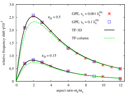
In Fig. 3 we compare the results for the three different models: (a) the numerical simulation, (b) the column density model, and (c) the three dimensional Thomas-Fermi model. The numerical solution of the GPE yields a discrete set of data points for the center-of-mass position at different times . From this we extract the oscillation frequency with the help of a discrete Fourier transformation. For the numerical calculations we use two different oscillation amplitudes, and . Note, that we measure the oscillation amplitude , as well as the distance to the surface , in units of . It is the semi-axis of the Thomas-Fermi density distribution without dipole-dipole interaction, i.e. for . If we used the actual semi-axis instead, the distance and amplitude would depend on . For the results, presented in Fig. 3 and Fig. 4, we used . With that the distance between the BEC and the surface is . Experiments [10, 21], as well as theoretical calculations [25, 26] have shown that such distances are realistic. In Fig. 3 we present the frequency shift as a function of the trap aspect ratio . The other trap aspect ratio remains constant. Here we consider a cylindrical symmetric trap with , which means that . Since the magnetic dipoles are oriented in the -direction, we also have . The central density and the semi-axes shall remain constant for all values of . This is achieved by adjusting the number of atoms in the BEC according to the aspect ratio . If increases, also the number of atoms must increase. The connection between and the number of atoms can be established via the expression for the central density. From this we find . In the numerical calculations for the frequency shift we set the central density to be , where is the central density for the case . The actual central density is somewhat modified due to the dipole-dipole interaction. Fig. 3 shows that in the amplitude range from to the frequency shift does not change. We also find an excellent agreement between the numerical results and the results obtained using the 3D Thomas-Fermi model. Furthermore we can see that the results obtained from the column density model also show a good agreement with the numerical data. The largest deviations can be found for smaller values of , around the position of the maximum frequency shift. For large aspect ratios of the trap the results of all three models converge. If the aspect ratio is large, the BEC is very elongated: . The more elongated the BEC, the better it can be approximated by a one dimensional column density distribution. In the region where the column density model is not a very good approximation. Of course, the accuracy of the column density model also depends on the distance to the surface. However, as we can see the model yields good results for a distance of . For larger distances the accuracy increases. Since smaller distances are likely to be difficult to achieve in experiment, we are not considering them here.
II.2.2 Large amplitude oscillations
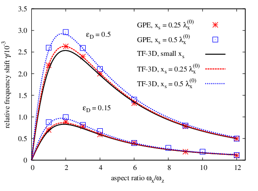
So far we have only discussed small amplitude oscillations and have seen that the resulting frequency shift can be described very accurately using approximation (23). In Fig. 4 we show the results for the frequency shift obtained from numerical calculations with amplitude . Here we clearly see deviations from approximation (23). In order to describe this, we need to consider higher order corrections to the frequency shift. Again, we follow the work of Antezza et al. [36], and the detailed calculation can be found in Appendix C. The resulting expression for the frequency shift reads
| (25) |
with
The results obtained from this approximation are presented in Fig. 4. We calculate the frequency shift for two different oscillation amplitudes, and . As one can see from Fig. 4, the frequency shift increases for larger amplitudes. The results from the numerical calculations show an excellent agreement with approximation (25). For , the correction to the small amplitude case, is only minor. Whereas for , the correction becomes more significant. In the region around the maximum, the correction to the small amplitudes is more important. The more the aspect ratio of the trap is increased, the more do the results for different amplitudes converge.
II.3 Excitation of collective modes due to the BEC-mirror interaction
The center-of-mass motion is not the only collective mode of a BEC where the eddy current effect can be observed. In the following we will focus on the so-called monopole-quadrupole modes [40]. In a harmonic trap the density distribution of a BEC within TF approximation is an ellipsoid. Monopole-quadrupole modes are fluctuations of the density, where the form of the BEC always remains ellipsoidal. This means that the semi-axes become time dependent. Modes of this type can be excited, for example, by a sudden change of the trap frequencies. In a harmonic trap the center-of-mass motion and the monopole-quadrupole modes are decoupled. If the trap minimum is shifted, only the center-of-mass oscillation is excited, while the shape fluctuations remain unaffected. However, if the trapping potential is not purely harmonic, this is no longer the case. The potential generated by the superconducting surface creates an anharmonicity of the potential which leads to a coupling of said modes. If one of the monopole-quadrupole mode frequencies coincides with the center-of-mass oscillation frequency , or with an integer multiple of , a resonant excitation appears. In the vicinity of a resonance the strength of the excitation is enhanced, which increases the chance to observe the effect. In [34] we have discussed this coupling within the framework of an effective anharmonic potential, which included a fourth order term of the form . This term generates a coupling between the center-of-mass motion and the breather mode of the BEC and a resonance occurs when the breather mode frequency matches twice the center-of-mass oscillation frequency. As a measure for the shape fluctuations we observe how the aspect ratio of the BEC changes as a function of time. A discrete Fourier analysis of this data yields information on the strength of the excitation as a function of frequency .
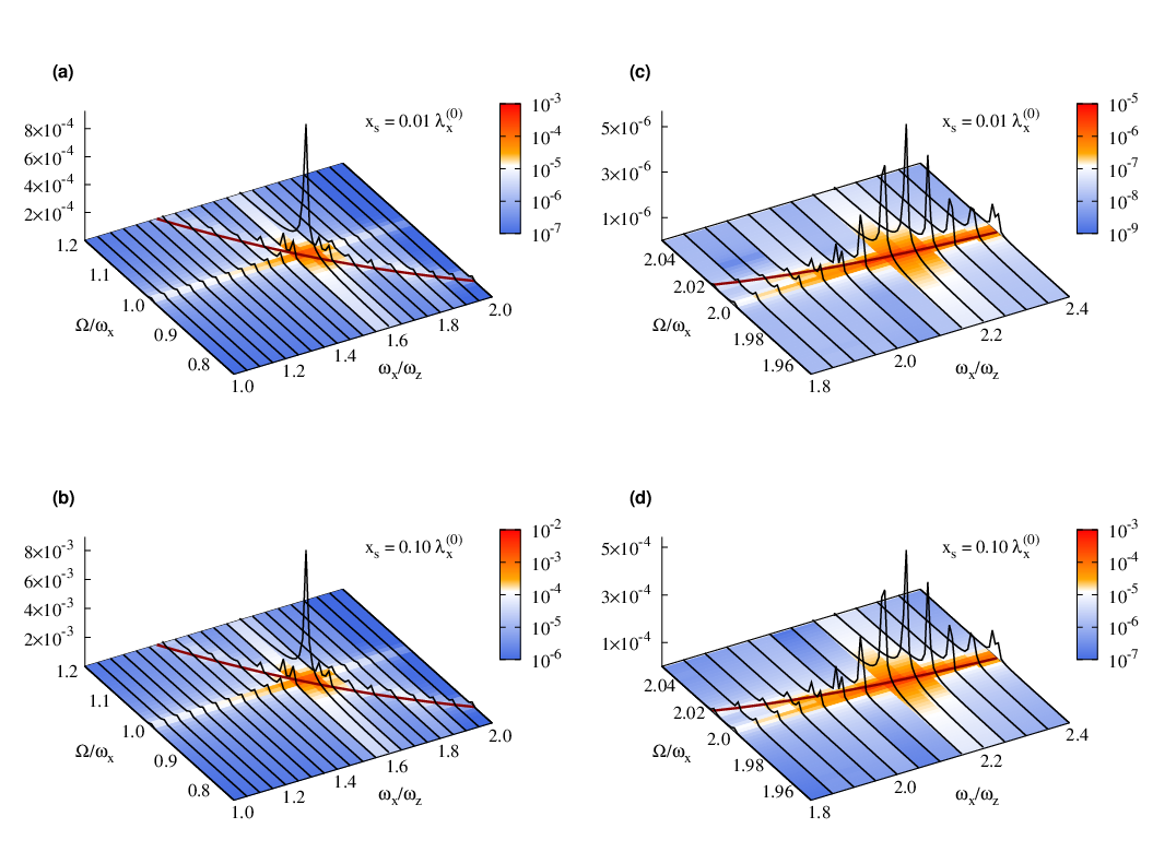
In Fig. 5 we present the frequency spectrum of the BEC aspect ratio , obtained from the numerical solution of GPE (20). We set the dipole-dipole interaction strength to be . We calculated the monopole-quadrupole mode frequencies within the Thomas-Fermi approximation and indicate them in the plots as red lines on the bottom. The simulations were performed for various trap aspect ratios , ranging from to in steps of . The second trap aspect ratio is set to . The spectrum for every aspect ratio is plotted as a black line. The bottom color map shows the excitation on a logarithmic scale, where blue indicates a weak excitation and red a strong excitation. We compare two different oscillation amplitudes, and . We set to be and the central density is . For the -wave scattering length we used the value for chromium, which is [49]. Theses parameters stay the same in every calculation, so that every aspect ratio corresponds to a certain number of atoms in the BEC. One can see that the peaks in the spectra compare quite nicely to the Thomas-Fermi mode frequencies. This means the number of atoms is large enough such that we are within, or at least close to the Thomas-Fermi regime. Fig. 5 (c) and (d) show the section of the spectrum where the breather mode is located. As expected from our previous calculations with the effective potential, we see a resonance at the position where the breather mode frequency and the double oscillation frequency coincide. If we used an symmetric trap with , the breather mode frequency would approach the double oscillation frequency rather than cross it [40]. The strength of the resonance depends of course on the strength of the dipole-dipole interaction parameter and also on the amplitude of the center-of-mass oscillation. In Fig. 5 (c) the oscillation amplitude is and in Fig. 5 (d) it is . While we increase the oscillation amplitude by one order of magnitude, the strength of the resonance increases by two orders of magnitude. This suggests a quadratic dependence of the resonance strength on the oscillation amplitude.
In Fig. 5 (a) and (b) we present a different section of the spectrum. In this section we find the lowest lying monopole-quadrupole mode. Again we find a resonance peak in the spectrum, only this time the resonance occurs at the position where the mode frequency crosses the single oscillation frequency . Again, the oscillation amplitude from Fig. 5 (a) to (b) increases by one order of magnitude. This time, also the strength of the resonance increases by one order of magnitude. From this we can infer that this resonance peak grows linearly with the oscillation amplitude .
To obtain a better understanding of the excitation mechanism, let us simplify the situation as follows. The mirror potential generates an anharmonic perturbation to the harmonic trapping potential. Expanding the mirror potential in a Taylor series yields the involved anharmonic terms. Let us now consider the situation in the rest frame of the center-of-mass. In this frame the anharmonic terms of the potential lead to a time dependent curvature of the potential [50, 51]. For example, if we transform the term into the rest frame, via , the curvature in the -direction gets a time dependent component: . Obviously, this modulates the curvature of the potential in the rest frame with center-of-mass oscillation frequency . A time dependent curvature leads to the excitation of collective modes [52]. If one of the modes happens to have the same frequency as the driving frequency, a resonance occurs. This picture also explains the scaling of the peak height with the oscillation amplitude. The time dependent component which generates the resonance peak at is linear in . In contrast, the term would create a modulation of the form , which drives modes with double oscillation frequency and is quadratic in . This qualitatively explains the scaling of the resonance peak at .
III Frequency shift for a different polarization of the Bose-Einstein condensate
In this section we discuss the dependence of the frequency shift on the orientation of the dipoles. So far we have only considered the case where the dipoles are oriented in the -direction, which is parallel to the superconductor surface and coincides with the long axis of the BEC (see Fig. 1). In principle, the dipoles can be oriented in any direction in which an external polarizing -field can be applied. Since the polarization of the dipoles perpendicular to the surface might be difficult to achieve in an experiment, we will not discuss this case here. However, reorienting the polarization parallel to the surface should not pose a problem. Let us assume that the dipoles are oriented in the -direction, while the direction of the long axis of the BEC remains the -direction. The -direction is still perpendicular to the surface. Compared to the setup we discussed earlier, the dipoles are now rotated by parallel to the surface. The described setup is depicted in Fig. 6 (left panel).
Let us compare the interaction between the dipoles and with the interaction between the dipoles and . The relative orientation between the dipoles remains the same and only the distance changes. This means that only the interaction strength is affected and not the interaction sign. From the center towards the edges of the BEC the interaction strength decreases. Since the interaction sign remains the same, however, all contributions add up constructively to the overall interaction. If we now increase the aspect ratio and add more and more atoms (in such a way that the central density remains the same), then we expect to see an increase of the frequency shift. The frequency shift should increase monotonically with the number of atoms in the BEC.
The situation is different if the dipoles are oriented in the -direction. In this case the interaction sign between and is not the same as between and . Contributions along the -axis of the BEC can cancel each other out. In this case, depending on the length of the BEC, the overall interaction can be smaller than in the case with the dipoles oriented in the -direction. The longer the BEC gets, the smaller is the overall interaction. In the limit the overall interaction, and also the frequency shift, go to zero.
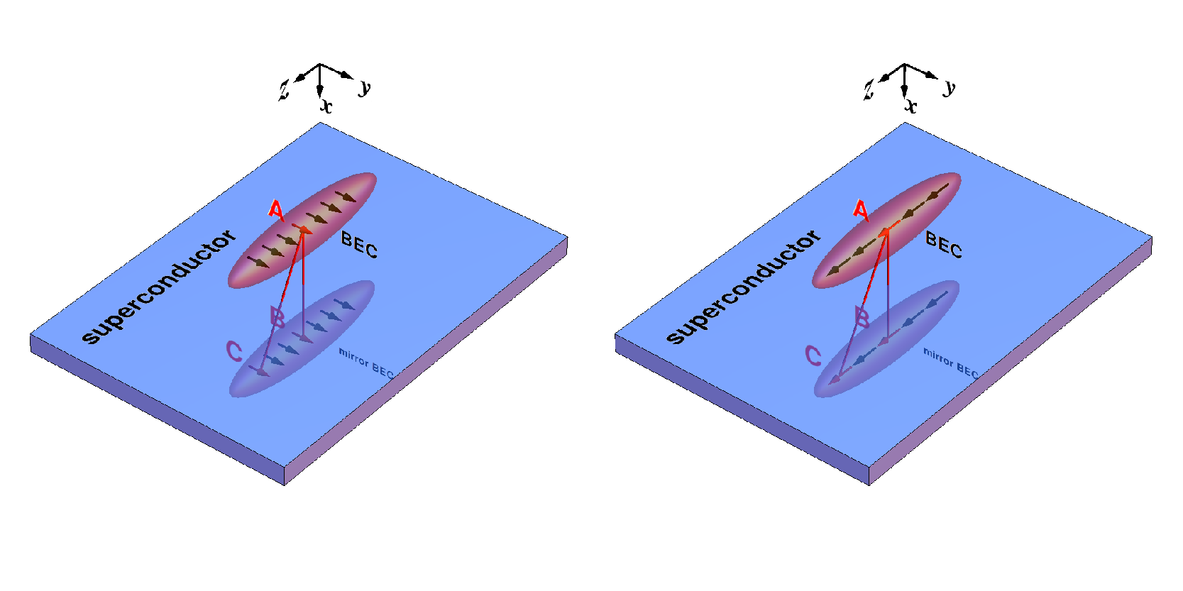
As we have already seen in section II.2, the column density model yields very good results, which is why we will use it here to discuss the configuration with the dipoles oriented in the -direction. The potential along the axes of the BEC generated by the dipoles of the mirror BEC is given by
| (26) |
From this expression we can already see, that the sign of does not change along the axis of the BEC. Given that the semi-axis is known, the expression can be evaluated completely analytically and we obtain the resulting frequency shift with the method already discussed. Here we only give the necessary expressions to calculate the frequency shift, this model is explained in more detail in [34].
| (27) |
with the column density
and curvature change of the mirror interaction potential
The factor in the curvature accounts for the fact that the motion of the BEC leads also to motion of the mirror BEC. In order to calculate the frequency shift one can determine the analytical expressions for (26) and then numerically integrate (27). However, the integral in (27) can also be calculated completely analytical. The result is a very lengthy expression, so we will not give it here but we will present an interesting limit.
We will split the following discussion into two parts. In the first part we will neglect the dipole-dipole interaction between the atoms, meaning we have and . This approach is useful, since it will provide exact analytical results for the frequency shift. In the second part we will include the dipole-dipole interaction, i.e. , and show that resulting corrections are very small.
As we have already mentioned, will increase monotonically as a function of the trap aspect ratio , while the radial semi-axes and the central density are kept constant. For the case , the Thomas-Fermi semi-axes are given by a simple analytical expression (10), and we set . Using the analytical results for and taking the limit we find
| (28) |
This expression only holds for . We will discuss the corrections for below. In [34] we presented a similar value for the case that the dipoles are oriented in the -direction
| (29) |
If we compare the two we see that is roughly by a factor of larger than . By orienting the dipoles in the -direction instead of the -direction the strength of the eddy current effect can be enhanced. The downside is however, that has not the same characteristic shape as , where for an optimal length of the BEC a maximal frequency shift can be observed.
Next, let us see what happens if the dipoles are oriented in an arbitrary direction in the plane parallel to the surface. We will denote the angle between the magnetic dipole moments and the long axis of the Thomas-Fermi ellipsoid with (see Fig. 8). That means we can write the potential generated by the mirror BEC as
The interaction potential is merely a superposition of the two orientations which have already been discussed. This means that also the frequency shift can be constructed from the results we already know. We have
and for the case , we get
| (30) |
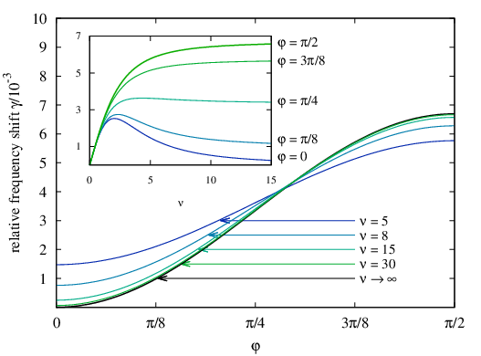
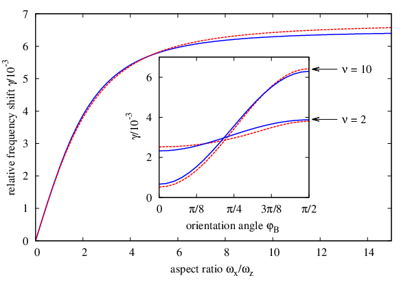
In Fig. 7 we show the frequency shift as a function of the orientation angle . One can see that for the aspect ratio the limit (30) is already a fairly good approximation.
How does the dipole-dipole interaction between the atoms in the BEC itself influence these results? For , there are two effects that need to be considered. Firstly, the dipole-dipole interaction modifies the shape of the BEC. Secondly, the orientation angel between the BEC and the dipoles changes.
The change of the BEC shape has of course also an effect on the frequency shift. For the case that , we get an additional factor in the expression for the frequency shift. In general, this factor needs to be calculated numerically. For the dipoles oriented in the -direction, the expression for the maximal frequency shift reads
If we assume a cylindrical trap with , then magnetic repulsion between the atoms will cause the BEC to become more elongated in the -direction. Thus, we have and the limiting value for is somewhat smaller than given in (28). For a given dipole-dipole interaction strength the factor can be calculated. For we find and for we have . Even for large values of the reduction of is moderate. In Fig. 9 we show for as well as for . There is only a minor difference between the two curves. This shows that expression (28) represents a very good approximation for the maximally possible frequency shift.
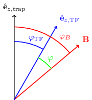
Let us finally discuss the effect of on the orientation angle. Say the external polarizing field is oriented relative to the -axis of the trap in an angle . For the case that , the resulting Thomas-Fermi ellipsoid is neither aligned with the magnetic field nor with the harmonic trap. The resulting configuration is depicted in Fig. 8. This effect is discussed in more detail in Ref. [40]. In order to calculate the frequency shift, we first need to determine the orientation angle of the BEC. This angle depends on , the dipole orientation angle , and also on the geometry of the trap. A set of self consistency equations is given in [40], which can be used to determine the correct angle. Once we have , we can also calculate . In the inset of Fig. 9 we show the frequency shift as a function of for two different trap aspect ratios. It is evident that the influence of is only minor. Comparing the results for to the results for shows that the influence of the dipole-dipole interaction becomes smaller for more elongated traps. In the case of the maximal value for is about , and for its value remains below .
The dependence of the frequency shift on the dipole orientation angle is characteristic for the dipole-dipole interaction between the BEC and its mirror. Therefore it is a fingerprint for the eddy current effect which facilitates its experimental observation.
IV Conclusion
We have studied the effects of the magnetic interaction between a dipolar BEC and a superconductor on the dynamics of the BEC. The dynamical behaviour displays several features that can be used to identify and distinguish this effect from other effects that might play a role close to the surface. In particular we investigate the shift of the center-of-mass oscillation frequency and also the excitation of BEC shape fluctuations.
The first characteristic is the change of the frequency shift with the number of atoms in the BEC. We have discussed this already in Ref. [34], where we used a relatively simple one dimensional model. Here we use more sophisticated models, which show that the previously used model is not exact, but is a very useful tool to obtain analytical results which describes the qualitative behaviour and gives the correct order of magnitude for the effect. Furthermore, we use the improved model to show how the frequency shift increases for large oscillation amplitudes.
Another characteristic is the dependence of the frequency shift on the orientation of the magnetic dipoles of the atoms in the BEC. To investigate this we used the one dimensional model from Ref. [34]. In particular, we discussed the orientations of the dipoles parallel to the superconducting plane. Here, the characteristic dependence of the frequency shift on the orientation angle can be used as a fingerprint of the effect. We also showed that by orienting the dipoles perpendicular to the long axis of the BEC, the effect can be increased by a factor of 2.
To investigate the excitation of collective modes of the BEC, we use the results obtained from the numerical solution of the GPE. The frequency spectrum shows two distinguished resonance peaks. Each peak is connected to certain anharmonic terms in the potential and shows a distinct scaling with the oscillation amplitude. If the trap parameters are chosen properly, these two resonances can significantly enhance the excitation of the collective modes.
In our calculations we assumed a distance of between the superconducting surface and the minimum of the harmonic trap. In Ref. [21] such a distance was demonstrated experimentally in a superconducting microtrap. Theoretical calculations [25, 26] suggest that even shorter distances are possible.
In the experiments thin superconducting strips or wires have been used. In the present work we investigated a superconducting half space. As has been discussed in Ref. [34] a finite superconducting strip needs to meet certain requirements such that this approximation is appropriate. A strip thickness of twice the magnetic penetration depth is sufficient, since the induced eddy currents only flow in the surface area of the superconductor where the magnetic field penetrates the superconductor. The length and width of the strip should be larger than the BEC extensions as well as the distance to the surface. If this is not the case, the effect described here is reduced by a geometrical factor, which depends on the solid angle under which the superconductor is seen by the BEC.
Until now only 87Rb BECs have been combined with superconductors. Due to the small magnetic dipole moments of 87Rb the interaction described here is rather small. However, our results show that the combination of dipolar BECs with superconductors would open up the possibility to study this kind of interaction.
Acknowledgements.
We acknowledge support by the DFG (SFB/TRR 21).Appendix A Derivation of the GPE for a condensate interacting with its mirror
Here we want to show how the GPE for a dipolar BEC close to a superconducting surface can be derived. We will include an interaction term to the many body Hamiltonian and then minimize the energy functional using a Hartree ansatz for the many body wave function. Let us start with the Hamiltonian:
The first part, denoted with , is the standard Hamiltonian. It includes the kinetic term, the external potential, and interaction between the particles in the BEC. The last part of the Hamiltonian, denoted , describes the interaction between the particles in the BEC and the mirror BEC. The index numbers the atoms in the BEC and the index the atoms in the mirror BEC. Since every atom can of course also interact with its mirror, we do not need to make the restriction . Also, every atom interacts with every mirror atom , so that the factor is not needed. Minimizing the functional , under the constraint of particle conservation yields the Gross-Pitaevskii equation (6). Let us now calculate the additional term to this GPE, generated by . We make the following Hartree ansatz
where are the single particle wave functions of the atoms in the BEC and the single particle wave functions of the atoms in the mirror BEC. Of course, a mirror atom does not have an actual wave function. However, this picture is still valid, as long as the wave functions of the atoms and the mirror atoms are well separated. For a better overview we introduce the following abbreviations
Since the operators contained in only act on atoms in the BEC we have
with
>From that we get the usual GPE (6). Additional terms to the GPE arise from . The energy functional reads
For the variational calculation we need to calculate the term . By doing this, we have to keep in mind that and are not independent functions. is the mirror function of , they are connected via
We find
the last line can be obtained by substituting in the second term and using that . >From the minimization of we now find the stationary GPE
Appendix B Calculating the mirror term
Here we calculate the mirror term generated by the mirror BEC. We assume that the density distribution of the mirror has an ellipsoidal shape. We need to determine the second derivative of the potential function given in (14). For the sake of convenience let us define the following function:
with , so that we have
The first derivative with respect to reads
We can say from (15) that , which leads to
With that we find for the second derivative
Let us next determine the derivatives of , the first derivative reads
so that we find
and we therefore get
The second derivative of is given by
so that we obtain our final result
Appendix C Frequency shift of the center-of-mass motion
Here we show in more detail how we derived the results for the frequency shift. We follow the approach of Antezza et al. [36], where they discussed the effect of the Casimir-Polder force on the center-of-mass motion of a BEC. Say we have a BEC in a harmonic trap of the form (4) and the atoms interact with the surface via a potential . The BEC is oscillating in the -direction, which is perpendicular to the surface. Antezza et al. show that in such a case the motion of the center-of-mass is described by the following differential equation
where is the density distribution of the BEC and is the -coordinate of the center-of-mass. For the density distribution of the BEC we use the Thomas-Fermi approximation, which yields the density distribution given in (9). We can now perform the shift and then define the following time dependent function
In the center-of-mass system of the BEC the surface potential appears to be a time dependent potential. Next we expand in terms of . For small amplitude oscillations it is sufficient to linearize . However, if one is interested in corrections due to large amplitudes, the series expansion needs to be performed at least to third order in . The series expansion of can now be inserted back into . We assume that the center-of-mass performs a harmonic oscillation of the form , so that we can expand in a Fourier series . Since we are only interested in the frequency shift, we only need to evaluate the term proportional to . The Fourier coefficient of this term reads
Inserting everything back in the equation of motion for the center-of-mass, the difference between the squares of the frequencies is found to be
In our case the surface potential can be understood as the dipole-dipole interaction potential between the atoms in the BEC and the mirror BEC
where is the density distribution of the mirror BEC. Since we use the Thomas-Fermi approximation, the potential , and its derivatives, are most conveniently calculated using the index integrals. If the dipoles are oriented in the -direction, the potential is essentially given by , for which the expression is presented in (18). As the BEC oscillates perpendicular to the surface, the mirror BEC oscillates as well. However, the mirror BEC oscillates in opposite phase to the BEC. To compensate for this, the above derivatives with respect to need to be replaced by derivatives with respect to :
The reason, that we evaluate the derivatives at the position , is simply the fact that we calculate in the frame of reference where the center of the mirror BEC is at the origin. We will not give the expressions of the derivatives of here, since they are rather long. Finally, we can write , in the case that the difference between the harmonic trap frequency and the frequency of the center-of-mass motion is small. In the case of small amplitudes we can neglect the term quadratic in , which then yields result (23). If we also consider the correction term, we find result (25) for the frequency shift.
Appendix D The index integrals
Integrals of the type
can be calculated numerically using the Carlson method [53]. The algorithm for this is provided in [54]. With that the index integrals
can be calculated via
where the different index integrals have been constructed by a permutation of the arguments of . Actually, we do not need to calculate all three integrals, since there exists a sum rule, which reads
With that it suffices to calculate only two of the three integrals. In the case that the ellipsoid is uni-axial with the solution of these integrals can be given in a closed analytic form:
Again, the sum rule can be used in order to calculate only one of the two integrals. For a spherical BEC with we get
which can be easily seen from the sum rule. In order to calculate the mirror potential we need the index integrals
instead of . By substituting we can obtain from
For the integral the sum rule needs to be modified, it reads
From the single index integrals we now need to construct the double index integrals
with . The two types of integrals are connected via
If we have a uni-axial BEC with , the integral can be solved analytically, it reads
The sum rule for the double index integrals reads
so that we have for example
In the spherical case with the result of the integral reads
With that we have everything at hand to calculate the mirror potential. The index integral and their algebraic properties are also discussed in [40] and [41].
References
- [1] J. Fortagh and C. Zimmermann, Rev. Mod. Phys. 79, 235 (2007).
- [2] M.P.A. Jones, C.J. Vale, D. Sahagun, B.V. Hall, and E.A. Hinds, Phys. Rev. Lett. 91, 080401 (2003).
- [3] P.K. Rekdal, S. Scheel, P.L. Knight, and E.A. Hinds , Phys. Rev. A 70, 013811 (2004).
- [4] T. Nirrengarten, A. Qarry, C. Roux, A. Emmert, G. Nogues, M. Brune, J. M. Raimond, and S. Haroche, Phys. Rev. Lett. 97, 200405 (2006).
- [5] T. Mukai, C. Hufnagel, A. Kasper, T. Meno, A. Tsukada, K. Semba, and F. Shimizu, Phys. Rev. Lett. 98, 260407 (2007).
- [6] D. Cano, B. Kasch, H. Hattermann, R. Kleiner, C. Zimmermann, D. Koelle, and J. Fortágh, Phys. Rev. Lett. 101, 183006 (2008).
- [7] M. Siercke, K. S. Chan, B. Zhang, M. Beian, M. J. Lim, and R. Dumke, Phys. Rev. A 85, 041403(R) (2012).
- [8] B. Zhang, M. Siercke, K. S. Chan, M. Beian, M. J. Lim, and R. Dumke, Phys. Rev. A 85, 013404 (2012).
- [9] H. Imai, K. Inaba, H. Tanji-Suzuki, M. Yamashita, and T. Mukai, Appl. Phys. B 116, 821–829 (2014)
- [10] B. Kasch, H. Hattermann, D. Cano, T. E. Judd, S. Scheel, C. Zimmermann, R. Kleiner, D. Koelle, and J. Fortágh, New J. Phys. 12, 065024 (2010).
- [11] Skagerstam, Bo-Sture K., U. Hohenester, A. Eiguren, and P. K. Rekdal, Phys. Rev. Lett. 97, 070401 (2006).
- [12] U. Hohenester, A. Eiguren, S. Scheel, E. A. Hinds, Phys. Rev. A 76, 033618 (2007).
- [13] R. Fermani, T. Müller, B. Zhang, M. J. Lim, and R. Dumke, J. Phys. B 43, 095002 (2010).
- [14] D. Petrosyan, and M. Fleischhauer, Phys. Rev. Lett. 100, 170501 (2008).
- [15] R. Folman, Quantum Inf. Process. 10, 995–1036 (2011).
- [16] J. Verdu, H. Zoubi, C. Koller, J. Majer, H. Ritsch, and J. Schmiedmayer, Phys. Rev. Lett. 103, 043603 (2009).
- [17] K. R. Patton and U. R. Fischer, Phys. Rev. A 87, 052303 (2013).
- [18] G. Bensky, R. Amsüss, J. Majer, D. Petrosyan, J. Schmiedmayer, G. Kurizki, Quantum Inf. Process. 10, 1037–1060 (2011).
- [19] R. Salem, Y. Japha, J. Chabé, B. Hadad, M. Keil, K. A. Milton, and R. Folman, New J. Phys. 12, 023039 (2010).
- [20] D. Cano, H. Hattermann, B. Kasch, C. Zimmermann, R. Kleiner, D. Koelle and J. Fortágh, Eur. Phys. J. D 63, 17 (2011).
- [21] S. Bernon, H. Hattermann, D. Bothner, M. Knufinke, P. Weiss, F. Jessen, D. Cano, M. Kemmler, R. Kleiner, Do. Koelle, and J. Fortágh, Nat Commun 4, 2380 (2013).
- [22] O. Romero-Isart, C. Navau, A. Sanchez, P. Zoller, and J. I. Cirac, Phys. Rev. Lett. 111, 145304 (2013).
- [23] D. Bothner, M. Knufinke, H. Hattermann, R. Wölbing, B. Ferdinand, P. Weiss, S. Bernon, J. Fortágh, D. Koelle, and R. Kleiner New J. Phys. 15, 093024 (2013).
- [24] D. Cano, B. Kasch, H. Hattermann, D. Koelle, R. Kleiner, C. Zimmermann, and J. Fortágh, Phys. Rev. A 77, 063408 (2008).
- [25] A. Markowsky, A. Zare, V. Graber, and T. Dahm, Phys. Rev. A 86, 023412 (2012).
- [26] V. Dikovsky, V. Sokolovsky, B. Zhang, C. Henkel, and R. Folman, Eur. Phys. J. D 51, 247–259 (2009).
- [27] V. Sokolovsky, L. Prigozhin, and V. Dikovsky, Supercond. Sci. Techn. 23, 065003 (2010).
- [28] T. Lahaye, C. Menotti, L. Santos, M. Lewenstein, and T. Pfau, Rep. Prog. Phys. 72, 126401 (2009).
- [29] A. Griesmaier, J. Werner, S. Hensler, J. Stuhler, and T. Pfau, Phys. Rev. Lett. 94, 160401 (2005).
- [30] K. Aikawa, A. Frisch, M. Mark, S. Baier, A. Rietzler, R. Grimm, and F. Ferlaino, Phys. Rev. Lett. 108, 210401 (2012).
- [31] M. Lu, N. Q. Burdick, S. H. Youn, and B. L. Lev, Phys. Rev. Lett. 107, 190401 (2011).
- [32] A. Frisch, M. Mark, K. Aikawa, F. Ferlaino, J. L. Bohn, C. Makrides, A. Petrov,and S. Kotochigova, Nature 507, 475–479 (2014).
- [33] K. Baumann, N. Q. Burdick, M. Lu, and B. L. Lev, Phys. Rev. A 89, 020701(R) (2014).
- [34] I. Sapina, and T. Dahm, New J. Phys. 15, 073035 (2013).
- [35] D. M. Harber, J. M. Obrecht, J. M. McGuirk, and E. A. Cornell, Phys. Rev. A 72, 033610 (2005).
- [36] M. Antezza, L. P. Pitaevskii, and S. Stringari, Phys. Rev. A 70, 053619 (2004).
- [37] L. Pitaevskii and S. Stringari, "Bose-Einstein Condensation", 2003, Oxford University Press.
- [38] C. J. Pethick and H. Smith, "Bose-Einstein Condensation in Dilute Gases", Second Edition 2008, Cambridge University Press.
- [39] C. Eberlein, S. Giovanazzi, and D. H. J. O’Dell, Phys. Rev. A 71, 033618 (2005).
- [40] I. Sapina, T. Dahm, and N. Schopohl, Phys. Rev. A 82, 053620 (2010).
- [41] S. Chandrasekhar, "Lectures in Theoretical Physics"(University of Colorado Press, Boulder, 1964), Vol. VI, pp. 1-72.
- [42] R. M. W. van Bijnen, N. G. Parker, S. J. J. M. F. Kokkelmans, A. M. Martin, and D. H. J. O’Dell Phys. Rev. A 82, 033612 (2010).
- [43] W. Bao, Y. Cai, and H. Wang, J. Comput. Phys.229, 7874-7892 (2010).
- [44] W. Bao and Q. Du, SIAM J. Sci. Comput. 25, 5 1674-1697 (2004).
- [45] W. Bao, I.-L. Chern, F. Y. Lim, J. Comput. Phys.219, 836-854 (2006).
- [46] W. Bao and Y. Cai, Kinetic and Related Models, 6, 1-135 (2013).
- [47] W. Bao, D. Jaksch, and P. A. Markowich, J. Comput. Phys. 187, 318 (2003).
- [48] G. Strang, SIAM J. Nummer. 5, 505-517 (1968).
- [49] A. Griesmaier, J. Stuhler, T. Koch, M. Fattori, T. Pfau, and S. Giovanazzi, Phys. Rev. Lett. 97, 250402 (2006).
- [50] H. Ott, J. Fortágh, and C. Zimmermann, J. Phys. B 36, 2817 (2003).
- [51] H. Ott, J. Fortágh, S. Kraft, A. Günther, D. Komma, and C. Zimmermann, Phys. Rev. Lett. 91, 040402 (2003).
- [52] F. Dalfovo, C. Minniti, and L. P. Pitaevskii, Phys. Rev. A 56, 4855 (1997).
- [53] B.C. Carlson, Numer. Math. 33, 1 (1979).
- [54] W.H. Press, S.A. Teukolsky, W.T. Vetterling, and B.P. Flannery, "Numerical Recipes in C", Cambridge University Press.