Hubble Frontier Field Free-Form Mass Mapping of the Massive Multiple-Merging Cluster MACSJ0717.5+3745
Abstract
We examine the latest data on the cluster MACSJ0717.5+3745 from the Hubble Frontier Fields campaign. The critically lensed area is the largest known of any lens and very irregular making it a challenge for parametric modelling. Using our Free-Form method we obtain an accurate solution, identify here many new sets of multiple images, doubling the number of constraints and improving the reconstruction of the dark matter distribution. Our reconstructed mass map shows several distinct central substructures with shallow density profiles, clarifying earlier work and defining well the relation between the dark matter distribution and the luminous and X-ray peaks within the critically lensed region. Using our free-form method, we are able to meaningfully subtract the mass contribution from cluster members to the deflection field to trace the smoothly distributed cluster dark matter distribution. We find 4 distinct concentrations, 3 of which are coincident with the luminous matter. The fourth peak has a significant offset from both the closest luminous and X-ray peaks. These findings, together with dynamical data from the motions of galaxies and gas will be important for uncovering the potentially important implications of this extremely massive and intriguing system.
Keywords:
galaxies:clusters:general; galaxies:clusters:MACSJ0717.5+3745 ; dark matter1 Introduction
The standard model of structure formation is built on the conclusion that about 85% of the mass in the universe is of an unknown form which only gravitates. The standard interpretation of this dark matter as massive fermionic particles has, so far, no experimental evidence from sensitive direct searches via nuclear recoil (Akerib et al., 2014) nor have such particles been generated at high energies with the LHC. Astronomically, the most extreme effects of dark matter can be found in massive galaxy clusters, where the general relativistic warp-ing of spacetime leads to extreme lensing distortions on a scale far in excess of that due to the observed stellar or gaseous cluster material. Among all known clusters, MACSJ0717.5+3745 (MACS0717 hereafter, Ebeling et al. (2007)) is one of the most massive and extreme clusters in terms of its mass and temperature, with light deflections of over an arcminute discovered by Zitrin et al. (2009) (Z09 hereafter). This cluster has been exten-sively studied from a multiwavelength perspective providing a unique opportunity to explore the interplay between the visible and dark matter.

Radio observations reveal that this cluster hosts one the most powerful radio halos known to date (van Weeren et al., 2009; Bonafede et al., 2009; Pandey-Pommier et al., 2013). At microwave wavelengths, this cluster is a bright Sunyaev-Zeldovich effect source (Mroczkowski et al., 2012) which has enabled an estimate of its radial velocity through the Doppler shift induced by the plasma in the cluster to the photons of the cosmic microwave background (Sayers et al., 2013). In the optical, a filament of galaxies seems to extend over cosmic scales from the centre of this cluster (Ebeling, Barrett & Donovan, 2004; Medezinski et al., 2013). The same filament can be observed in weak lensing maps (Jauzac et al., 2012; Medezinski et al., 2013) confirming that this cluster represents a ”node” of the cosmic web. Strong gravitational lensing has has uncovered a complex structure where the distribution of lensed images is more anatomical in shape than it is geometrical ( Zitrin etal 2008) so that the strong lensing was not recognised for years despite adequate archival data. Several subclusters may by in the process of simultaneously converging to form one of the largest, complex and most extreme clusters in the universe (Zitrin et al., 2009; Jauzac et al., 2012; Limousin et al., 2012; Mroczkowski et al., 2012). According to Zitrin et al. (2009), this cluster is the largest lens known to date, with an effective Einstein radius of arcseconds. The extreme nature of this clusters is better appreciated in X-rays where the plasma temperature in places may exceed, 20 keV (Ma, Ebeling & Barrett, 2009). The high temperature regions observed in X-rays correlate well with with shocks that are detected in radio maps (Bonafede et al., 2009; Pandey-Pommier et al., 2013). Radio observations have also confirmed that the radio emission is polarized, indicating that the magnetic field is ordered on large scales. The alignment of the radio halo perpendicular to the long axis of the dark matter distribution suggests that the radio emission is the result of a merger-related shock wave, with the emitting particles being shock accelerated (van Weeren et al., 2009). The SZ effect is well mapped in this central region with high resolution Mustang data (Mroczkowski et al., 2012) confirming the pressure enhanced shocked gas and they find a high line of sight velocity for a central gas component of +3600km/s, from a claimed detection of the Kinetic SZE effect, in agreement with the internal galaxy velocity analysis of Ma, Ebeling & Barrett (2009), and nearly orthogonal to the long axis of the dark matter, implying multiple merging.
In this paper we use the recently released data from the Hubble Frontier Fields program11 1 http://www.stsci.edu/hst/campaigns/frontier-fields/ (or HFF hereafter) on this cluster. We use the new data to identify new multiply-imaged systems that are later used to constrain the mass model of this cluster with an unprecedented number of constraints. We use our robust free-form method that does not rely on major assumptions about the distribution of dark matter other than the safe assumption that the galaxy members contain some mass and that more luminous galaxies correspond in general to more massive galaxies.

The paper is organized as follows. We describe the Hubble data in section 2. The lensing data is described in section 3. In section 4 we give a brief description of the reconstruction method. Section 5 presents the results of the lensing analysis. The robusteness of our solution is discussed in more detail in section 6. We discuss our results in section 7, and finally we conclude in section 8.
Throughout the paper we assume a cosmological model with , , . For this model, 1 arcscec equals kpc at the distance of the cluster.
2 HFF data
In this paper we used public imaging data obtained from the ACS (filters: F435W, F606W and F814W) and the WFC3 (F105W, F125W, F140W and F160W), retrieved from the Mikulski Archive for Space Telescope (MAST). The data used in this paper consists of of the data to be collected. Part of the data comes from CLASH (Postman et al., 2012). This release includes the first 40 orbits of observations of MACS0717 from the Frontier Fields program ID 13498 (PI: J. Lotz), also including archival ACS and WFC3/IR data (programs 9722 and 10420, PI.: H. Ebeling; programs 10493 and 10793, PI.: A. Gal-Yam; program 12103, PI.: M. Postman; program 13389, PI.: B.Siana; and program 13459, PI.: T. Treu). Previous observations from earlier shallow imaging (14 orbits in total) are also included in the release , together with the 40 orbits from the HFF campaign. The current release contains 15 orbits in the band F435W, 1 orbit in the band F606W, 30 orbits in the band F814W and 8 orbits in the WFC3 infrared (IR) bands. The relatively low number of orbits in the IR bands makes the current release not ideal for detecting high redshift objects but the deep band at F814W allows us to reliably detect intermediate redshift candidates. In the IR bands we use the background corrected images, corrected for a time-dependent increase in the background sky level (see for instance Koekemoer et al. (2013)). In the optical bands we use the self-calibrated images with improved low-level noise.
From the original files, we produce two sets of color images combining the optical and IR bands. The first set is based on the raw data while in the second set we apply a low-pass filter to reduce the diffuse emission form member galaxies. The second set is particularly useful to match colors in objects that lie behind a luminous member galaxy.

3 Lensing data
Our starting set of strong lensing data is primarily based on the system identification of Zitrin et al. (2009) (Z09). Some systems in Z09 are updated with new spectroscopic redshifts from Limousin et al. (2012); Schmidt et al. (2014) and Vanzella et al. (2014), and also some system definitions are improved following Limousin et al. (2012), Medezinski et al. (2013) and Richard et al. (2014). System 2 was excluded in some previous analyses since this source was too faint. The new and much deeper HFF data confirms this system as a reliable one so we include it in our analysis. Using this set of systems we build a lens-model that is later used to find new candidates taking advantage of the deeper Hubble observations. Many system candidates can be found in the new data set. In this paper, however, we rely only on the most robust sub-sample. This robust sub-sample is defined after we require that the system candidates must have similar colors and morphological features. Also, these systems must be consistent in terms of location in the lens plane and parity with the lens model derived in our first step. In the process of identifying new candidates we need to assume a redshift for the systems. The lower numebr of orbits of the IR bands and the V band (F606W) compared with the F814W band does not allow for precise photometric redshifts of faint objects. Redshifts predicted by the lens models have demonstrated its usefulness and can be competitive with photometric redshifts as shown in Lam et al. (2014). This is particularly true for clusters with shallow mass profiles (like MACS0717) where the shallow mass distribution makes the location of image pairs extraordinarily sensitive to their redshift. We identify 1722 2 At the time of submission of this paper new optical data released through the MAST archive has allowed us to uncover 13 system candidates in addition to the 17 new systems used in this work. These 13 new systems have not been used in this paper but are included in table A2 in the appendix for completeness. Stamps of these new systems are also provided in the website http://www.ifca.unican.es/users/jdiego/MACS0717. new multiple systems that roughly double the original 16 systems in Zitrin et al. (2009); Limousin et al. (2012); Richard et al. (2014). In addition to the new multiple systems we include also 10 elongated arclets (with no identified counter-image) that are helpful to constrain the mass distribution around the critical curves and beyond the Einstein radius. The inclusion of the elongated arclets in our lens model are useful since they incorporate important information about the magnification. This is of particular interest in the regions beyond the Einstein radius where the lensing constraints from multiply lensed images disappear. We include the recently confirmed (spectroscopically) system at z=6.387 as system 19 (following Richard et al. (2014) notation). Our model makes a clear prediction for a third image for this system but it could not be found with the current data. Also, the magnification for the third image is predicted to be significantly smaller () than for the other two images. We should note that in previous works, the original system 19 was considered by other authors as part of our system 18 at z=2.4 but the new system 19 at z=6.387 is completely different (and already used in Richard et al. (2014)). Also, a third counterimage 19.3 is proposed in Richard et al. (2014), very closed to our predicted position. Howevere several faint sources can be seen in that area. The HFF can not confirm nor reject this candidate as it is very faint. Hence we do not use the candidate 19.3 from Richard et al. (2014) in our analysis. More arclets can be identified in the new Hubble images that will be incorporated in future works together with some of the candidates not used in this work and that are expected to be confirmed with the future Hubble data. Our complete strong lensing data set is listed in table A1 in the appendix. Color stamps of the full data set can be found in this website33 3 http://www.ifca.unican.es/users/jdiego/MACS0717. Additional useful material is also included in the same website.

A few examples44 4 Additional examples can be found in this website http://www.ifca.unican.es/users/jdiego/MACS0717 showing re-lensed images involving the previously known system 4 and the new systems 29, 31 and 32 are shown in figure 1. In general, we find a very good agreement between the re-lensed systems and the observed ones. In some cases, differences form the observed arcs highlight deficiencies in our lens model. For instance, the relensed system 32.1’ in figure 1 differs in orientation and magnification from the observed one (32.1). In this case, the spiral galaxy shown in the stamp 32.1 is not included in our lens model that only includes elliptical galaxies. As shown by Diego et al. (2014a), this system could be used effectively to constrain the mass profile of the spiral galaxy, which is acting as a secondary lens.
The relative positions of the images defining our lensing data set is shown in figure 3. Figure 2 shows examples of model predictions for three systems. The grey regions represent the distances (in the source plane but translated into the image plane) between the model prediction and the position of the source (this position is also part of our solution, or array , described below in section 4). The darker the region the more likely a lensed image is to be observed at that position. The positions of the observed arcs are marked with light grey crosses while the position of the observed arcs projected back into the source plane are marked with dark crosses. Based on our model predictions, color information, morpholohy of the galaxies and model-basd parity, we are able to identify all the additional multiple images listed in the appendix. The model predictions are useful to identify possible problesm with teh system identofications like in system 34 in figure 2. The position of the arcs in the source plane do not agree as well as in the other systems higlighting a possible problem with our lens model in this particular region of the cluster or that the redhsift of this system may need to be revised. The new HFF data will help clarify some of these systems and also allow for a firmer identification of other system candidates not used in this work. The model predictions for all the systems can be found in the website55 5 Additional examples can be found in this website http://www.ifca.unican.es/users/jdiego/MACS0717 with the support material. These model predictions show also the expected position of the counterimages that could not be identified wity the current data. Some of these counterimages are predicted to be demagnified versions of the background galaxies buried in the cluster members and hence very unlikely to be uncovered.
Figure 3 shows the full data set together with the critical curve for one of our models (case IV described below in section 4.1).

Although we are confident about our new system identification (they all are consistent with the lens model and show similar colors), it its possible that some corrections are made when the future data arrives (we should remind that we are using 1/3 of the planned data), specially for the unresolved galaxies for which the lack of morphological information does not allow for a more firm confirmation. We should however highlight that since these systems are consistent with the lens model, even in the situation where a few systems are wrongly matched, we don’t expect significant changes in or lens model and/or conclusions in this work.
4 Reconstruction method
We use the improved method, WSLAP+, to perform the mass reconstruction.
The reader can find the details of the method in our previous papers
(Diego et al., 2005a; Diego et al., 2005b; Diego et al., 2007; Ponente & Diego, 2011; Sendra et al., 2014; Lam et al., 2014; Diego et al., 2014b; Diego et al., 2014c).
Here we give a brief summary of the most essential elements.
Given the standard lens equation,
| (1) |
where is the observed position of the source, is the deflection angle, is the surface mass density of the cluster at the position , and is the position of the background source. Both the strong lensing and weak lensing observables can be expressed in terms of derivatives of the lensing potential.
| (2) |
where , , and are the angular diameter distances to the lens, to the source and from the lens to the source, respectively. The unknowns of the lensing problem are in general the surface mass density and the positions of the background sources. As shown in Diego et al. (2005a), the strong lensing problem can be expressed as a system of linear equations that can be represented in a compact form,
| (3) |
where the measured strong lensing observables are contained in the array of dimension , the unknown surface mass density and source positions are in the array of dimension and the matrix is known (for a given grid configuration and fiducial galaxy deflection field) and has dimension . is the number of strong lensing observables (each one contributing with two constraints, , and ), is the number of grid points (or cells) that we use to divide the field of view. In this paper we consider a regular grid of cells covering the field of view shown in figure 3 (4 arcminutes). Each grid point contains a Gaussian function. The width of the Gaussians are chosen in such a way that two neighbouring grid points with the same amplitude produce a horizontal plateau in between the two overlapping Gaussians. is the number of deflection fields (from cluster members) that we consider. In this work we test two different configurations for the deflection field where is equal to 2 (all member galaxies conform a unique deflection field except one foreground galaxy that is placed in a different redshift) or which corresponds to the case where some bright galaxies are treated in an independent way from the rest of the cluster members. Details of these two configurations are given in the next subsection. is the number of background sources (each contributes with two unknowns, , and ). The solution is found after minimising a quadratic function that estimates the solution of the system of equations 3. For this minimisation we use a quadratic algorithm which is optimised for solutions with the constraint that the solution, , must be positive. Since the vector contains the grid masses, the re-normalisation factors for the galaxy deflection field and the background source positions, and all these quantities are always positive (the zero of the source positions is defined in the bottom left corner of the field of view), imposing helps in constraining the space of meaningful solutions. The condition also helps in regularising the solution as it avoids large negative and positive contiguous fluctuations.
4.1 Member galaxy deflections
The member galaxies defining our fiducial galaxy field are all elliptical galaxies selected from the red sequence. The most luminous galaxy in the Hubble image is a known foreground galaxy (2MASX J07173724+3744224) at z=0.1546 (Pandey-Pommier et al., 2013). This galaxy, although well in the foreground ii is still relatively Luminous and hence its mass may have a non-negligible effect in the lens model. Following Zitrin et al. (2009) we include this galaxy in our lens model but set this galaxy to be at z=0.1546. The remaining galaxies in the cluster are assigned a fiducial mass based on their flux. Given the galaxy member positions and masses, , we assume a NFW profile for each galaxy with a scale radius proportional to . A fiducial deflection field is then computed summed from these galaxy members, as their deflections add linearly via the lensing equation. The galaxies are ”split” into different layers to account for possible projection effects and/or some variaiton in the galaxy luminosity-to-mass ratio. Our method re-scales this fiducial field by a constant C per layer and combines it with the fiducial field from a gridded mass distribution to reproduce the observed positions and magnifications of the multiply lensed systems and arclets. For clarity, the layers used in this work are explicitly shown in figure 4 and these additional normalisation parameters are accounted for when calculating the chi-square fit to the data.
The selected galaxies are shown in figure 4. In the same plot we also indicate the galaxies that conform the
different layers. We explore 4 different solutions according to the number of layers used in the reconstruction and/or the number of iterations
in the minimization process.
I) This is the simplest model with two layers for the fiducial field of galaxies.
Layer one contains all the galaxy cluster members at z=0.546 and layer 2 contains the foreground galaxy at z=0.1546.
The solution is obtained after 5000 iterations of the code. This range of iterations was proven in earlier works to be a safe
number to avoid overfitting.
II) as in case I above but we double the number of iterations to 10000. In most cases, at this regime signs of overfitting start to be evident in
the solution like oversized radial critical curves. However, at 10000 iterations these signs are still not present in the solution.
III) as in case I (5000 iterations) but considering 5 layers instead of 2. Like in case I layer 2 contains the foreground galaxy at z=0.1546,
layer 3 contains a big elliptical galaxy at its centre, layer 4 contains another large galaxy south-west of the central galaxy, layer
5 contains 3 large galaxies, 2 above and one below the central galaxy. Finally layer 1 contains all the remaining galaxies.
IV) as in case III but for 10000 iterations.

5 Dark matter distribution
The mass reconstruction is shown in figure 4 for the solution obtained in case IV discussed in the previous section. Together with the mass we show the X-ray emission from Chandra. The Chandra data has been smoothed using the widely used code ASMOOTH, (Ebeling, White & Rangarajan, 2006). The solutions for the other 3 cases are shown in figure 5. The contours in figures 4, and 5 correspond to the smooth component of the mass distribution obtained after subtracting the galaxy contribution to the mass map from the total mass. The first conclusion we can derive from these results is that the mass distribution shows multiple distinct concentrations as shown in Figures 4 and 5. Earlier work has generally claimed 4 peaks in this region (Ma, Ebeling & Barrett, 2009; Limousin et al., 2012; Medezinski et al., 2013). A more precise picture of the location of our peaks can be seen in figure 9 below. Three of our detected maxima correlate well with the observed galaxy and gas enhancements as seen in Figure 9. The third peak on the right side of the image (west) shows a significant offset both with the galaxies and X-rays. Some caution should be exercised with regard to this third peak as we observe have no lensing constraints to help beyond this peak. This subgroup of galaxies does coincide with an X-ray emission peak whereas our mass peak does not , so this is intriguing but certainly would benefit from more clarification. The quality of the Hubble data at the position of this subgroup is significantly poorer than in the rest of the cluster, making it more to identify lensed images in this area but better data to come fem the HFF should help in the near future.
A direct comparison of the 4 solutions discussed in the previous section is shown in figure 6. The agreement between our 4 cases is very clear, indicating that our solution is robust against the assumptions made about the fiducial galaxies or the number of iterations. The same plot shows the comparison with the smoothed X-ray data. In X-rays, several prominent point sources match sources in the HFF data. In figure 6 we label some of them. All the X-ray point sources except one, have a clear counterpart in the HFF field of view. The only exception is source X4 in figure 6. At approximately one arcsecond separation we find a small group of three very faint objects where one of them may be the source of the X-ray emission. Deep follow-up observations at different wavelengths at this position may reveal an interesting object. The source labeled X1 corresponds to the foreground galaxy at z=0.1546. Radio observations reveal that this source either hosts two very powerful radio jets (more likely) or it lies in front of an unusually straight shock front in the cluster (van Weeren et al., 2009) (less likely). In X-rays, the foreground galaxy shows up as a powerful X-ray source, possibly hosting a super-massive black hole at its center, a picture that is in agreement with the observed flattening of the light profile in the centre. This flattening is expected when a super massive black hole is at the centre of a galaxy (Postman et al., 2012; Rusli et al., 2013; Thomas et al., 2014; Lopez-Cruz et al., 2014). Sources X2 and X3 are interesting from the lens model point of view. If we assume that X2 is at redshift z=5, our model predicts that we should expect a counter-image within a few arcseconds of source X3. In the optical, both X2 and X3 share a rather similar morphology with a nucleus surrounded by dusty arms. However in terms of galaxy size, lens magnification and relative orientation, the hypothesis that galaxies X2 and X3 are in fact the same object, loses support. Also, in terms of color galaxy X2 appears significantly redder than galaxy X3.
The profile of the mass model is presented in figure 7. Due to the lack of symmetry of this cluster, the definition, and interpretation of the profile is more challenging than in more relaxed and rounded clusters. In an attempt to capture some of the symmetry of the central DM peak, the centre of the profile in figure 7 is defined at the position of the most massive galaxy that is closest to centre of the most massive peak in our reconstructed mass. This corresponds to group C (see figure 9 below) as defined by Ma, Ebeling & Barrett (2009) (and again in Limousin et al. (2012)). More specifically, the centre is taken at RA=07:17:35.534, DEC=+37:45:0515 (J2000). As found in Ma, Ebeling & Barrett (2009), and later in Limousin et al. (2012), we find that group C is also the most massive. We show the profile of the total mass (dashed) and the grid component after subtraction of the contribution from the galaxies. The profile is strikingly shallow up to a 100 kpc, confirming earlier findings based on parametric methods Zitrin et al. (2009); Limousin et al. (2012); Medezinski et al. (2013). In previous analyses based on data of two other HFF clusters, A2744 and MACS0416, we found also very shallow profiles in the central region (Lam et al., 2014; Diego et al., 2014c) in agreement with results from other authors. The fact that these shallow profiles seem to appear in merging clusters may point in the direction that the shallowness is a consequence of the superposition of smaller halos in the central region. This, however, does not explain why there are not visible cusps associated to the individual halos, and in particular in the dominant halo in group C. Cusps are expected to survive after a cluster merger. In (Diego et al., 2014c) we discuss some additional possible explanations, these include mechanisms related to the baryonic component like feedback or scouring by supermassive black holes that are predicted to flatten the very central part of the galaxies they host. These mechanisms are however unlikely to have a significant impact on scales of tens of kpc. An interesting alternative discussed in the context of another HFF cluster in (Diego et al., 2014c) is the possibility that dark matter has a small, but not negligible, probability of interaction. Simulations have shown that this mechanism, if present, is able to flatten the cusps of cluster halos and on the necessary scales up to 100 kpc (Rocha et al., 2013). In addition to the flattening, if DM interacts, it should exhibit a friction effect that could in principle be studied by possible shifts between the peaks of the DM distribution and the galaxies. To explore in this direction further it is necessary to increase the number of multiple images in the central regions of the cluster in order to constrain better the mass distribution. The future HFF data in this cluster may reveal enough strong lensing information to address the questions arising from our comparison more definitively.

In terms of integrated total mass of our models, we find . However, we should not that our model is largely insensitive to the mass beyond the lensing constraints where our lens model is known to be biased towards lower masses (see Sendra et al. (2014) and references therein) so this mass should be interepreted as the integrated mass within the region defined by the lensing constraints. More meaningful is the total mass associated to the compact galaxy component. We find . In both cases, the errors correspond to the dispersion of the models I,II,III and IV described in the previous section.
6 Variability of the solution
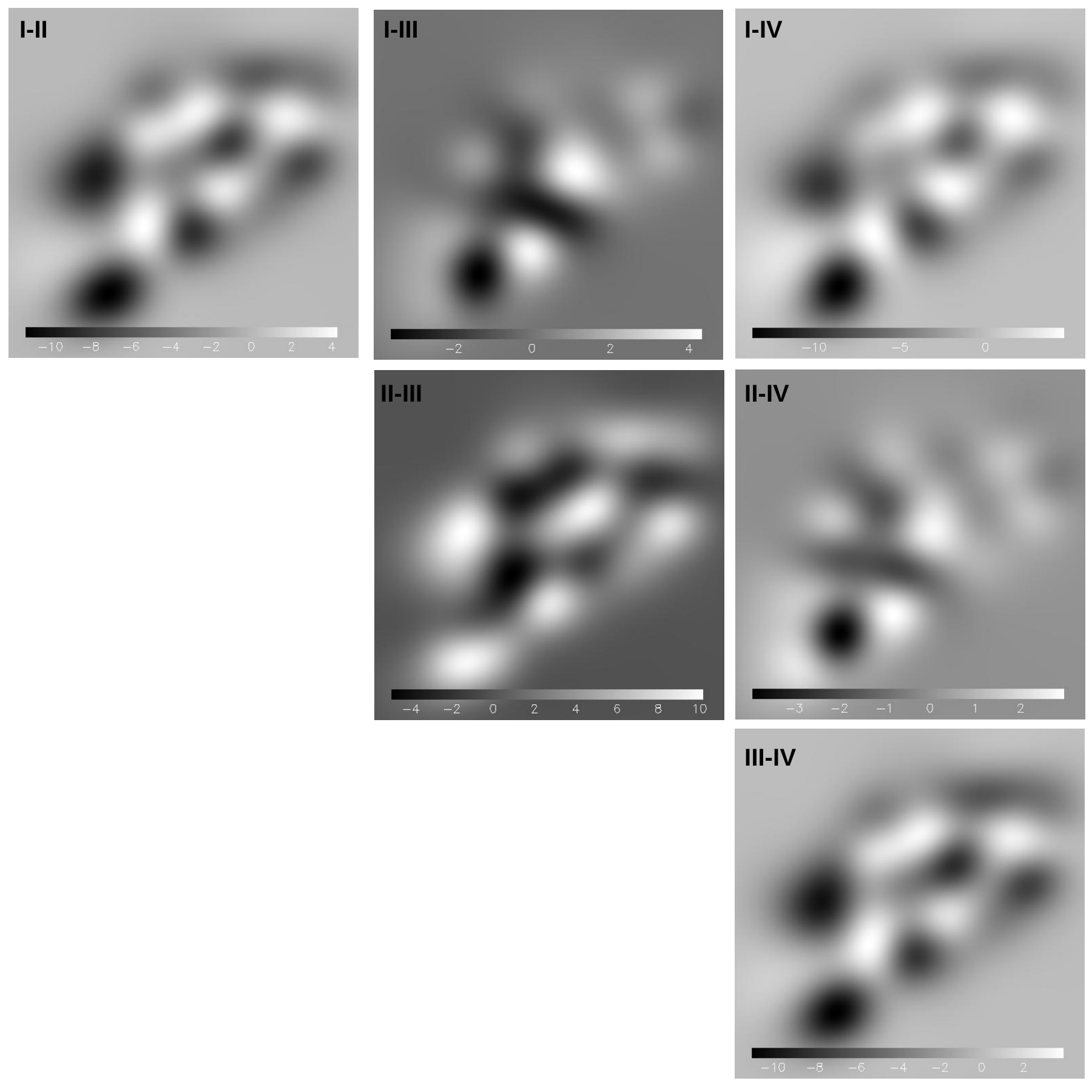
The motivation to produce the different solutions in cases I, II, III and IV is to study the variability of the solution with respect to our input galaxies. As discussed in earlier works, the solution is not unique and an infinite number of models are equally consistent with the data. Typically, the more constraints used in the reconstruction the more similar all these infinite models are. In figure 6, a preliminary comparison of the variability of the solution was presented. The four solutions agree very well in general but also with some small differences that we investigate in more detail in this section. In figure 8 we show the dispersion of the 4 solutions normalized to the mean of the solutions and multiplied by a factor 100 to represent percentages. The largest variation in the solutions occurs in the south-east sector of the cluster. By looking at the individual differences66 6 the individual differences can be found in http://www.ifca.unican.es/users/jdiego/MACS0717 we check that the variability in this part of the lens is larger when comparing cases I-II, and I-III (see figure 10 in the appendix). That is, this variability is mostly due to the increase in the number of iterations. This is not surprising since in this region we find the largest concentration of individual arclets (without counterparts). These constraints, although useful, are weaker than the constraints coming from multiply lensed galaxies. Hence, they become more relevant only at the end of the minimization process. In general, the largest differences concentrate in the region where the lensing constraints disappear.
7 Discussion
The galaxy cluster MACS0717 is one of the most interesting cases for examining the interplay between baryonic and dark matter. Multiwavelength observations of this cluster have revealed powerful radio haloes that trace shock regions. The shocks are probably produced by the near simultaneous merging of several large clusters. This merging geometry can, in principle, be understood better through observations of the kinetic Sunyaev-Zeldovich effect of the gas in the cluster as this is proportional to the velocity along the line of sight (Sayers et al., 2013; Mroczkowski et al., 2012). Analysis of X-ray data confirms the extreme nature of this cluster with temperatures in excess of 20 keV, making this cluster one of the hottest known so far. In terms of mass, this cluster lies in the top end of what is expected for standard models with its mass distribution extending well beyond the field of view covered by the HFF observation. Weak lensing analyses (Jauzac et al., 2012; Medezinski et al., 2013) reveal a filamentary structure towards the south-east from the centre and traced by the elongated galaxy distribution Ebeling, Barrett & Donovan (2004). The point where the filament meets the cluster can be seen in our lens model which shows an elongation iin the south-east part of the cluster and responsible for the highly elongated lensed images we have used in our model.


Previous lensing work has been based on parametric methods (Limousin et al., 2012; Richard et al., 2014), where the central region of the cluster has been divided into 4 separate sub-structures , relying on the optical galaxy distribution. Interestingly the soft component of our mass model, where we have removed the galaxy mass contribution from the total mass also shows a distribution for which 4 density maxima may be reasonably defined (figures 4, 5, and 6. This sub structure is made more evident when we deconvolve partially the smooth component of our mass model. Since the smooth component is a superposition of a grid of Gaussians with a given ”pixel” scale, the resolution of the soft component is limited by the width chosen for the Gaussian. Ideally this grid should be fine enough to follow all relevant substructures, but a partial deconvolution highlights the internal structure of the mass distribution after deconvolution may be even more representative of the true underlying mass distribution. Figure 9 shows the partially deconvolved version of the soft component of the mass distribution for case IV discussed above. When the deconvolved mass distribution is compared with the brightest galaxies from the cluster four components of the mass distribution are now more evident. The correspondence between the location of these galaxy peaks with the general soft mass distribution (after subtracting the member galaxies) is a striking and need not have turned out this way given the freedom of our grid based modelling. In the case of the group A, on the right hand side of the HFF field at the apex of the strongly lensed region, we find a mass peak but we see that its center does not coincide well with the subgroup of what appear to be member galaxies on the upper right corner of the image. As discussed earlier, this could be the result of the lack of lensing constraints beyond that subgroup so certainly the reliability of this peak should not be considered as high as in the other three. Further HFF imaging may help clarify this possible interesting discrepancy. Interestingly, this offset is also found in Limousin et al. (2012) in their blind test analysis (where the mass is not assumed to trace light a priori) highlighting the need for models (like our free-form model) that do not necesarily trace light. Also in Limousin et al. (2012) they also consider a five-component model in their blind analysis that the authors claim does not improve the fit further. However the location of one of their peaks agrees well with the elongation in the south-east part of our model. We should note that according to Ebeling, Barrett & Donovan (2004), and later to Medezinski et al. (2013), a massive filament emerges from this direction of the cluster towards the sout-east, in excellent agreement with our findings (see figure 9). Also it is important to note that Limousin et al. (2012) did not include the arclets in the south-east sector that we used in our analysis, possibly explaining why their fit did not show a significant improvement in their model.
The combined information from radio (shocks), optical, lensing and X-rays emssion it is not clear whether this cluster is in an early phase of merging or it has gone through several core passages already. The radio data shows a region with prominent emission between the B group and the two western peaks (C and D) where X-ray temperatures are also found to be higher. The position and geometry of the radio feature is shown in figure 9 in semitransparent light blue. This picture suggests that group B and groups (C,D) are falling towards each other. On the other hand, measurments of the radial velocity (Ma, Ebeling & Barrett, 2009; Mroczkowski et al., 2012) suggest a significant radial component so combining the radio relic with the velocity measurements it is more likely group B is moving at an angle close to, but not too much, the line of sight. The presence of an extended radio relic in the cluster suggests the system is post first core passage. The foreground galaxy at z=0.1546 lies in the middle of another arc with a straight geometry. This radio emission is likely produced by the AGN at this galaxy and hence not related to the cluster but it could be also a shock front as suggested by van Weeren et al. (2009), although in the same work the authors consider this option as less likely. If this straight feature originates at the cluster instead of the AGN, this could be a fundamental clue to determine the dynamical state of this cluster and would add evidence towards the post-merger hypothesis. In X-rays, the clear offset between the X-ray and luminous (or mass) peaks in group D in figure 9 points to significant dynamical friction from an ongoing merging process. On the other hand, the excellent agreement between the X-ray and mass peaks in group B points to a relatively mild interaction in the past of this group with the cluster environment although a small offset is also expected if B is moving in a path close to the line of sight where projection effects would hide any possible offsets.
Determining the dynamical state of the cluster is important. If the cluster is in the early merging phase, the interpretation that the shallow central profile may be a signature of self-interacting dark matter may be more unrealistic since this mechanism to flatten central cusps are more efficient when clusters collide edge-on (and after first core passage) (Rocha et al., 2013). Of course, this possibility can not be ruled out if this cluster has gone through multiple mergers in the past. A confirmation of the position of the DM peak for group A may lead to important consequences to understand the interplay between baryons and DM.
8 Conclusions
We have derived a free-form solution to the latest HFF data for MACS0717 and in so doing doubled the number of multiple images known. We started by adding those systems initially uncovered by Z09 and later revised and/or measured in Limousin et al. (2012); Medezinski et al. (2013); Schmidt et al. (2014); Richard et al. (2014). We then used this model and the new deeper images from the HFF program to identify 17 new multiply lensed systems doubling the number of known systems. Our method is general so we can make use of pixel positions along the full length of the many faint extended arcs that are visible in the new HFF data. These arcs belong to images comprising multiple systems and also individual long images for which no counter images are expected or which remain unidentified. Using all this information we derive a new lens model. Our new model agrees reasonably well with previous models based on a smaller number of multiply lensed images. We confirm the existence of 4 main concentrations of dark matter in the central part of this cluster. These clumps are still clearly seen even after the contribution from the galaxies is subtracted indicating that the member galaxies must have extended cluster haloes around them. Three of the clumps correlate well with the luminous matter, but less so with the X-ray emission and one of the clumps seem to prefer an area where no significant galaxies (or X-rays) are observed. This, however, could be a systematic effect due to the lack of constraints on this part of the lens. Future data from the HFF program on this cluster will help on improving the lens models even more and will open new opportunities to understand the interplay between baryonic and dark matter in this interesting cluster.
Perhaps the most puzzling result is the very good agreement between some of the peaks of the soft dark matter component and the peaks in the X-ray and luminous matter while other peaks (in particular A and to some degree D) show a significant offset. The highly disturbed nature of this cluster, the offsets observed in some of the groups between X-ray and mass, the elongated critical curve and the presence of prominent radio emission suggest a collision between the groups. An energetic collision between clusters is expected to produce significant offsets between the galaxies (or lensing mass maps) and the plasma, as recently revealed in our HFF analysis of MACS0416 where distinctive offsets indicate this cluster is observed just after first core passage. These offsets are present only in groups A and D. The lack of offsets in group B could be explained by projection effects if B is moving close to the line of sight. The lack of offsets in group C may be understood if C is the most massive group and is less affected by collisions with its larger gravitational field being able to hold on to its gas (X-rays) better that the other groups. The offset between X-ray and mass in group D could be understood if C is moving close to the plane of the sky and towards the centre of mass of the cluster. The offsets in group A are the most difficult to understand although a possible explanation could be the lack of lensing constraints that do not allow to identify the peak at the right position. This is not an unrealistic situation if we realize that strong lensing in this cluster has long been unrecognized in the past despite being the largest gravitational lens known so far (Zitrin et al., 2009).
We also confirm the shallowness of the mass profile. The earlier analysis by Z09 initially found it was very shallow and the largest known lens to date. The shallowness may be due, at least partially, to the accumulated effect of the 4 groups merging into a single massive cluster but could also be an indication of interesting physics related to the properties of dark matter. Detailed simulations of large mergers that incorporate a degree of viscosity in DM may be able to reproduce this degree of shallowness that is known to be present as well in the other HFF clusters analyzed so far Lam et al. (2014); Diego et al. (2014c). New data from the HFF program on this cluster will also help improve the lens models even more, offering new opportunities to understand the interplay between baryonic and dark matter in this interesting cluster.
9 Acknowledgments
This work is based on observations made with the NASA/ESA Hubble Space Telescope and operated by the Association of Universities for Research in Astronomy, Inc. under NASA contract NAS 5-2655. The authors would like to thank the HFF team for making the data for this work available to the community. The scientific results reported in this article are based in part on data obtained from the Chandra Data Archive.77 7 ivo://ADS/Sa.CXO#obs/16305,88 8 ivo://ADS/Sa.CXO#obs/04200,99 9 ivo://ADS/Sa.CXO#obs/01655 We would like to thank Harald Ebeling for making the code ASMOOTH (Ebeling, White & Rangarajan, 2006) available. T.J.B. thanks the University of Hong Kong for generous hospitality. J.M.D acknowledges support of the consolider project CAD2010-00064 and AYA2012-39475-C02-01 funded by the Ministerio de Economia y Competitividad. AZ was provided by NASA through Hubble Fellowship grant #HST-HF2-51334.001-A awarded by STScI. The authors thank Francisco Carrera, Nanda Rea and Marceau Limousin for very useful comments.
References
- Akerib et al. (2014) Akerib D. S. et al., 2014, Physical Review Letters, 112, 091303
- Bonafede et al. (2009) Bonafede A. et al., 2009, A&A, 503, 707
- Diego et al. (2014a) Diego J. M., Broadhurst T., Benitez N., Lim J., Lam D., 2014a, ArXiv e-prints
- Diego et al. (2014b) Diego J. M. et al., 2014b, ArXiv e-prints
- Diego et al. (2014c) Diego J. M., Broadhurst T., Molnar S. M., Lam D., Lim J., 2014c, ArXiv e-prints
- Diego et al. (2005a) Diego J. M., Protopapas P., Sandvik H. B., Tegmark M., 2005a, MNRAS, 360, 477
- Diego et al. (2005b) Diego J. M., Sandvik H. B., Protopapas P., Tegmark M., Benítez N., Broadhurst T., 2005b, MNRAS, 362, 1247
- Diego et al. (2007) Diego J. M., Tegmark M., Protopapas P., Sandvik H. B., 2007, MNRAS, 375, 958
- Ebeling, Barrett & Donovan (2004) Ebeling H., Barrett E., Donovan D., 2004, ApJ, 609, L49
- Ebeling et al. (2007) Ebeling H., Barrett E., Donovan D., Ma C.-J., Edge A. C., van Speybroeck L., 2007, ApJ, 661, L33
- Ebeling, White & Rangarajan (2006) Ebeling H., White D. A., Rangarajan F. V. N., 2006, MNRAS, 368, 65
- Jauzac et al. (2012) Jauzac M. et al., 2012, MNRAS, 426, 3369
- Koekemoer et al. (2013) Koekemoer A. M. et al., 2013, ApJS, 209, 3
- Lam et al. (2014) Lam D., Broadhurst T., Diego J. M., Lim J., Coe D., Ford H. C., Zheng W., 2014, ArXiv e-prints
- Limousin et al. (2012) Limousin M. et al., 2012, A&A, 544, A71
- Lopez-Cruz et al. (2014) Lopez-Cruz O., Anorve C., Birkinshaw M., Worrall D. M., Ibarra-Medel H. J., Torres-Papaqui J. P., Barkhouse W. A., Motta V., 2014, ArXiv e-prints
- Ma, Ebeling & Barrett (2009) Ma C.-J., Ebeling H., Barrett E., 2009, ApJ, 693, L56
- Medezinski et al. (2013) Medezinski E. et al., 2013, ApJ, 777, 43
- Mroczkowski et al. (2012) Mroczkowski T. et al., 2012, ApJ, 761, 47
- Pandey-Pommier et al. (2013) Pandey-Pommier M., Richard J., Combes F., Dwarakanath K. S., Guiderdoni B., Ferrari C., Sirothia S., Narasimha D., 2013, A&A, 557, A117
- Ponente & Diego (2011) Ponente P. P., Diego J. M., 2011, A&A, 535, A119
- Postman et al. (2012) Postman M. et al., 2012, ApJS, 199, 25
- Richard et al. (2014) Richard J. et al., 2014, MNRAS, 444, 268
- Rocha et al. (2013) Rocha M., Peter A. H. G., Bullock J. S., Kaplinghat M., Garrison-Kimmel S., Oñorbe J., Moustakas L. A., 2013, MNRAS, 430, 81
- Rusli et al. (2013) Rusli S. P., Erwin P., Saglia R. P., Thomas J., Fabricius M., Bender R., Nowak N., 2013, AJ, 146, 160
- Sayers et al. (2013) Sayers J. et al., 2013, ApJ, 778, 52
- Schmidt et al. (2014) Schmidt K. B. et al., 2014, ApJ, 782, L36
- Sendra et al. (2014) Sendra I., Diego J. M., Broadhurst T., Lazkoz R., 2014, MNRAS, 437, 2642
- Thomas et al. (2014) Thomas J., Saglia R. P., Bender R., Erwin P., Fabricius M., 2014, ApJ, 782, 39
- van Weeren et al. (2009) van Weeren R. J., Röttgering H. J. A., Brüggen M., Cohen A., 2009, A&A, 505, 991
- Vanzella et al. (2014) Vanzella E. et al., 2014, ApJ, 783, L12
- Zitrin et al. (2009) Zitrin A., Broadhurst T., Rephaeli Y., Sadeh S., 2009, ApJ, 707, L102
Appendix A Compilation of arc positions
| ID | RAJ2000(h:m:s) | DECJ2000(d:m:s) | z | Notes |
| 1.1 | 7:17:34.865 | +37:44:28.39 | 2.963 | S,Z |
| 1.2 | 7:17:34.514 | +37:44:24.43 | 2.963 | S,Z |
| 1.3 | 7:17:33.823 | +37:44:17.88 | 2.963 | S,Z |
| 1.4 | 7:17:32.234 | +37:44:13.13 | 2.963 | S,Z |
| 1.5 | 7:17:37.384 | +37:45:40.95 | 2.963 | S,Z |
| 2.1 | 7:17:34.267 | +37:44:27.72 | 2.500 | |
| 2.2 | 7:17:33.691 | +37:44:21.30 | 2.500 | |
| 3.1 | 7:17:35.645 | +37:44:29.44 | 1.855 | S,Sc |
| 3.2 | 7:17:34.656 | +37:44:21.08 | 1.855 | S,Sc |
| 3.3 | 7:17:37.702 | +37:45:13.86 | 1.855 | S,Sc |
| 4.1 | 7:17:31.440 | +37:45:01.55 | 1.855 | S,Sc |
| 4.2 | 7:17:30.324 | +37:44:40.70 | 1.855 | S,Sc |
| 4.3 | 7:17:33.828 | +37:45:47.77 | 1.855 | S,Sc |
| 5.1 | 7:17:31.169 | +37:44:48.73 | 4.300 | |
| 5.2 | 7:17:30.694 | +37:44:34.19 | 4.300 | |
| 5.3 | 7:17:36.000 | +37:46:02.75 | 4.300 | |
| 5.4 | 7:17:32.657 | +37:44:31.33 | 4.300 | N |
| 6.1 | 7:17:27.434 | +37:45:25.56 | 2.100 | |
| 6.2 | 7:17:27.041 | +37:45:09.90 | 2.100 | |
| 6.3 | 7:17:29.734 | +37:46:11.21 | 2.100 | |
| 7.1 | 7:17:27.970 | +37:45:58.90 | 2.200 | |
| 7.2 | 7:17:27.607 | +37:45:50.87 | 2.200 | |
| 7.3 | 7:17:26.160 | +37:45:06.59 | 2.200 | |
| 8.1 | 7:17:27.982 | +37:46:10.81 | 2.300 | |
| 8.2 | 7:17:26.890 | +37:45:47.41 | 2.300 | |
| 8.3 | 7:17:25.566 | +37:45:06.88 | 2.300 | |
| 12.1 | 7:17:32.438 | +37:45:06.80 | 1.699 | S,Sc |
| 12.2 | 7:17:30.617 | +37:44:34.51 | 1.699 | S,Sc |
| 12.3 | 7:17:33.890 | +37:45:38.38 | 1.699 | S,Sc |
| 13.1 | 7:17:32.522 | +37:45:02.30 | 2.547 | S,Z |
| 13.2 | 7:17:30.610 | +37:44:22.85 | 2.547 | S,Z |
| 13.3 | 7:17:35.083 | +37:45:48.20 | 2.547 | S,Z |
| 14.1 | 7:17:33.305 | +37:45:07.96 | 1.855 | S,Sc |
| 14.2 | 7:17:31.111 | +37:44:22.92 | 1.855 | S,Sc |
| 14.3 | 7:17:35.076 | +37:45:37.19 | 1.855 | S,Sc |
| 15.1 | 7:17:28.253 | +37:46:19.24 | 2.405 | S,Z |
| 15.2 | 7:17:26.090 | +37:45:36.29 | 2.405 | S,Z |
| 15.3 | 7:17:25.584 | +37:45:16.20 | 2.405 | S,Z |
| 16.1 | 7:17:28.589 | +37:46:23.88 | 3.100 | |
| 16.2 | 7:17:26.050 | +37:45:34.49 | 3.100 | |
| 16.3 | 7:17:25.661 | +37:45:13.43 | 3.100 | |
| 17.1 | 7:17:28.646 | +37:46:18.55 | 2.500 | |
| 17.2 | 7:17:26.256 | +37:45:31.82 | 2.500 | |
| 17.3 | 7:17:25.966 | +37:45:12.71 | 2.500 | |
| 17.4 | 7:17:26.592 | +37:45:29.84 | 2.500 | N |
| 18.1 | 7:17:27.406 | +37:46:07.10 | 2.400 | |
| 18.2 | 7:17:26.683 | +37:45:51.66 | 2.400 | |
| 19.1 | 7:17:38.170 | +37:45:16.87 | 6.387 | S,V |
| 19.2 | 7:17:37.860 | +37:44:33.87 | 6.387 | S,V |
| ID | RAJ2000(h:m:s) | DECJ2000(d:m:s) | z | Notes |
| 20.1 | 7:17:29.804 | +37:45:54.42 | 5.000 | N |
| 20.2 | 7:17:29.612 | +37:45:52.62 | 5.000 | N |
| 21.1 | 7:17:28.524 | +37:45:17.94 | 2.000 | N |
| 22.1 | 7:17:28.256 | +37:45:21.23 | 1.500 | N |
| 22.2 | 7:17:28.236 | +37:45:19.91 | 1.500 | N |
| 23.1 | 7:17:31.107 | +37:45:46.47 | 3.000 | N |
| 23.2 | 7:17:30.953 | +37:45:43.14 | 3.000 | N |
| 24.1 | 7:17:28.565 | +37:45:08.76 | 3.000 | N |
| 25.1 | 7:17:31.269 | +37:44:41.10 | 4.500 | N |
| 25.2 | 7:17:31.083 | +37:44:33.92 | 4.500 | N |
| 25.3 | 7:17:36.699 | +37:45:59.07 | 4.500 | N |
| 27.1 | 7:17:35.369 | +37:44:52.50 | 2.000 | N |
| 27.2 | 7:17:35.413 | +37:44:51.16 | 2.000 | N |
| 28.1 | 7:17:37.675 | +37:43:58.70 | 2.000 | N |
| 29.1 | 7:17:36.211 | +37:44:35.43 | 1.800 | N |
| 29.2 | 7:17:34.290 | +37:44:18.97 | 1.800 | N |
| 29.3 | 7:17:37.461 | +37:44:59.83 | 1.800 | N |
| 30.1 | 7:17:34.055 | +37:44:20.78 | 1.800 | N |
| 30.2 | 7:17:37.569 | +37:45:03.96 | 1.800 | N |
| 31.1 | 7:17:29.928 | +37:45:22.68 | 1.750 | N |
| 31.2 | 7:17:29.043 | +37:45:01.98 | 1.750 | N |
| 31.3 | 7:17:31.588 | +37:45:53.94 | 1.750 | N |
| 32.1 | 7:17:28.671 | +37:45:27.87 | 2.700 | N |
| 32.2 | 7:17:31.426 | +37:46:09.57 | 2.700 | N |
| 32.3 | 7:17:27.895 | +37:44:56.93 | 2.700 | N |
| 33.1 | 7:17:32.102 | +37:45:29.53 | 5.000 | N |
| 33.2 | 7:17:32.777 | +37:45:50.83 | 5.000 | N |
| 33.3 | 7:17:28.884 | +37:44:19.29 | 5.000 | N |
| 34.1 | 7:17:33.090 | +37:45:55.36 | 2.300 | N |
| 34.2 | 7:17:30.979 | +37:45:04.33 | 2.300 | N |
| 34.3 | 7:17:29.592 | +37:44:39.16 | 2.300 | N |
| 36.1 | 7:17:27.446 | +37:46:19.25 | 2.500 | N |
| 36.2 | 7:17:25.974 | +37:45:47.89 | 2.500 | N |
| 36.3 | 7:17:24.797 | +37:45:21.06 | 2.500 | N |
| 37.1 | 7:17:35.305 | +37:45:17.08 | 4.000 | N |
| 37.2 | 7:17:35.203 | +37:45:17.08 | 4.000 | N |
| 39.1 | 7:17:36.881 | +37:43:54.51 | 2.000 | N |
| 40.1 | 7:17:40.154 | +37:43:36.19 | 3.000 | N |
| 41.1 | 7:17:37.978 | +37:43:41.06 | 3.000 | N |
| 42.1 | 7:17:39.220 | +37:44:01.71 | 3.000 | N |
| 43.1 | 7:17:34.668 | +37:43:44.25 | 3.000 | N |
| 44.1 | 7:17:36.658 | +37:43:58.23 | 2.000 | N |
| 45.1 | 7:17:33.556 | +37:44:21.12 | 3.000 | N |
| 45.2 | 7:17:32.029 | +37:44:16.37 | 3.000 | N |
| 45.3 | 7:17:37.071 | +37:45:43.00 | 3.000 | N |
| 47.1 | 7:17:38.397 | +37:43:35.46 | 3.000 | N |
| 49.1 | 7:17:36.709 | +37:43:59.64 | 3.000 | N |
| 49.2 | 7:17:34.316 | +37:43:50.64 | 3.000 | N |
| 50.1 | 7:17:29.866 | +37:44:37.45 | 3.000 | N |
| 50.2 | 7:17:31.100 | +37:45:02.55 | 3.000 | N |
| 50.3 | 7:17:34.273 | +37:46:01.85 | 3.000 | N |
| 52.1 | 7:17:28.407 | +37:46:18.27 | 3.000 | N |
| 52.2 | 7:17:26.455 | +37:45:37.79 | 3.000 | N |
| 52.3 | 7:17:25.689 | +37:45:08.95 | 3.000 | N |
| ID | RAJ2000(h:m:s) | DECJ2000(d:m:s) | z |
| 53.1 | 7:17:28.843 | +37:45:40.60 | 2.7 |
| 53.2 | 7:17:31.035 | +37:46:05.71 | 2.7 |
| 53.3 | 7:17:27.619 | +37:44:49.79 | 2.7 |
| 54.1 | 7:17:36.038 | +37:44:42.81 | 1.2 |
| 54.2 | 7:17:35.881 | +37:44:40.50 | 1.2 |
| 55.1 | 7:17:37.391 | +37:43:54.66 | 5.0 |
| 55.2 | 7:17:35.290 | +37:43:44.35 | 5.0 |
| 56.1 | 7:17:34.354 | +37:45:46.06 | 5.0 |
| 56.2 | 7:17:32.964 | +37:45:21.47 | 5.0 |
| 56.3 | 7:17:30.180 | +37:44:08.24 | 5.0 |
| 57.1 | 7:17:34.318 | +37:45:43.93 | 5.0 |
| 57.2 | 7:17:33.131 | +37:45:23.45 | 5.0 |
| 57.3 | 7:17:30.225 | +37:44:06.47 | 5.0 |
| 58.1 | 7:17:34.321 | +37:45:44.60 | 5.0 |
| 58.2 | 7:17:33.078 | +37:45:23.01 | 5.0 |
| 58.3 | 7:17:30.197 | +37:44:06.64 | 5.0 |
| 59.1 | 7:17:34.271 | +37:45:45.49 | 4.0 |
| 59.2 | 7:17:33.116 | +37:45:24.60 | 4.0 |
| 60.1 | 7:17:36.614 | +37:45:48.98 | 2.6 |
| 60.2 | 7:17:31.455 | +37:44:26.40 | 2.6 |
| 60.3 | 7:17:31.351 | +37:44:28.87 | 2.6 |
| 60.4 | 7:17:32.930 | +37:44:28.56 | 2.6 |
| 60.5 | 7:17:31.846 | +37:44:40.95 | 2.6 |
| 61.1 | 7:17:34.125 | +37:45:37.75 | 2.4 |
| 61.2 | 7:17:33.448 | +37:45:26.19 | 2.4 |
| 62.1 | 7:17:31.082 | +37:44:42.36 | 3.0 |
| 62.2 | 7:17:30.965 | +37:44:38.74 | 3.0 |
| 63.1 | 7:17:29.413 | +37:44:58.33 | 3.0 |
| 63.2 | 7:17:29.588 | +37:45:04.63 | 3.0 |
| 64.1 | 7:17:33.044 | +37:44:19.95 | 2.5 |
| 64.2 | 7:17:32.146 | +37:44:18.22 | 2.5 |
| 65.1 | 7:17:33.272 | +37:44:21.32 | 4.0 |
| 65.2 | 7:17:31.682 | +37:44:18.37 | 4.0 |