Alternative links, homogeneous links, and graphs

In [5] Kauffman introduced the class of alternative links and conjectured that the class of alternative links is identical to the class of pseudoalternating links introduced by Murasugi and Mayland in [7]. It was known that all alternative links were pseudoalternating, and it would be shown in [8] that all pseudoalternating links of genus one were alternative, but not necessarily in cases of higher genera, thus resolving Kauffman’s conjecture in the negative. This was done by looking at the intermediary class of homogeneous links which were introduced in [3]. The remaining question is then:

Studying these two classes is interesting because both classes of links have the interesting property of having a minimal genus Seifert surface that can be realized by Seifert’s algorithm ([5],[3]). The difficulty in answering our question lies in the fact that the alternativity of a link is difficult to determine. In this paper we will review homogeneous and alternative links and then give two new characterizations of an alternative diagram. First, in sections 4 and 5 we explain how to construct the enhanced checkerboard graph and the labeled Seifert graph, respectively. In section 6 the definition of a homogeneous link is discussed. The definition of alternative links and our new characterizations of an alternative diagram are discussed in section 7. We conclude with some open questions in section 8. A basic knowledge of knot theory and graph theory is assumed throughout however some preliminary concepts are covered in sections 2 and 3. To avoid confusion, we will refer to a regular projection of an oriented link into the plane as a diagram.

The Seifert Algorithm is a procedure by which one can obtain a surface bounded by a link $L$ from one of its diagrams, [5]. Seifert’s algorithm proceeds as follows. Given a diagram $D$ we smooth all of the crossings according to the following scheme.

Following this procedure produces a collection of oriented circles in the plane bounded by discs. These circles are called Seifert circles. A diagram of $10_{138}$ before and after smoothing the crossings is displayed below.

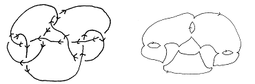
To create a Seifert surface from these circles attach a twisted band to the discs bounding the circles in place of the crossings. The band is twisted in accordance with the smoothed crossing between the two circles. If one circle should be properly contained in another lift the innermost circle from the plane so that it lies above the plane containing the circle that properly contained it. If instead of creating a surface we place the appropriate positive or negative site markers as in [5] we acquire a diagram of Seifert circles with site markers between them instead of crossings. These site markers are shown below.

The components of the complement of the union of Seifert circles are referred to in [5] as spaces. We will refer to the union of circles created by replacing the crossings of a diagram $D$ with site markers as the Seifert diagram, denoted $D_{s}$. Similarly we will denote the collection of spaces in the complement of the union of Seifert circles as $\hat{D}_{s}$. Pictured below is the Seifert diagram of the diagram previously shown.

In this paper we will often refer to the height of a Seifert circle as defined in [6]:

We will also, on occasion refer to the height of a space bounded by a Seifert circle. In this case we are referring to the bounded space in the plane properly contained between Seifert circles or the large unbounded space surrounding the diagram, more formally:

A diagram divides the plane into several regions, including the large outside region surrounding the diagram. We will say that two regions $R_{1}$ and $R_{2}$ of a diagram are touching if they meet at a crossing and we will say that the crossing is incident to both $R_{1}$ and $R_{2}$. For example, the regions $A$, $B$, $C$ and $D$ in the figure below are touching.

Observe that in the above diagram two arcs begin bordering $A$ and stop bordering $D$ at the crossing according to the orientation. Similarly one arc begins bordering $B$ and $C$ and stops bordering $B$ and $C$. We will say that if an arc begins bordering a region $R$ at a crossing $c$ then that arc is going into $R$. Similarly, if an arc ceases to border a region $R$ at a crossing $c$ then the arc is said to be going out of $R$. We then define the following:

In the previous diagram the crossing show is crossing into $A$, out of $D$ and sideswiping $B$ and $C$.

Note that if $R_{1}$ and $R_{2}$ are two regions of a link diagram with a crossing $c$ that is going out of $R_{1}$ and into $R_{2}$ then, upon smoothing the crossings of the diagram according to the Seifert algorithm $R_{1}$ and $R_{2}$ will be joined in the same space of the Seifert diagram. Similarly if there is a crossing out of $R_{2}$ into a region distinct from $R_{1}$, say $R_{3}$, then upon smoothing the crossings $R_{1}$,$R_{2}$, and $R_{3}$ will also all be joined in the same space of the Seifert diagram. We then introduce the following relation:

A basic knowledge of Graph Theory is assumed throughout this paper, however some terms are used frequently enough to merit a restatement of their definitions as taken from [1]:

Pictured below is a graph and it’s smallest nontrivial nonseparable subgraphs:

An example of a graph and it’s blocks is displayed below:

Given a digraph $G$ we denote the in degree of a vertex $v$ as $\delta^{-}(v)$, the outdegree of $v$ as $\delta^{+}(v)$ and the degree of $v$ as $d(v)=\delta^{-}(v)+\delta^{+}(v)$. We will also the use the following theorem from section 2.4 of [1]:

Let $D$ be a diagram. Checkerboard color the diagram as in [5]. We can construct a signed planar digraph $\Phi(D)$ called the enhanced checkerboard graph from this diagram in the following way. Assign a black vertex to each black region and a white vertex to each white region including the large “outside” region of the diagram. Two vertices are connected by a directed edge labeled either $+$ or $-$ according to the scheme shown below. A clarification of how loops are handled is also shown.

To more clearly illustrate how $\Phi(D)$ is constructed a colored diagram and the corresponding $\Phi(D)$ of $10_{138}$ are shown below. Note that, by construction $\Phi(D)$ is necessarily planar. This is due to the fact that our diagrams come from regular projections which only admit single and double points.

A similar graph construction is explained in [6] from which we borrow the $\Phi$ notation.

In other words, $\Phi(D)$ is an even graph and has a cycle decomposition that is to say every edge is a part of a cycle.

We can then view a component of $\Phi(D)$ as a characterization of the site markers in a particular space of a given $\hat{D}_{s}$.

As shown in [3] we can construct the Seifert graph of a diagram from it’s corresponding Seifert diagram. This is done by assigning a vertex to each Seifert circle and a signed edge labeled either $+$ or $-$ between two vertices for every site marker between their corresponding Seifert circles. The sign of these edges is determined by the marker it corresponds to. Edges with the same label correspond to markers of the same type. More precisely, a negative site marker corresponds to a negatively signed edge and positive site markers a positively signed edge. For clarity we will represent positive edges as solid and negative edges as hashed. We will say that two edges are of the same type if they are both solid or are both hashed. An example of a Seifert graph from the same diagram of $10_{138}$ that we have used in previous sections is displayed below.

Here we define an extension of the Seifert graph that we call the labeled Seifert graph defined in the following way,

When we consider a labeled Seifert graph constructed from a particular diagram $D$ we denote that graph as $G(D)$. $G(D)$ is constructed in the same way as the original Seifert graph with the only addition being that the vertices are labeled with the height of the Seifert circle that they correspond to. This is to say if $C$ is a Seifert circle with $h(C)=i$ then the corresponding vertex in $G(D)$ is labeled with an $i$. Displayed below is the same Seifert graph as before only now as a labeled Seifert graph:

Consider an arbitrary labeled Seifert graph $G$. Let $G_{i}$ be the subgraph of $G$ constructed in the following way. Delete all vertices $v$ such that $h(v)<i-1$ or $h(v)>i$. Then delete all edges between vertices of height $i-1$. This potentially disconnected subgraph is $G_{i}$. We will refer to all $G_{i}$’s as height subgraphs. Observe that $G=\bigcup_{i=0}^{n}G_{i}$ where $n$ is the maximum height of a circle in the Seifert diagram. For clarity, when discussing a labeled Seifert graph constructed from a diagram $D$ we will denote the height subgraphs as $G_{i}(D)$. For example, in the figure below are the $G_{i}(D)$’s for the same projection of $10_{138}$ we have been using.

Homogeneous Links were defined in [3] in the following way.

Note the following result from [6]:

Given that our labelled Seifert graph is an extension of the Seifert graph this result will hold for labelled Seifert graphs as well. From this we may conclude the following:

Recall that in the construction of the Seifert diagram crossings are replaced with positive or negative site markers. Two markers are said to be of the same type if they are both positive or are both negative. A space in the Seifert diagram may contain one, two or zero marker types. We then have the following definition from [5]:

We can recharacterize this definition in the context of the spatial graph of a diagram, but first we will need the following definition.

We can also recharacterize the definition of an alternative diagram in terms of the labeled Seifert graph.

We may then present our main theorem, a recharacterization of an alternative diagram in the context of labeled Seifert graphs.

It was noted in [3] that all alternative link diagrams are homogeneous. This is easy to see because if a labeled Seifert graph is alternative then all of its $G_{i}(D)$’s are alternative which would imply that the blocks contained in each $G_{i}(D)$ are homogeneous. However, not all homogeneous diagrams are alternative. Below are two diagrams of a $9_{43}$ with their respective labeled Seifert graphs. The second diagram is alternative and homogeneous while the first diagram is homogeneous, but not alternative.

Similarly, it is not the case that all minimal crossing diagrams of a homogeneous link are homogeneous as can be seen in the infamous “Perko Pair” which answers question 1 from [3]. This example also shows that minimal crossing diagrams of alternative links are not necessarily alternative. Note that $10_{161}$ might not the smallest homogeneous link that has a nonhomogeneous minimal crossing diagram. All minimal crossing diagrams of alternating links are alternating and therefore homogeneous and alternating. It must then be that such a minimal example is nonalternating. The smallest nonalternating homogeneous link is $8_{19}$, [3]. The sequence of Reidemeister moves between the two diagrams of $10_{161}$ with the corresponding spatial and labeled Seifert graphs are included in the appendix.

In [3] the question was asked as to whether or not every homogeneous link has a homogeneous minimal crossing diagram. It is then natural to ask the same of alternative links.

There is a complete classification of homogeneous knots up to 9 crossings in [3]. All homogeneous links up to $10_{134}$ can be seen to be alternative from their minimal crossing diagrams given on [2]. The first homogeneous knot listed that is not immediately identifiable as alternative is $10_{138}$.

Presented here is the Reidemeister sequence between the two diagrams of the Perko Pair. At each step the knot diagram is on the left and the corresponding spatial and labeled Seifert graph are on the center and right respectively.

References

- [1] J.A. Bondy, U.S.R. Murty, Graph Theory, Springer, 2008.
- [2] J. C. Cha and C. Livingston, KnotInfo: Table of Knot Invariants, http://www.indiana.edu/ knotinfo, (May 13, 2014).
- [3] P. Cromwell, Homogeneous Links, J. London Math. Soc. (2), 39 (1989), 535-552.
- [4] S. Hugget, I. Moffattt, N. Virdee, On the Seifert Graphs of a link diagram and its parallels, Math. Proc. Cambridge Philos. Soc., 153 (2012) 123-145.
- [5] L. Kauffman, Formal Knot Theory, Dover Publications, (2006).
- [6] P. Manchn, Homogeneous links and the Seifert matrix, Pacific Journal of Mathematics, (2), 255 (2012) 373-392.
- [7] E.J. Mayland, K. Murasugi, On a structural property of the groups of alternating links, Can. J. Math., (3), 28 (1976), 568-588.
- [8] M. Silvero, On a Conjecture by Kauffman on Alternative and Pseudoalternating Links, arXiv:1402.4599 [math.GT].