Gauge invariant surface holonomy and monopoles
Abstract.
There are few known computable examples of non-abelian surface holonomy. In this paper, we give several examples whose structure 2-groups are covering 2-groups and show that the surface holonomies can be computed via a simple formula in terms of paths of 1-dimensional holonomies inspired by earlier work of Chan Hong-Mo and Tsou Sheung Tsun on magnetic monopoles. As a consequence of our work and that of Schreiber and Waldorf, this formula gives a rigorous meaning to non-abelian magnetic flux for magnetic monopoles. In the process, we discuss gauge covariance of surface holonomies for spheres for any 2-group, therefore generalizing the notion of the reduced group introduced by Schreiber and Waldorf. Using these ideas, we also prove that magnetic monopoles form an abelian group.
Key words and phrases:
Surface holonomy, gauge theory, 2-groups, crossed modules, higher-dimensional algebra, monopoles, gauge-invariance, non-abelian 2-bundles, iterated integrals1. Introduction
1.1. Background, motivation, and overview
Ordinary holonomy along paths for principal group bundles has been studied for over 40 years in the context of gauge theories in physics and in the context of fiber bundles in mathematics. Recently, with ideas from higher category theory, it has been possible to extend these ideas to holonomy along surfaces. Although higher holonomy, and more generally higher gauge theory, has been studied in the context of abelian gauge theory for higher-dimensional manifolds, it was thought for some time that non-abelian generalizations were not possible [Te86]. Today, we understand this as being due to the fact that a group object in the category of groups is an abelian group. By “categorifying” well-known concepts, and considering group objects in the category of categories, one can avoid this restriction. The language of higher categories allows us to give a resolution to this problem.
The data needed for defining surface holonomy for abelian structure groups has been known for quite some time under the name abelian gerbes with connection with a formal presentation offered by Gawedzki [Ga88] in 1988 in the context of the WZW model, with further work in 2002 with Reis [GaRe02]. Further development under the name of non-abelian gerbes, higher bundles, and so on were carried out in the following years starting with the foundational work of Breen and Messing [BrMe05] in 2001, where the data for connections on non-abelian gerbes first appeared. In [BaSc04], Baez and Schreiber gave a definition of non-abelian gerbes with connection in terms of parallel transport using the notion of a 2-group. The most up-to-date theoretical framework in terms of category theory, which provides a language easily adaptable for non-abelian generalizations, was established by Schreiber and Waldorf in [ScWa13]. In this categorical setting, higher principal bundles with connections are described by transport functors.
The motivation for transport functors comes from observations originally made by Barrett in [Ba91] and expanded on by Caetano and Picken in [CaPi94] by describing a bundle with connection in terms of its holonomies. In [ScWa09], Schreiber and Waldorf use a categorical perspective to prove that a principal group bundle with connection over a smooth manifold determines, and is determined by, a transport functor defined on the thin path groupoid of that manifold with values in a fattened version of the structure group viewed as a one-object category. The upshot of this equivalence is that it is conceptually simple to go from categories and functors to 2-categories and 2-functors. In [ScWa11], [ScWa], and [ScWa13], Schreiber and Waldorf take advantage of this equivalence and abstract the definition so that it can be used to define principal 2-group 2-bundles with connection allowing a conceptually simple formulation of surface holonomy.
In the present article, we review the theory of transport functors formalized by Schreiber and Waldorf in [ScWa09], [ScWa11], [ScWa], and [ScWa13] with an emphasis on examples and explicit computations. Besides this, we accomplish several new results. First, we provide a definition of holonomy along spheres modulo thin homotopy without representing a sphere as a bigon (Definition 3.42). The target of this holonomy is an analogue of conjugacy classes, which is used for ordinary holonomy along loops, called -conjugacy classes. To prove this, we introduce a procedure that turns an arbitrary transport functor into a group-valued transport functor. In [ScWa13], the authors forced their surface holonomy to land in a rather restrictive quotient of the structure 2-group to prove gauge invariance of holonomy. Our perspective is to take the smallest quotient possible, and we show our quotient surjects onto the one of [ScWa13].
We then focus on transport functors with a particular class of 2-groups, termed covering 2-groups, given by a Lie group and a covering space of We provide a simple formula, motivated by constructions in [HoTs93], for holonomy along surfaces in a local trivialization and show that this formula agrees with the surface-ordered integral in [ScWa11]. This gives an interesting relationship between (i) well-known formulas in the physics literature for computing the magnetic flux in terms of a loop of holonomies and (ii) non-abelian surface-ordered integrals in terms of 1- and 2-forms of [ScWa11]. Physically, we argue that the latter is the correct analogue to computing the magnetic flux as a surface integral and our formula tells us that this agrees with the usual definition given in the physics literature. This is all done without the introduction of a Higgs field, completing the ideas in [GoNuOl77].
Then we consider an entire collection of examples of transport 2-functors constructed from an ordinary principal -bundle with connection along with a choice of a subgroup of the fundamental group of (such a choice of subgroup determines a covering 2-group). We show that when the subgroup is chosen to be itself, our example reduces to the curvature 2-functor defined by Schreiber and Waldorf in [ScWa13]. We instead focus on the other extreme, namely when the subgroup is chosen to be the trivial group to calculate four examples of surface holonomies associated to both abelian and non-abelian magnetic monopoles. But just as ordinary holonomy is not exactly group-valued on the space of all loops (due to conjugation issues), surface holonomy isn’t in general either. Using our results on gauge invariance of sphere holonomy for arbitrary 2-groups, we prove that the surface holonomies for magnetic monopoles are not only gauge invariant but also form an abelian group.
1.2. Outline of paper along with main results
In Section 2, we review the main definitions of transport functors along with an equivalence between local descent data and global transport functors. We follow the recent work of Schreiber and Waldorf [ScWa09] who describe it precisely and categorically in a framework that is suitable for generalizations to surfaces. We briefly discuss the relationship to principal -bundles with connection, where is a Lie group, in their usual formulation by introducing the category of -torsors (manifolds with free and transitive right -actions). The equivalence between the two descriptions was proved in [ScWa09]. We also review the relationship between local descent data and differential cocycle data for principal group bundles, recalling the well-known formula for parallel transport in terms of a path-ordered integral. To obtain group-valued holonomies, we introduce a procedure (60) described as a functor that takes an arbitrary transport functor and produces a group-valued transport functor in Section 2.8. The presentation differs a bit from that of [ScWa09] so we describe it in some detail.
In Section 3, we review how to ‘categorify’ the definitions and statements of Section 2 in order to define transport 2-functors. The main references for this section include [ScWa11], [ScWa], and [ScWa13]. We only briefly review the technical points but spend more time on a computational understanding of surface holonomy and also supply an iterated integral expression for surface holonomy including a picture (Figure 15) that we think will be useful for lattice gauge theory. As in the case of holonomy along loops, we introduce a procedure (169) to obtain group-valued surface holonomy. This lets us discuss gauge covariance and gauge invariance simply and in full detail without referring to the reduced group of [ScWa13]. However, we restrict ourselves to holonomy along spheres as opposed to surfaces of arbitrary genus. We show, in Theorem 3.41, that our holonomy along spheres lands in a set that surjects onto the reduced group and give a simple example, in Lemma 3.46, where this surjection has nontrivial kernel.
In Section 4, we consider transport 2-functors with structure 2-group given by a covering 2-group. We give a new and simple formula valid for all such transport 2-functors in Corollary 4.19 for surface holonomy in a local trivialization in terms of homotopy classes of paths of holonomies along loops. This construction was inspired by work of physicists for computing magnetic charge as a topological number [HoTs93]. In Definition 4.14, we give our main construction of a transport 2-functor, called the path-curvature 2-functor, associated to every principal -bundle with connection and to any subgroup of We prove that this assignment is functorial. Furthermore, the path-curvature 2-functor is shown to reduce to the example of Schreiber and Waldorf known as the curvature 2-functor in [ScWa13] when the subgroup of is chosen to be itself. We describe this construction on four levels: (i) global transport functors (ii) functors with smooth trivialization data chosen (iii) descent data (iv) differential cocycle data. This allows one to work with either construction at whatever level he or she pleases. We then summarize our result as a list of commutative diagrams of functors in (251), (255), and (257).
In Section 5, we consider special cases of covering 2-groups and give several examples all of which are known as magnetic monopoles [HoTs93]. The first example is obtained from any principal -bundle with connection over the two-sphere It is shown that the surface holonomy along this sphere coming from the path-curvature 2-functor defined in Section 4 is precisely the integral of the curvature form of the principal -bundle along this sphere, which in this case is the integral of the first Chern class over the sphere. This example is precisely the Dirac monopole [Di31] and the surface holonomy gives the magnetic charge as the integral of a magnetic flux. We then discuss non-abelian examples starting with a principal -bundle with connection over the sphere and compute the surface holonomy explicitly using both our simple formula and the formula in terms of path-ordered integrals using differential forms. In the case of a non-trivial bundle, the surface holonomy along the sphere is given by the element in the universal cover of which is the nontrivial element in the kernel of the covering map We do this same computation in other examples including where is the center of and also for the case This gives a rigorous meaning to the notion of non-abelian magnetic flux as a surface holonomy along a sphere (see Definition 5.1). Furthermore, it is shown that magnetic flux is a gauge-invariant quantity in Corollary 5.2.
Finally, the Appendix includes an overview of diffeological spaces which are used to describe several of the constructions involving infinite-dimensional manifolds and smooth maps between them.
In short, this article contains the following results.
- •
- •
Theorem 3.41 accomplishes the analogous result for surface holonomy along spheres in Definition 3.42. The image lands in -conjugacy classes (Definition 3.40) instead of the reduced group of [ScWa13]. The set of -conjugacy classes surjects to the reduced group but is not in general injective as shown in Lemma 3.46. We also prove that the fixed points of this action form a central subgroup of the group of surface holonomies in Lemma 3.48.
- •
The rest of the paper focuses on transport 2-functors whose structure 2-groups are covering 2-groups (Definition 4.7). They are called path-curvature 2-functors (Definition 4.14). These transport 2-functors are defined without using surface integrals, and we show, in Theorem 4.18 and Corollary 4.19, that locally, any transport 2-functor (defined as in [ScWa11] using surface integrals) with structure 2-group a covering 2-group, coincides with ours, thus enabling a simple formula for calculating surface holonomy.
- •
Section 5 includes several examples and explicit computations of surface holonomy. Due to the previously mentioned theorem, these examples can rightfully be called magnetic fluxes of magnetic monopoles from physics. We include several examples of non-abelian surface holonomy. We conclude with Corollary 5.2 that shows that the magnetic flux is a fixed point under the action and therefore lands in the central subgroup mentioned earlier. In particular, this implies that the magnetic charge is an abelian group-valued quantity known as a topological number.
1.3. Acknowledgments
Firstly, we thank Scott O. Wilson who helped greatly during the entire process of this work, providing ideas and proofreading drafts. Secondly, we thank V. Parameswaran Nair who made suggestions related to this work and informed us of references including [GoNuOl77]. We have benefited from conversations with Gregory Ginot, Jouko Mickelsson, Urs Schreiber, Stefan Stolz, Rafal Suszek, Steven Vayl, Konrad Waldorf, and Christoph Wockel. We are also grateful to the referee of TAC for making several useful suggestions and corrections to our first draft. We thank Aaron Lauda for his tutorial on xypic, which we relied on to make many diagrams in this paper. All other figures were done in Gimp. This material is based on work supported by the National Science Foundation Graduate Research Fellowship under Grant No. 40017-06 05 and 40017-06 06.
1.4. Notations and conventions
We assume the reader is familiar with some basic concepts of 2-categories (the Appendix of [ScWa] explains most details needed for this paper) but our notation differs from the norm so we set it now.
Compositions of 1-morphisms is usually written from right to left as in
| (1) |
Vertical composition is written from top to bottom as
| (2) |
Horizontal composition is written as
| (3) |
Sources, targets, and identity-assigning functions are denoted by and respectively. We will always write the identity at an object as for the vertical identity at a 1-morphisms and for the horizontal identity at an object Given a 2-category the set of objects is typically denoted by 1-morphisms by and 2-morphisms by In general, an overline such as will denote weak inverses, vertical inverses, and reversing paths/bigons. It will be clear from context which is which. The first form of 2-categories appeared under the name bi-categories and were introduced by Bénabou [Bé67].
2. Principal bundles with connection are transport functors
In this section, we review the notion of transport functors mainly following [ScWa09]. We split up the discussion into several parts. We first discuss a Čech description of principal -bundles (without connection), where is a Lie group, in terms of smooth functors. Then we attempt a guess for describing principal -bundles with connections in terms of smooth functors. This attempt fails as it only gives trivialized bundles, motivating the need to use transport functors. We then proceed to describing local trivialization data, descent data, and finally transport functors. The key feature of descent data is that it enables us to encode smoothness while still allowing the ‘bundle’ to have nontrivial topology. We then discuss a reconstruction functor that takes us from the category of descent data to the category of transport functors with chosen trivializations. It is here that we discuss a version of the Čech groupoid incorporating paths and ‘jumps’ that are necessary for transition functions. Then we move in the other direction and go from smooth descent data to locally defined differential forms, or more generally differential cocycle data. We also describe how to go from differential cocycle data back to smooth descent data. We then summarize the four different levels describing transport functors and their relationship to one another. Finally, we use these results to formulate a procedure that sends an arbitrary transport functor to a transport functor with group-valued parallel transport and discuss its gauge covariance and invariance stressing the use of conjugacy classes.
2.1. A Čech description of principal -bundles
Let be a Lie group. Principal -bundles over a smooth manifold can be described simply in terms of functors. Furthermore, an isomorphism of such bundles corresponds to a natural transformation of the corresponding functors. This is done as follows (this is an expansion of Remark II.13. in [Wo11]).
Definition 2.1.
Given an open cover of the Čech groupoid is the category whose set of objects is given by
| (4) |
and whose morphisms, called ‘jumps,’ are given by
| (5) |
where and the order of the index is kept track of in the disjoint union. Explicitly, elements of are written as and elements of are written as The source and target maps are given by and for The identity-assigning map is given by11 1 Our apologies for this double usage of the letter to mean both the identity-inclusion map and the index letter. We hope that it is not too confusing. Later, we will also use the letter for several other purposes. Let and be two morphisms with i.e. Renaming the index to the composition is defined to be
| (6) |
Definition 2.2.
For every Lie group there is a one-object groupoid defined as follows. Denote the one object by Let the set of morphisms from to itself be given by the set Composition is given by group multiplication.
The previous two groupoids have a smooth structure, formalized in the following definition.
Definition 2.3.
A Lie groupoid is a (small) category, typically denoted by whose objects, morphisms, and sets of composable morphisms all form smooth manifolds. Furthermore, the source, target, identity-assigning, and composition maps are all smooth. In addition, every morphism has an inverse and the map that sends a morphism to its inverse is smooth.
Example 2.4.
Definition 2.5.
A smooth functor from one Lie groupoid to another is an ordinary functor that is smooth on objects and morphisms. Likewise, a smooth natural transformation is a natural transformation whose function from objects to morphisms is smooth.
Any smooth functor gives the Čech cocycle data of a principal -bundle over subordinate to the cover To see this, simply recall what a functor does. To each object in it assigns the single object in To each jump it assigns an element denoted by in such a way that we get a smooth 1-cochain
| (7) |
This picture should be interpreted as follows. To each we draw the jump as the figure on the left. Its image under is drawn on the right (without explicitly writing ). To each triple intersection which corresponds to the composition of in with in as in (6), functoriality gives a cocycle condition
| (8) |
which says
| (9) |
This convention was chosen to match that of [ScWa09] and [ScWa13] so that the reader who is interested in further details can consult without too much trouble.
We now discuss refinements and morphisms between two such functors. Let be another cover of with associated Čech groupoid Let and be two smooth functors. A morphism from to consists of a common refinement with associated Čech groupoid of both and along with a smooth natural transformation
| (10) |
The refinement condition means that there are associated functions and so that and for all These functions determine the functors and drawn above. We denote the restrictions of and to by and respectively. Any such smooth natural transformation gives an equivalence of Čech cocycle data of principle -bundles. To see this, simply recall what a natural transformation does. To each object in it assigns a group element in a smooth way. In other words, it gives a smooth function To each jump in the naturality condition
| (11) |
says that
| (12) |
on This is precisely the condition that says the principal -bundles and are isomorphic [St99].
2.2. A naive guess for transport functors
Our goal in this section is to guess what a connection on a principal -bundle over should be in terms of functors. We will fail at this attempt, but will learn an important lesson which will motivate the modern definition in terms of transport functors. First, recall that in a principal -bundle every fiber is a right -torsor.
Definition 2.6.
Let be a Lie group. Let be the category whose objects are right -torsors, i.e. smooth manifolds equipped with a free and transitive right -action, and whose morphisms are right -equivariant maps.
Furthermore, a connection on a principal -bundle over gives an assignment from paths in to isomorphisms of fibers between the endpoints. This assignment is independent of the parametrization of the path, but it is even independent of the thin homotopy class of a path as discussed in [CaPi94]. To define this, we use the theory of smooth spaces, reviewed in Appendix A, which give natural definitions for smooth structures on subsets, mapping spaces, and quotient spaces.
Definition 2.7.
Let be a smooth manifold. A path with sitting instants is a smooth map such that there exists an with and is constant for all For such paths with and we write
| (13) |
The set of paths with sitting instants in will be denoted by
Paths with sitting instants were first described in [CaPi94]. We reserve the notation for the set of (ordinary) smooth paths in Thus,
Definition 2.8.
Two paths in with sitting instants and with the same endpoints, i.e. and are said to be thinly homotopic if there exists a smooth map with the following two properties.
- (a)
First, there exists an with such that
(14) A map satisfying just (14) is called a bigon in and is typically denoted by
(15) The set of bigons in is denoted by
- (b)
Second, the rank of is strictly less than 2, i.e. the differential where denotes the tangent space to at the point has kernel of dimension at least one for all
Thin homotopy is an equivalence relation and the equivalence classes are called thin paths. Denote the set of thin paths in by
is naturally a smooth space since it is a quotient of which is itself a subset of which has a natural smooth space structure as a mapping space. With these preliminaries, the definition of the thin path-groupoid of a smooth manifold can be given (we refer the reader to [CaPi94] and [ScWa09] for more details).
Definition 2.9.
Let be a smooth manifold. Let be the category whose objects are the points of the smooth manifold and whose morphisms are the thin paths of The source and target of a thin path are defined by choosing a representative and taking the source and target, respectively. The identity at each point is the thin path associated to the constant path at The composition of two thin paths is defined by choosing representatives and concatenating with double-speed parametrization. Namely, given two thin paths
| (16) |
the composition is given by the thin homotopy class associated to
| (17) |
Under the sitting instants assumption and the thin homotopy equivalence relation, the composition is well-defined, smooth, associative, has left and right units given by constant paths, and right and left inverses by reversing paths. By replacing the word “smooth manifold” with “smooth space” in Definition 2.3, is therefore a Lie groupoid.
With this definition of the thin path-groupoid of one might guess that a transport functor should be a smooth functor However, since is not a Lie groupoid, there is no obvious way of demanding such a functor to be smooth. One might therefore try to use instead of Indeed, notice that there is a natural functor defined by
| (18) |
where is viewed as a right -torsor and is left multiplication on by One can think of as a ‘thickening’ of because is an equivalence of categories. We can then try to use for our target instead of so that we can ask for smoothness. Then one might guess that a transport functor should be a smooth functor Unfortunately, now that we have smoothness, we’ve lost non-triviality because such smooth functors describe parallel transport on trivialized principal -bundles (this fact follows from Section 2.6 particularly around equation (47)).
In order to encode local instead of global triviality, we have to combine these ideas with those of the previous section in terms of the Čech groupoid (we will also return to a more suitable combination of the path groupoid and the Čech groupoid in Section 2.5). To avoid a huge collection of indices again, we denote our open cover of simply by and we let be the inclusion of these open sets into Note that is a surjective submersion. Then, the next guess might be that we need to have a smooth functor but we still need an assignment of fibers These assignments should be compatible in terms of the functor and the submersion This is exactly what is done in [ScWa09] and we therefore now proceed to discussing local triviality of functors.
2.3. Local triviality of functors
Our first goal is to discuss local triviality of functors without making any assumptions on smoothness, which is left to the next section. The fibers of principal -bundles were right -torsors, which led us to consider the category of -torsors. One of the great features of Schreiber’s and Waldorf’s work [ScWa09] is their generality on the different flavors of bundles. If one wants to work with vector bundles one simply replaces with the category of vector spaces (over some appropriate field such as or ), and if this vector bundle is an associated bundle for some representation of then this representation is precisely encoded by a functor Fiber bundles can be defined similarly. Therefore, we’ve made two important observations. The first is that fibers of a bundle are objects of some category The second is that the structure group of the bundle is encoded by a functor Schreiber and Waldorf generalize this even further by considering any Lie groupoid instead of the special one They define a -local trivialization as follows (Definition 2.5. of [ScWa09]).
Definition 2.10.
Let be a Lie groupoid, a category, a functor, and a smooth manifold. Fix a surjective submersion A -local -trivialization of a functor is a pair of a functor and a natural isomorphism as in the diagram
| (19) |
The groupoid is called the structure groupoid for
In this definition is the pushforward defined sending points to and sending thin paths to the thin homotopy class of (by choosing a representative). is the pullback of along and Functors equipped with -local -trivializations form the objects, written as triples of a category denoted by
Definition 2.11.
A morphism in of -local -trivializations is a natural transformation Composition is given by vertical composition of natural transformations.
Remark 2.12.
One might expect a morphism to consist of as well as a natural transformation satisfying some compatibility condition with and This natural compatibility condition completely determines which is why it is excluded in the definition.
In this description, it’s not immediately obvious what transition functions are. This is part of the motivation for introducing descent objects (Definition 2.8. of [ScWa09]). We use the notation associated to a surjective submersion to mean the -fold fiber product defined by
| (20) |
There are several projection maps for all and with that are defined by
| (21) |
is a smooth manifold for all and all are smooth since is a surjective submersion.
Definition 2.13.
Let be a Lie groupoid, a category, and a functor. Fix a surjective submersion A descent object is a pair consisting of a functor a natural isomorphism
| (22) |
The pair must satisfy
| (23) |
where the left-hand-side is vertical composition of natural transformations (read from top to bottom), and
| (24) |
where is the diagonal sending to
Descent objects form the objects of a category denoted by
Definition 2.14.
A descent morphism is a natural transformation satisfying
| (25) |
There is a functor that extracts descent data from trivialization data. At the level of objects, this functor is defined as follows. Let be an object in For the pair take to be exactly the same. For take the composition coming from the composition in the diagram
| (26) |
where is the (vertical) inverse of This defines a descent object (Section 2.2 of [ScWa09]). On a morphism the functor is defined by setting
| (27) |
coming from the composition in the diagram
| (28) |
The functor is part of an equivalence of categories between and This is done by constructing a weak inverse functor which we will describe in Section 2.5.
Definition 2.15.
Let be a -local -trivialization of a functor i.e. an object of The descent object associated to the -local -trivialization of is Let be a morphism in The descent morphism associated to the -local -trivialization of is
2.4. Transport functors
We now discuss smoothness of descent data and finally give a definition of transport functors.
Definition 2.16.
A descent object as above is said to be smooth if is a smooth functor and if there exists a smooth natural isomorphism with the horizontal composition of natural transformations and A descent morphism as above is said to be smooth if there exists a smooth natural isomorphism with
Smooth descent objects and morphisms form the objects and morphisms of a category denoted by and form a sub-category of
Definition 2.17.
A -local -trivialization is said to be smooth if the associated descent object is smooth. A morphism is said to be smooth if the associated descent morphism is smooth.
Smooth local trivializations and their morphisms form the objects and morphisms of a category denoted by and form a sub-category of restricts to an equivalence of categories of smooth data. Again, we will discuss an inverse functor in Section 2.5 since it will be necessary in discussing gauge invariant holonomy in Section 2.8. We now come to the definition of a transport functor (Definition 3.6 of [ScWa09]).
Definition 2.18.
Let be a Lie groupoid, a category, a functor, and a smooth manifold. A transport functor on with values in a category and with -structure is a functor such that there exists a surjective submersion and a smooth -local -trivialization of
Transport functors with values in with -structure form the objects of a category We also define the morphisms of transport functors.
Definition 2.19.
A morphism of transport functors on from to is a natural transformation such that there exists a surjective submersion and smooth -local -trivializations and of and respectively.
By using pullbacks, one can define the composition of such morphisms. We will not explicitly describe this now since we will come back to it later when discussing limit categories over surjective submersions in Section 2.7.
2.5. The reconstruction functor: local to global
In many situations, one works locally and pieces together data to construct globally defined quantities. In the case of parallel transport, one obtains group elements. An explicit construction of a (weak) inverse to will assist in this direction. Following Section 2.3 of [ScWa09], we introduce a category that combines the Čech groupoid with the path groupoid utilizing the surjective submersion
Definition 2.20.
Let be the category, called the Čech path groupoid, whose set of objects are the elements of The set of morphisms are freely generated by two types of morphisms (the generators) which are given as follows
- i)
thin paths (see Definition 2.8) in with sitting instants and
- ii)
points in (thought of as morphisms and called jumps).
There are several relations imposed on the set of morphisms.
- (a)

Figure 1. Thinking in terms of an open cover as a submersion, condition i) above says that if a path is in a double intersection, it doesn’t matter whether or not the jump is performed first and then the thin path is traversed or vice versa. - (b)
For any point the diagram
(30) commutes.
- (c)
The free composition of two thin free paths is the usual composition of thin paths and for every point the thin homotopy class representing the constant path at is equal to which is the formal identity for the composition.
The notation for the free composition will be
Item (b) together with item (c) demands that the jumps are isomorphisms. A typical morphism in is depicted in Figure 2.

Associated to every descent object in is a functor defined (on objects and generators) by
| (31) |
This assignment extends to a functor (Lemma 2.14. of [ScWa09]). To a descent morphism it gives a natural transformation defined by sending to for all
The functor will be defined so that it factors through What will then remain is to define a functor In order to do this, we need to “lift” paths. First, notice that there is a canonical projection functor which sends objects to thin paths to and points to the identity. We will construct a weak inverse
Since is surjective, for every there exists a such that Therefore, define on objects to be this assignment. Because is a surjective submersion, there exists an open cover of with local sections of Using these local sections, we can define on morphisms as follows. For every thin path in there exists a collection of thin paths with (representatives of) inside for all and
| (32) |
For such a choice define (we write instead of to avoid too many indices)
| (33) |
where is the unique isomorphism from to is the unique isomorphism from to and is the unique isomorphism from to This definition comes from Figure 3.

The functor is a weak inverse to (Lemma 2.15. of [ScWa09]). For reference, by definition this means there exists a natural isomorphism
| (34) |
that is part of an adjoint equivalence given by the quadruple since This natural isomorphism is the one that sends to the unique jump, an isomorphism, from to It is natural by relation i) in Definition 2.20.
Remark 2.21.
Note that we have not put a smooth structure on nor will we (although it is done in [ScWa09]). Indeed, the choice of lifts for the points could be sporadic. All the smoothness for transport functors is contained in the descent data.
The functor induces a pullback functor defined by on functors and by on natural transformations Finally, is defined as the composition in the diagram
| (35) |
The image of under is actually in This means at the level of objects that associated to there exists a -local - trivialization. We take itself for the first part of this datum. To define we take the composition defined by the diagram
| (36) |
where the functor is the inclusion. The rest of the proof, namely the fact that the image of a morphism lands in under is explained in Appendix B.1. of [ScWa09].
2.6. Differential cocycle data
We now switch gears a bit and go in the other (infinitesimal) direction. We describe this in several parts. We focus on a local description first in terms of ‘trivialized’ transport functors. We extract the differential cocycle data from functors and then we construct functors from differential cocycle data. This is a brief and simplified account of the material covered in Section 4 of [ScWa09] since we do not prove any results.
2.6.1. From functors to 1-forms
Throughout this article, let denote the Lie algebra of Given a smooth functor we will define a -valued 1-form pointwise for every and as follows. Let be a curve in with and induces a smooth pushforward functor At the level of morphisms, the space of thin homotopy classes of paths in is actually smoothly equivalent to The diffeomorphism is defined by sending to the thin homotopy class of a path in determined by its source point and target as shown schematically in Figure 4.

Therefore, we obtain a function from the composition
| (37) |
Here is restricted to the set of morphisms Using this, we define
| (38) |
is independent of and only depends on and Furthermore, it defines a 1-form
2.6.2. From 1-forms to functors
Starting with a -valued 1-form on we want to define a smooth functor To do this, we first define a function, referred to as the path transport, on paths in with sitting instants (we do not mod out by thin homotopy). Given we can pull back the 1-form to namely We then define using the path-ordered-exponential
| (39) |
Recall that this path-ordered exponential is defined by22 2 In this expression, we are assuming that is a matrix Lie group.
| (40) |
where the time-ordering operator is defined by
| (41) |
The term on the right-hand side of equation (40) is the identity. We can picture the path-ordered exponential schematically as a power series of graphs with marked points as in Figure 5.

2.6.3. Local differential cocycles for transport functors
The above constructions can be extended to smooth natural transformations between smooth functors. Given a smooth natural transformation of smooth functors we obtain a function, written somewhat abusively also as satisfying
| (42) |
for all thin paths in If we differentiate this condition, we obtain
| (43) |
where is right Maurer-Cartan form, sometimes written as for matrix groups, is the 1-form corresponding to is the 1-form corresponding to and is the adjoint action on the Lie algebra defined by
| (44) |
for all This motivates the following definition.
Definition 2.22.
Let be the category whose objects are 1-forms and a morphism from to is a function satisfying
| (45) |
The composition is defined by
| (46) |
where is (pointwise) multiplication of -valued functions.
This (and the previous section) defines two functors
| (47) |
where is the category of smooth functors and smooth natural transformations from the thin path groupoid of to These functors are defined on objects by from (38) and from (39). These two functors are inverses of each other, and not just an equivalence pair (Proposition 4.7. of [ScWa09]).
All of this was for globally defined smooth functors. Transport functors on are not necessarily smooth globally. However, there must exist a surjective submersion with a smooth -local -trivialization. The smooth functor corresponds to a 1-form which is an object in The natural transformation factors through a smooth natural transformation which is a morphism in the category from to This means
| (48) |
The condition
| (49) |
translates to
| (50) |
where the concatenation indicates multiplication of -valued functions. A morphism of transport functors subordinate to the same surjective submersion is a natural transformation that factors through a smooth natural transformation and therefore defines a morphism from to in This motivates the following definition of local differential cocycles.
Definition 2.23.
Let be a surjective submersion. Define the category of differential cocycles subordinate to as follows. An object of is a pair where is an object in is a morphism from to in A morphism from to is a morphism from to in The composition of morphisms in is defined by
| (51) |
The above generalizations produce functors
| (52) |
exhibiting an equivalence of categories whenever is an equivalence (Corollary 4.9. in [ScWa09]).
2.7. Limit over surjective submersions
Here we give a brief summary of the four levels of construction introduced and the notation of the functors relating these categories. To do this, we get rid of the dependence on the surjective submersion in the categories introduced in the prequel. Several of our categories depended on the choice of a surjective submersion. These categories were and On the contrast, the category of transport functors does not depend on To relate these categories better, we will take limits over Changing the surjective submersion gives a collection of categories depending on such surjective submersions. One can take a limit over the collection of surjective submersions in this case.
The general construction is done as follows. Let be a family of categories parametrized by surjective submersions and let be a family of functors for every refinement of satisfying the condition that for any iterated refinement and of then In this case, an object of is given by a pair of a surjective submersion and an object of A morphism from to consists of an equivalence class of a common refinement
| (53) |
together with a morphism in It is written as a pair Two such and are equivalent if they agree (on the nose) on their common pullback. The composition
| (54) |
is defined by choosing representatives and taking the pullback refinement
| (55) |
along with the composition One can check this definition does not depend on the equivalence class chosen.
After getting rid of the specific choices of the surjective submersions, we can take the limits of all the categories we have introduced. We set the following notation, slightly differing from that of [ScWa13]:
| (56) | ||||
| (57) | ||||
| (58) |
Because a limit of such equivalences is still an equivalence, the following facts, summarizing the several previous sections, hold. The categories and are equivalent under the condition that is an equivalence of categories. and are equivalent for any Let be the forgetful functor which forgets the specific local trivialization. If is full and faithful, then is part of an equivalence of categories. All these statements are proved in [ScWa09] (except the last one, but it follows from Lemma 3.3 in [ScWa09]).
For the reader’s convenience, we collect the categories and equivalences (assuming is an equivalence) introduced in the past few sections
| (59) |
where we’ve introduced the notation and similarly for the other functors. is a weak inverse to and chooses a -local -trivialization for transport functors.
2.8. Parallel transport, holonomy, and gauge invariance
Holonomy for principal -bundles with connection is defined in several different ways. In all cases, it is a special case of parallel transport where one restricts attention to paths whose target match their source, i.e. marked loops.33 3 The terminology “marked” is chosen over “based” to avoid confusion with the based loop space, which is the space of loops with a single base point. We allow our basepoints to vary. Holonomy along a marked loop is an isomorphism of the fiber over the endpoint. However, for computational purposes, it is convenient to express such isomorphisms as group elements. One common way of doing this is to choose an open cover over which the bundle trivializes, choose a trivialization, and for each path, choose a decomposition of that path subordinate to the cover and parallel transport along each piece while patching the terms together using the transition functions. This is the procedure we discussed in Section 2.5. The problem with this procedure is that it depends on several choices. One purpose of this section is to analyze the dependence on these choices. The second purpose is to discuss (and make precise) the dependence of such group elements on the marking chosen for loops. The punchline is that to obtain a well-defined holonomy independent of such choices, one needs to pass to conjugacy classes in
The first goal is accomplished by starting with a transport functor choosing a local trivialization, extracting the descent data, and using the descent data to reconstruct a transport functor. This procedure can be described as a functor, which we call from to itself (see Definition 2.25). Although all the ingredients for the functor were described in [ScWa09], this procedure was not discussed. Here, we formulate this procedure and use it to analyze holonomy along loops. Thus, starting with a transport functor we obtain a new transport functor that produces group-valued holonomies along loops under suitable assumptions. The first choice we made in this procedure is the transport functor itself. One could have chosen a different, but naturally isomorphic, transport functor to obtain . The other choices made were those defining Abstract nonsense tells us there is a morphism of transport functors. Different choices of local trivializations and reconstructions are thus described in terms of natural isomorphisms. Formulated this way, it becomes a tautology that holonomy along loops is independent of these choices once one passes to conjugacy classes in
Remark 2.24.
One might argue that such a complicated formalism to obtain the well-known fact that holonomy is defined only with respect to conjugacy classes of is overkill. While this is true for holonomy along loops, this formalism extends naturally to holonomy along surfaces, which is our main objective, and the proofs are similar since they are expressed in terms of category theory. In the case of surfaces, we will use these ideas to generalize the results of Section 5.2 of [ScWa13]. It is therefore important to study the simpler case of holonomy along loops first.
The second goal, namely the dependence on markings, is accomplished by showing that for any two loops that are thinly homotopic, but not necessarily thinly homotopic preserving their marking, the group-valued holonomy using is well-defined up to conjugation. Using all these observations, we define, for every isomorphism class of transport functors, a holonomy map from the space of thin homotopy classes of free loops (see Definition 2.28) to the conjugacy classes of
We now define precisely what we mean by (functorially) extracting group-valued parallel transport from arbitrary transport functors. In order to accomplish this, we restrict our discussion to transport functors with -structure and with values in and assume once and for all that is full and faithful.
Definition 2.25.
A group-valued transport extraction is a composition of functors (starting at the left and moving clockwise)
| (60) |
and consists of a choice of a weak inverse of the forgetful functor and a reconstruction functor (which itself depends on the choice of a lifting of paths as in (33)). Such a functor is written as The notation stands for (local) trivialization.
Remark 2.26.
Although the functor depends on both and (which defines ) we suppress the notation. The reason is because if we change and/or the functor will change to a naturally isomorphic one and only this fact will matter in any computation.
The purpose of is that it assigns group elements to thin paths for every transport functor and also assigns group-valued gauge transformations for every morphism of transport functors (this will be reviewed in the following paragraphs). Furthermore, we know that a natural isomorphism exists because all the functors in (60) are (part of) equivalences of categories. Choosing such a natural isomorphism specifies isomorphisms from the original fibers to the fiber viewed as a -torsor and relates our original parallel transports to the group elements defined from
To see this, first recall what does. For a transport functor chooses a local trivialization Then we extract the smooth local descent object Then, we reconstruct a -local -trivialization and then forget the trivialization data keeping just the transport functor The resulting transport functor, written as (as opposed to ), is defined by (see the paragraph after Definition 2.20)
| (61) |
Here is the “local” transport, is a choice of lifting points and paths, and is an element of because is full and faithful. This element of is defined by choosing a lift of the path (see Figure 3) and applying trivialized transport on the pieces and transition functions on the jumps (see Section 2.5). Note that in the special case that can be taken to be itself and then for a thin path is left multiplication by some uniquely specified group element.
To a morphism of transport functors, the resulting morphism of transport functors, written as is defined as follows. First, chooses surjective submersions and for and respectively, along with local trivializations and This means that under the morphism is defined on a common refinement of both and The same thing applies to the extracted descent morphism Since our domain is changed under the refinement, is defined by the composition
| (62) |
This composition satisfies the condition
| (63) |
The notation means the following. A map (and similarly for ) determines a unique map defined by The maps are the two projections.
The reconstruction functor sends the morphism in (62) to which is a morphism of transport functors from to with respect to this common refinement and where is defined by sending to which is a morphism from to
Now, the natural isomorphism assigns to every transport functor a morphism of transport functors This means (see Definition 2.19) that associated to every is an isomorphism satisfying naturality, which means that to every thin path from to the diagram
| (64) |
commutes.
Remark 2.27.
In Section 3.2, [ScWa09] define the Wilson line, what we’re calling in terms of (64) as the composition using that is full and faithful so that this composition defines a unique group element. Our viewpoint is to define the Wilson line functorially and globally by using the group-valued transport extraction procedure
Since itself is a natural transformation, to every morphism of transport functors, the diagram
| (65) |
commutes.
To analyze holonomy, we need to restrict parallel transport to thin paths whose source and target are the same, i.e. thin marked loops, and eventually thin free loops.
Definition 2.28.
The marked loop space of is the set
| (66) |
equipped with the subspace smooth structure (see Example A.4). Elements of are called marked loops. The thin marked loop space of is the set
| (67) |
equipped with the subspace smooth structure. Elements of are called thin marked loops.
Definition 2.29.
The -holonomy of , written as is defined as the restriction of parallel transport of a transport functor to the thin marked loop space of :
| (68) |
We now pose three questions that will motivate the rest of our discussion on holonomy along thin marked loops.
- i)
- ii)
How does depend on ? Namely, suppose that is a morphism of transport functors. How is related to in terms of ?
- iii)
How does depend on i.e. the choices of and ? Namely, suppose that is another trivialization. Then how is related to ?
We first define what we mean by the thin free loop space and then we proceed to answer the above questions. Denote the smooth space of loops in by
Definition 2.30.
Two smooth loops are thinly homotopic if there exists a smooth map such that
- i)
there exists an with for and for and for all and
- ii)
the smooth map has rank
Such a smooth map is called an unmarked thin homotopy. The smooth space of such thin homotopy classes of loops is denoted by and is called the thin free loop space of . Elements of are called thin free loops or just thin loops.
The first condition guarantees that unmarked thin homotopy defines an equivalence relation and is well-defined. The second condition is where the thin structure is buried. We need to discuss a few definitions and facts before relating thin loops to thin marked loops. For the purposes of being absolutely clear, from Lemma 2.32 through Lemma 2.36 we will distinguish between representatives of loops and thin homotopy equivalence classes by using brackets However, afterwards, we will abuse notation and will rarely make the distinction.
Definition 2.31.
The function defined by sending a marked loop to the associated map obtained from identifying the endpoints of is called the forgetful map.
Lemma 2.32.
There exists a unique map such that the diagram
| (69) |
commutes (the horizontal arrows are the projections onto thin homotopy classes).
Proof.
The map is constructed by choosing a representative, applying and then projecting to Let be an element of and let and be two representatives in Then there exists a thin homotopy from to Because for all and all for some the two ends of the first factor can be identified resulting in a smooth map This gives the desired homotopy from to ∎
Note that there is also a function given by evaluating a thin loop at its endpoint. This function forgets the loop and remembers only the basepoint.
Definition 2.33.
A marking of thin loops is a section (not necessarily smooth) of i.e.
Remark 2.34.
A marking of ordinary loops cannot be defined in this way as a section of because an arbitrary smooth map need not have a sitting instant at any point.
Proposition 2.35.
A marking of thin loops exists.
Actually, much more is true. Because the fact is somewhat surprising and interesting (and only holds due to the thin homotopy equivalence relation), we include it here. Let denote the set of components of and the canonical function sending a point to its component. Let denote the canonical function sending a thin loop to the component in which it (every representative) lies. A marking of thin loops determines a function given by that satisfies the condition that
| (70) |
commutes.
Lemma 2.36.
Let be any function such that the diagram in (70) commutes. Then there exists a marking of thin loops such that the diagram
| (71) |
commutes.
Proof.
A function can be defined as follows. For any thin loop let be a representative. Then there exists an unmarked thin homotopy from to a loop with sitting instants at because (70) commutes. To see this, one can simply pick a point on the loop and extend the loop out to the basepoint and come back without sweeping out any area (see Figure 6).

Then project to Thus, set To see that this is well-defined, let be another representative of and let be an unmarked thin homotopy from to Then composing the two unmarked thin homotopies gives an unmarked thin homotopy from to Of course, there are many possible choices for for a given that will give different markings ∎
Remark 2.37.
We now proceed to answering the above questions in order.
- i)
Let be two markings of thin loops in Let and denote and A choice of representatives and as paths with sitting instants of and respectively, need not have the same image. In particular, and might not lie on each others images. Figure 7 gives an example. This makes it impossible to compare their holonomies using thin bigons in the usual way (because no such bigon exists).

Figure 7. Two representatives and of two markings of a single thin loop are shown. Their respective basepoints and do not lie on each others images. However, there is an unmarked thin homotopy with for and for for some Therefore, one can choose a loop and two paths with sitting instants and with the following three properties. First, as a loop, can be written as the composition and in some order, i.e. using the map of Definition 2.31, or . Second, the composition is thinly homotopic to preserving the basepoint Third, the composition is thinly homotopic to preserving the basepoint This is depicted in Figure 8.

Figure 8. The domain of the unmarked thin homotopy is drawn as an annulus depicting the domain of as the inner circle and that of as the outer circle. The homotopy allows us to choose a loop drawn somewhat in the middle (in orange), that contains both and and is thinly homotopic to both and This loop is decomposed into two paths and The dashed lines indicate the regions of sitting instants. All paths are oriented counter-clockwise. Note that, by a reparametrization if necessary, the homotopy may be chosen to separate the two basepoints into the northern and southern hemispheres as drawn. This says that given two marked loops, with possibly different markings, that are thinly homotopic without preserving the marking, one can always choose a representative of such a thin loop in with two marked points so that the associated two marked loops (coming from starting at either marking) are thinly homotopic to the original two with a thin homotopy that preserves the marking. More precisely, we proved the following fact.
Lemma 2.38.
Let be two markings. Let be a thin loop in and write and Then, there exist two paths and with sitting instants such that the following three properties hold (see Figure 9).
- i)
The composition of and (in either order) and forgetting the marking is a representative of
- ii)
is a representative of as a path with sitting instants.
- iii)
is a representative of as a path with sitting instants.

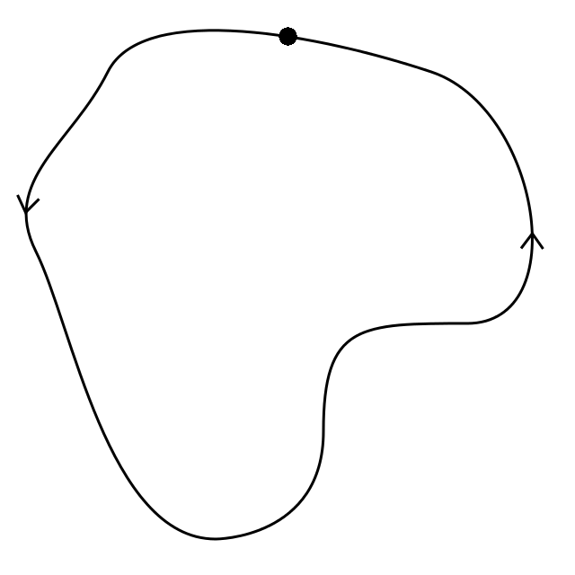
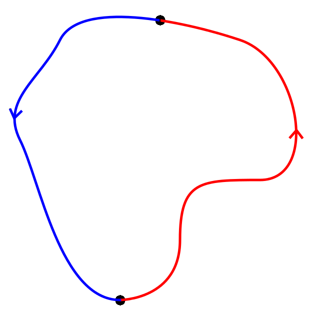
Figure 9. For two markings with associated basepoints and of a thin loop there exist representatives paths with sitting instants (shown on the right) (in red) and (in blue) such that (shown on the left) represents one marking and (shown in the middle) represents the other. Note that and are thinly homotopic. Therefore, without loss of generality, we can choose a single representative of a thin free loop with a decomposition as in the Lemma. We denote and Thus is one of or Note that and are thinly homotopic. For convenience, from now on we abuse notation often and do not distinguish between the actual paths versus the thin homotopy classes as elements of
By functoriality of the transport functor we have
(72) so that changes by conjugation in when the marking is changed.
- i)
- ii)
Suppose that is a morphism of transport functors. Then, for every thin path we have a commutative diagram
(73) which says
(74) If we restrict this to a thin marked loop with then
(75) so that again, changes under conjugation when the functor is changed to an isomorphic one.
- iii)
Suppose that another trivialization was chosen. Then following the comments after Remark 2.26, we can choose natural isomorphisms and resulting in a natural isomorphism This means every transport functor gets assigned a morphism of transport functors satisfying naturality. This means to every we have a morphism satisfying naturality, i.e. to every path the diagram
(76) commutes. In case is a thin loop at this gives
(77)
In conclusion, the answer to every one of the three questions is conjugation. This is what is called gauge covariance. To get something gauge invariant, we first denote the quotient map from to its conjugacy classes by where stands for the inner automorphisms of and the quotient is given by the conjugation action of on itself. All of the above considerations show that the following theorem holds.
Theorem 2.39.
Let be a smooth manifold, be a Lie group, a category, and suppose that is full and faithful. Let be a transport functor and a group-valued transport extraction. Let and be defined as above. Then the composition
| (78) |
is
- i)
independent of
- ii)
independent of the isomorphism class of
- iii)
and independent of the isomorphism class of
Notice that this theorem lets us make the following definition.
Definition 2.40.
Let be an isomorphism class of transport functors. The gauge invariant holonomy of is defined to be the map in the previous theorem, namely
| (79) |
where is a representative of is a group-valued transport extraction, and is a marking of thin loops in Let If is such that is a single element, we will say that is gauge invariant and abusively write instead of
3. Transport 2-functors and gauge invariant surface holonomy
In the present section, we review the basics of transport 2-functors and also provide some new and interesting results. As a preliminary, we briefly set our notation and review some facts about (strict) 2-groups and crossed modules. Then we split up the discussion into several parts and follow a similar pattern to the transport functor case. However, since we are now aware of what local triviality should mean, we skip the guess-work and head straight to the correct theory. We start with a Čech description of ordinary principal (strict) 2-group 2-bundles (without connection) in terms of smooth 2-functors. We then discuss how to add connection data by introducing transport functors, local triviality, and descent data. The discussion of the reconstruction functor is more involved, and because it is important for the calculation, we spend some time on it. Nevertheless, we skip some technical details (such as compositors and unifiers). Then we consider the differential cocycle data and discuss a formula for higher holonomy in terms of an iterated surface integral. We summarize the results as before. Sections 3.1 through 3.7 are a summary of [ScWa11], [ScWa], and [ScWa13].
Finally, in Section 3.8, we discuss some results on surface holonomy and its gauge covariance. We introduce a notion of -conjugacy classes for a 2-group in Definition 3.40 and prove in Theorem 3.41 that surface holonomy along spheres is well-defined in -conjugacy classes generalizing the reduced group of [ScWa13] (it is not yet known whether this generalization will work for more general surfaces). In the process, the procedure of group-valued transport extraction is categorified for the purposes of (i) proving this theorem and (ii) providing a functorial description for computing transport locally, which we utilize in Section 5.
We assume the reader is familiar with the basics of 2-categories. A review sufficient for most of our purposes can be found in Appendix A of [ScWa].
3.1. 2-group conventions
The theory of 2-groups is discussed in great detail in the article [BaLa04]. However, to simplify the discussion, we will define a (strict) 2-group as a strict one-object 2-groupoid, i.e. a strict 2-category with inverses for all 1- and 2-morphisms. Normally, one defines a 2-group as a groupal groupoid as in [BaLa04], but we find this unnecessary. However, to be consistent with notation in the literature, we will write our 2-groups as and use the notation where appropriate.
There is a 2-category of strict 2-groups denoted by - whose 1-morphisms and 2-morphisms are functors and natural transformations, respectively. It is useful to relate this higher-categorical definition to one involving ordinary groups. Although this is standard, we set the notation, which may differ from some authors.
Definition 3.1.
A crossed module is a quadruple of two groups, and and group homomorphisms and satisfying the two conditions
| (80) |
and
| (81) |
In this definition, is the automorphism group of The collection of crossed modules form the objects of a 2-category
Theorem 3.2.
The 2-categories and - are equivalent.
This theorem has been known for quite some time in several different forms. A simple place to start for this is in the article [BaHu11] with more information in [BaLa04].
Proof.
We only prove the equivalence at the level of objects and in only one direction. This will set up our conventions throughout the paper. Given a crossed module the associated 2-group is defined to have a single object as its set of 1-morphisms, and as its set of 2-morphisms. Composition of 1-morphisms is given by multiplication in The source and target maps of 2-morphisms are defined pictorially by
| (82) |
Vertical and horizontal compositions are defined by
| (83) |
and
| (84) |
respectively. When writing 2-group multiplication, we will always drop the composition symbol which is a common practice for ordinary group multiplication. ∎
The above proof sets up our convention for 2-group multiplication. Equation (82) shows that what’s needed to specify a 2-morphism is an element of the source of the 2-morphism, and an element of Thus, if the source is already known, the element in specifies the 2-morphism. Equation (83) defines vertical composition and equation (84) defines horizontal composition. Please be aware that different authors have different conventions (since the 2-categories and - are equivalent in many ways).
The following is a simple but important fact (which we use in studying gauge invariance, mainly Corollary 5.2).
Lemma 3.3.
Let be a crossed module. Then is a central subgroup of
Proof.
Let and Then
| (85) |
∎
Definition 3.4.
A Lie crossed module is a crossed module with and Lie groups and where and are smooth maps, where being smooth technically means that the adjoint map is smooth.
Definition 3.5.
A Lie 2-groupoid is a strict 2-category whose objects, 1-morphisms, and 2-morphisms are all smooth spaces and all structure maps are smooth. Furthermore, all 1- and 2-morphisms are invertible and the inversion maps are all smooth.
Definition 3.6.
A Lie 2-group is a Lie 2-groupoid with a single object.
Remark 3.7.
Lie crossed modules form the objects of a 2-category and Lie 2-groups form the objects of a 2-category. A similar proof shows that these 2-categories are also equivalent.
3.2. A Čech description of principal -2-bundles
Let be a Lie 2-group and denote the associated crossed module by Principal -2-bundles over a manifold can be described in terms of 2-functors using the Čech groupoid as well (this also comes from Remark II.13. of [Wo11]). However, since we are dealing with 2-categories we need to slightly modify the Čech groupoid of Definition 2.1. The way we do this is just by throwing on identity 2-morphisms. In other words, given an open cover of a 2-morphism from to exists only if and and in this case there is only the identity 2-morphism. Composition is uniquely defined by this. This defines the Čech 2-groupoid, also written as This is a Lie 2-groupoid.
Definition 3.8.
2-functors between Lie 2-groupoids are smooth if they assign data smoothly. Similarly, pseudonatural transformations and modifications are smooth when the assignments defining them are smooth.
Any smooth 2-functor gives the Čech cocycle data of a principal -2-bundle over subordinate to the cover To see this, simply recall what a 2-functor does (see Definition A.5. of [ScWa]). To each object in it assigns the single object in To each jump it assigns an element denoted by in such a way that we get a smooth 1-cochain as in Section 2.1. However, to each triple intersection which corresponds to the composition of with it assigns an element in such a way that we get a smooth 2-cochain
| (86) |
which says
| (87) |
The 2-functor satisfies an associativity condition which is translated into a condition on quadruple intersections giving a “cocycle condition”
| (88) |
where is short for etc. This condition says
| (89) |
which after multiplying out (using the rules of Section 3.1) and projecting both sides to gives
| (90) |
The 2-functor also assigns 0-cochains
| (91) |
which says
| (92) |
These satisfy two “degenerate” cocycle conditions on each double intersection of for the two ways one edge can be collapsed on the triangle. One is
| (93) |
which after multiplying out and projecting to says
| (94) |
The other cocycle condition is
| (95) |
which after multiplying out and projecting to says
| (96) |
Refinements and 1-morphisms between two such 2-functors is similar to the ordinary functor case from Section 2.1 but a bit more subtle due to modifications (which we won’t discuss now anyway). Let be another cover of with associated Čech 2-groupoid Let and be two smooth 2-functors. A 1-morphism from to consists of a common refinement of both and along with a smooth pseudo-natural transformation
| (97) |
By definition (see Definition A.6. in [ScWa]), to each object in such a pseudo-natural transformation gives a smooth function as before, but also to each jump in it gives another smooth function fitting in the diagram
| (98) |
which says that
| (99) |
The higher naturality conditions of a pseudo-natural transformation are given as follows. In general, to every 2-morphism, there is an associated naturality condition, but because the 2-morphisms in are all identities, this condition is vacuously true. To every pair of composable 1-morphisms and we get
| (100) |
Commutativity of this diagram says
| (101) |
which after equating both projections to gives
| (102) |
for all
Finally, to every object we get on each open set
| (103) |
where the back face of the cylinder is the identity 2-morphism This reads
| (104) |
which after projecting to says
| (105) |
Therefore, a 1-morphism of such principal 2-bundles as described above defines an equivalence of principal 2-bundles as described in [Wo11].
We won’t discuss 2-morphisms now because we will see that the above construction is a special case of the concept of limits of 2-categories in Section 3.7.
3.3. Local triviality of 2-functors
Just as transport functors describe parallel transport along paths, transport 2-functors describe parallel transport along paths and surfaces. They exhibit a formulation of a generalization of bundles with connection that describe such transport. We start by generalizing the thin path groupoid to the thin path 2-groupoid At this point, one should recall Definition 2.30 where bigons are introduced.
Definition 3.9.
Let be a smooth manifold. Two bigons and are said to be thinly homotopic if there exists a smooth map with the following two properties.
- i)
First, there exists an with such that
(106) - ii)
Second, the rank of is strictly less than 3 for all and is strictly less than 2 for all
In this case, is said to be a thin homotopy from to The set of equivalence classes of bigons under thin homotopy is denoted by Elements of are called thin bigons.
Definition 3.10.
Let be a smooth manifold. The thin path-2-groupoid is a 2-category defined as follows. The set of objects and 1-morphisms of coincide with that of The set of 2-morphisms of is Let be a thin bigon. The source and targets are defined by choosing a representative bigon and taking the thin homotopy equivalence classes of the paths and respectively. For a thin path the identity at is the thin homotopy class of the bigon
The various compositions in are the usual ones of composing paths and homotopies by either stacking squares vertically or horizontally and parametrizing via double speed vertically or horizontally, respectively. More concretely, given two vertically composable thin bigons55 5 To be absolutely clear, we write square brackets to denote the thin homotopy equivalence classes. After this definition, we will generally not do this, unless otherwise specified.
| (107) |
the vertical composition is given by first choosing representatives for the target of and for the source of Then, there exists a thin (rank strictly less than 2) homotopy Using this thin homotopy, the vertical composition is the thin homotopy class associated to the bigon
| (108) |
Given two horizontally composable thin bigons
| (109) |
the horizontal composition is given by the thin homotopy class associated to
| (110) |
All such compositions are well-defined, smooth, associative, have left and right units given by constant bigons for horizontal composition and paths viewed as bigons for vertical composition respectively, and satisfy the interchange law. is a Lie 2-groupoid since thin homotopy classes of bigons are invertible in both ways and the functions that assign every class to its vertical and horizontal inverses are both smooth.
Remark 3.11.
In the definition of vertical composition (108), we can always choose representatives of and so that and we can ignore for all practical purposes of this paper. Therefore, we will always write the vertical composition as
| (111) |
Definition 3.12.
Let be a Lie 2-groupoid, be a 2-category, a 2-functor, and a smooth manifold. Fix a surjective submersion A -local -trivialization of a 2-functor is a pair of a strict 2-functor and a pseudonatural equivalence
| (112) |
meaning that there exist a weak inverse along with modifications (see Definition A.8. in [ScWa]) and satisfying the zig-zag identities (see Definition 7. of [BaLa04] and particularly their discussion on string diagrams). The 2-groupoid is called the structure 2-groupoid for
2-functors equipped with -local -trivializations form the objects, written as triples of a 2-category denoted by
Definition 3.13.
A 1-morphism of -local -trivializations in is a pseudo-natural transformation A 2-morphism is a modification.
Definition 3.14.
Let be a Lie 2-groupoid, a 2-category, a 2-functor and a surjective submersion. A descent object is a quadruple consisting of a strict 2-functor a pseudonatural equivalence
| (113) |
and invertible modifications
| (114) |
and
| (115) |
These modifications must satisfy the coherence conditions which are explicitly given in Definition 2.2.1. of [ScWa] (in the examples of this current paper, the above modifications will actually be trivial and the coherence conditions will automatically be satisfied, which is why we leave them out).
Descent objects form the objects of a 2-category denoted by Morphisms and 2-morphisms are defined as follows.
Definition 3.15.
A descent 1-morphism from to is a pair with a pseudo-natural transformation and an invertible modification
| (116) |
These must satisfy certain identities explained in Definition 2.2.2. of [ScWa].
Definition 3.16.
Let and be two descent 1-morphisms from to A descent 2-morphism from to is a modification satisfying a certain identity explained in Definition 2.2.3. of [ScWa].
There is a 2-functor that extracts descent data from trivialization data. At the level of objects, this functor is defined as follows. Let be an object in For the quadruple take to be exactly the same. For take the composition coming from the composition in the diagram
| (117) |
just as before but this time is a weak (vertical) inverse to By definition should be a modification Using our definition of this means that we can break it down as follows
| (118) |
where all equalities hold by commutativity of certain diagrams and the leftover is specified by the following sequence of modifications
| (119) |
where is part of the pseudo-natural equivalence from and and is a left unifier.
Finally, by definition should be a modification Using our definition of we can break it down as follows
| (120) |
and such a modification can be achieved by
| (121) |
where is the other part of the pseudo-natural equivalence from and This indeed defines a descent object and that this assignment of descent data to trivialization data extends to a 2-functor to include 1-morphisms and 2-morphisms (see Lemma 2.3.1., Lemma 2.3.2., and Lemma 2.3.3. of [ScWa]).
Definition 3.17.
Let be a -local -trivialization of a 2-functor i.e. an object of The descent object associated to the -local -trivialization is A similar definition is made for 1- and 2-morphisms.
3.4. Transport 2-functors
We now wish to discuss smoothness for descent data. However, to do this is not so simple as it was for ordinary functors. We will have to make a detour to describe how to think of natural transformations as functors and modifications as natural transformations by altering the source and target categories. For the purposes of this document, we will make stricter assumptions than is done in [ScWa13] that are sufficient for our purposes and simplify several of the arguments and constructions.
Let and be two strict 2-categories. Let denote the category whose objects and morphisms are the objects and 1-morphisms of respectively. Because is strict, this defines a category. Let be the category whose objects are morphisms of The set of morphisms in from to are pairs of morphisms along with a 2-morphism as in the diagram
| (122) |
The composition is given by stacking
| (123) |
One can check that under our assumptions, this forms a category.
Notice that has a bit more structure. It also has a partially defined operation on objects and 1-morphisms given by “stacking vertically.” Suppose that and are two 1-morphisms in then one can compose them and this gives a partially defined associative and unital operation on objects of Similarly, given morphisms in which can be vertically stacked as in the diagram
| (124) |
This additional partially defined composition is written as in [ScWa13] so we stick with this notation.
Associated to a pseudo-natural transformation as in
| (125) |
is a functor defined by
| (126) |
on objects in i.e. objects in and
| (127) |
on morphisms in i.e. 1-morphisms in One can check this defines a functor.
Associated to a modification as in
| (128) |
is a natural transformation defined by
| (129) |
This defines a functor where is the category whose objects are pseudonatural transformations and morphisms are modifications while (between two ordinary categories and ) is the category whose objects are functors from to and whose morphisms are natural transformations.
Separately, notice also that if is a 2-functor then there is a functor defined by
| (130) |
on objects and
| (131) |
on morphisms.
Definition 3.18.
A descent object as in Definition 3.14 is said to be smooth if
- i)
the 2-functor is smooth,
- ii)
the functor is a transport functor with -structure, and
- iii)
the natural transformations and are morphisms between transport functors.
Smooth descent objects form the objects of a 2-category denoted by and form a sub-2-category of Smoothness of descent 1-morphisms and descent 2-morphisms is discussed in [ScWa13] following Definition 3.1.2.
Definition 3.19.
A -local -trivialization is said to be smooth if the associated descent object is smooth. The same can be said of 1-morphisms and 2-morphisms.
Smooth local trivializations, 1-morphisms, and 2-morphisms form a sub-2-category denoted by of Furthermore, restricts to an equivalence of 2-categories of smooth data (Lemma 3.2.3. of [ScWa13]).
After all this formalism, it should be more or less clear now what the definition of a transport 2-functor is by just abstracting what we did for the one-dimensional case (Definition 3.2.1. of [ScWa13]).
Definition 3.20.
Let be a Lie 2-groupoid, a 2-category, a 2-functor, and a smooth manifold. A transport 2-functor on with values in a 2-category and with -structure is a 2-functor such that there exists a surjective submersion and a smooth -local -trivialization
Transport 2-functors over with values in with -structure form the objects of a 2-category A 1-morphism of transport functors is a pseudo-natural transformation of 2-functors for which there exists a common surjective submersion and smooth -local -trivializations of both 2-functors so that the associated descent 1-morphism is smooth. A similar definition exists for 2-morphisms.
As a short summary, in the past two sections we introduced three categories for describing transport 2-functors. These were and The category was used to describe local triviality of transport 2-functors and their morphisms in We then constructed a 2-functor that allowed us to describe smoothness via the subcategory from which we defined
3.5. The reconstruction 2-functor: from local to global
The 2-functor is an equivalence of 2-categories (Proposition 4.1.1. of [ScWa]). To construct a (weak) inverse we need to enhance the Čech path groupoid so that it includes more data.
We do not require the full general definition of in Section 3.1 of [ScWa] for our purposes, but briefly the general definition is obtained by keeping the same objects and morphisms but replacing the relations that we imposed by 2-morphisms and setting relations on those. There are also additional 2-morphisms given by thin bigons, thin paths on intersections, and other formal 2-morphisms such as associators, unitors, and 2-morphisms relating the formal product to the usual composition of paths. We therefore warn the reader that although the following definition is not the same as that in [ScWa], we use their general results and theorems which in fact rely on their more general definition.
Definition 3.21.
Let be a smooth manifold and let be a surjective submersion. The Čech path 2-groupoid of is the 2-category whose set of objects and 1-morphisms are the objects and morphisms of respectively. The set of 2-morphisms are freely generated by
- i)
thin bigons in
- ii)
thin paths in with sitting instants thought of as 2-isomorphisms
(132) (one should think of this as weakening the first relation in Definition 2.20 of —see Figure 10 for a visualization of this),
Figure 10. Thinking in terms of an open cover as a submersion, condition ii) above says that if a thin path (with chosen representative) is in a double intersection, there is a relationship between going along the path first and then jumping versus jumping first and then going along the path. The two need not be equal. - iii)
points in thought of as 2-isomorphisms
(133) (one should think of this as weakening the second relation in Definition 2.20 of ),
- iv)
points in thought of as 2-isomorphisms ( is the formal identity)
(134) (one should think of this as weakening part of the third relation in Definition 2.20 of ),
- v)
and several other more technical generators that will not be discussed here.
There are several relations imposed on the set of 1-morphisms and 2-morphisms. We will not discuss any of them, and the reader is referred to Section 3.1 of [ScWa] for the details. As before, the compositions will be written with and will be drawn vertically or horizontally when dealing with 2-morphisms.
As before, we associate to every object in a functor defined as follows. It sends to thin paths in to and jumps to For the basic 2-morphisms, it makes the following assignments
| (135) |
for thin bigons in
| (136) |
for thin paths in
| (137) |
for points in and
| (138) |
for points in This defines a 2-functor at the level of objects. The rest of this 2-functor is defined in Proposition 3.3.2. of [ScWa].
There is a canonical projection functor defined in the same way as on the level of objects and morphisms. On the level of 2-morphisms, sends a thin bigon in to a the thin bigon in It sends a thin path in to the identity thin bigon (the vertical identity) in and it sends a point in to to the constant thin bigon at the point in Finally, it sends a point in to the constant thin bigon at the point in We now move on to defining, as before, a weak inverse of the canonical projection functor. To define we will constantly use the following important fact (Lemma 3.2.2. of [ScWa]).
Lemma 3.22.
Let be a thin path in and let and be two lifts of as 1-morphisms in (the existence follows from our choices above when we defined ). Then there exists a unique 2-isomorphism in such that
We will use this to define on thin bigons (we have already defined near (33) on objects and 1-morphisms). Let be any thin bigon in as in Figure 11.

As in the case of a path, because the domain is compact, there exists a decomposition of the bigon (we abuse notation and write to mean a bigon and its thin homotopy class relying on context to distinguish them) into smaller bigons as in Figure 12, each of which fits into an open set We use the same notation as before for our local sections.

Therefore, it suffices to define for a single one of the associated thin bigons provided that we match up all sources and targets for the individual ones. Denote the thin bigon by
| (139) |
Then the image of this under is defined as the composition
| (140) |
In other words, we have lifted using the section but to make sure that this image matches up with how was already defined on objects and 1-morphisms, we use the obvious jumps and the unique 2-isomorphisms from Lemma 3.22 to match everything (these are the unlabeled 1-morphisms and 2-morphisms). The image of the entire thin bigon is then defined by vertical and horizontal compositions of all the so that respects compositions.
The 2-functor is a weak inverse to as in the case for the path groupoid (Proposition 3.2.1. of [ScWa]). However, a weak inverse in 2-category theory in this case means that there exists a pseudo-natural equivalence since This means there exists a weak inverse to which is written as “Weak” means that there are invertible modifications and that satisfy the zig-zag identities. The details are irrelevant for our purposes but can be found in Section 3.2 of [ScWa]. An important consequence of being a weak inverse to is the following (general categorical) fact reproduced here for convenience (Corollary 3.2.5. of [ScWa]).
Corollary 3.23.
Any two weak inverses of are pseudo-naturally equivalent.
We can define such a pseudo-natural equivalence by the following assignment the jump from to and the unique 2-isomorphism specified by Lemma 3.22. We will exploit this fact when discussing examples of higher holonomy in Section 5.
As before, the 2-functor induces a 2-functor the pullback along Similarly, is defined as the composition in the diagram
| (141) |
As before, the image of under lands in and the definition is the same as it was before, only this time is a pseudo-natural equivalence between 2-functors between 2-categories.
As a short summary, in this section we introduced a weak inverse functor for by using the 2-groupoid associated to the surjective submersion to lift points, thin paths, and thin bigons in to points, thin paths and/or jumps, and thin bigons and/or jumps in respectively.
3.6. Differential cocycle data
In this section, we will give a brief review of an equivalence between differential forms and smooth 2-functors following Section 2 of [ScWa11]. This will allow us to describe parallel transport locally in terms of differential cocycle data. We will leave out several proofs but will provide pictures that we find illustrate the necessary ideas behind the statements. We first remind the reader of the “Lie algebra” of a Lie crossed module.
Given a Lie crossed module (recall Definition 3.1) there is an associated differential Lie crossed module where is the differential of is the differential of the associated action (given the same name) (“Der” stands for derivations). The differential Lie crossed module data satisfy
| (142) |
and
| (143) |
for all and
Note that by restricting the action to for any and differentiating with respect to the second coordinate, we obtain a Lie algebra homomorphism Both and are important for understanding the differential cocycle data of Section 3.6. A more thorough review can be found in [BaHu11].
3.6.1. From 2-functors to 2-forms
Let be a Lie 2-group and its corresponding crossed module. Given a strict smooth 2-functor we will obtain differential forms and These will form the objects of a 2-category By our previous discussion and since our 2-categories and are strict and the 2-functor is strict, the restriction of to is smooth. Therefore, we obtain a differential form by the results of Section 2.6. To obtain the differential form we will “differentiate” the composition
| (144) |
where is the projection onto the factor and is restricted to 2-morphisms.
Infinitesimally, a bigon is determined by a point and the two tangent vectors that begin to span it. Therefore, let and and let be a smooth map such that
| (145) |
Let be the (smooth) map that sends to the thin homotopy class of the bigon in Figure 13. This is unambiguously defined after modding out by thin homotopy because a thin bigon in is determined by its source and target thin paths in

Then we use this to define a smooth map by the composition of smooth maps
| (146) |
This gives an element of the Lie algebra by taking derivatives
| (147) |
Furthermore, this element is independent of the choice of provided that equation (145) still holds. In fact, we get a smooth differential form
Now let be a thin bigon between two thin paths. The source-target matching condition, which says implies
| (148) |
All of these claims are proved in Section 2.2.1 of [ScWa11].
3.6.2. From 2-forms to 2-functors
Starting with a -valued 1-form on and a -valued 2-form on we want to define a smooth functor From Section 2.6.2, we have already defined the functor at the level of objects and thin paths. What remains is to define To do this, we will define a function on bigons in (we do not mod out by thin homotopy). Given a bigon we can pull back the 1-form and the 2-form to obtaining and
To define we first introduce an -valued 1-form obtained by integrating over one of the directions for the bigon. It is defined by
| (149) |
where is defined to be the straight vertical path from to in as in Figure 14. Note that in expression (149), it is assumed that refers to the thin homotopy class of the path (otherwise, applying the function would not make sense). Therefore, the parametrization of is irrelevant.

Besides the path-ordered integral expression from the term the expression for is an ordinary integral. Also note that depends on In particular, it is not invariant under thin homotopy.
Remark 3.24.
Incidentally, although Schreiber and Waldorf in [ScWa11] made their own arguments for how to obtain such a formula for this formula appears in a special case as early as 1977 in the work of Goddard, Nuyts, and Olive on magnetic monopoles [GoNuOl77] on the right-hand side of equation (2.9) and it may have been known earlier [Ch75]. The special case [GoNuOl77] considered is the case of the crossed module with being the ordinary conjugation action.
Finally, to every bigon we define
| (150) |
In Figure 15, this integral is schematically drawn as a power series of graphs with marked points and paths analogous to Figure 5. Each of the paths drawn has a path-ordered integral expression attached to it, and therefore each expression has an additional power series of the form we discussed for the ordinary path-ordered integral.
Definition 3.25.
The group element is called the surface transport associated to the bigon and the differential forms and
only depends on the thin homotopy class of and therefore factors through a smooth map on thin homotopy classes of paths. This map together with define a strict smooth 2-functor (Proposition 2.17. of [ScWa11]).
Remark 3.26.
Historically, understanding the appropriate generalization of the path-ordered integral to surfaces was a difficult task. It was not obvious which formulas were correct or even what the criteria for correctness should be. The language of functors allows one to make this precise. The criteria for correctness is that surface holonomy should be expressed in terms of a transport 2-functor. Any formula that satisfies these functorial properties, has the local constraint given by equation (148), and changes appropriately under gauge transformations (which we have so far only discussed globally but will discuss differentially soon), can be rightfully called surface transport. The specific formula in equation (150) is only one such formula that works. However, there could be many other, potentially simpler formulas, that also describe 2-holonomy. In Section 4 for instance, we prove that for certain structure 2-groups, the formula (150) agrees with one that is easily computable in terms of homotopy classes of paths.
3.6.3. Local differential cocycles for transport 2-functors
By similar considerations to the previous sections, we can differentiate transport functors and use their properties to obtain relations among all the differential data. All the information in this section is discussed in more detail in [ScWa13]. In particular, the functions, differential forms, and their relations are all derived. We merely reproduce the results here for use in later calculations.
Definition 3.27.
Let be the category defined as follows. An object of is a pair of a 1-form and a 2-form satisfying
| (151) |
A 1-morphism from to is a pair of a smooth map and a 1-form satisfying
| (152) |
and
| (153) |
The composition is defined by
| (154) |
A 2-morphism from to which are both 1-morphisms from to is a smooth map satisfying
| (155) |
and
| (156) |
The vertical composition is defined by
| (157) |
The horizontal composition is defined by
| (158) |
As in Section 2.6.3, these arguments define 2-functors
| (159) |
which turn out to be strict inverses of each other (Theorem 2.21 of [ScWa11]).
As before, this was for globally defined differential data corresponding to globally trivial transport 2-functors. Transport 2-functors on are not necessarily of this type, but they are locally trivializable via some surjective submersion and a -local -trivialization. By similar arguments to the discussion in Section 2.6.3, we are led to the following, rather long and complicated, definition.
Definition 3.28.
Let be a surjective submersion. Define the 2-category of differential cocycles subordinate to as follows. An object of is a tuple where is an object in is a 1-morphism from to in is a 2-morphism from to in and is a 2-morphism from to A 1-morphism from to is tuple where is a 1-morphism from to in and is a 2-morphism from to in A 2-morphism from to is a 2-morphism from to in
The above generalizations produce functors
| (160) |
exhibiting an equivalence of 2-categories whenever is an equivalence.
3.7. Direct limits
In this section, we get rid of the dependence on the surjective submersion in the categories introduced in the prequel. Several of our 2-categories depended on the choice of a surjective submersion. These 2-categories were and Changing the surjective submersion gives a collection of 2-categories dependent on this surjective submersion. One can take a limit over the collection of surjective submersions in this case. This will be a slight generalization of what was done in Section 2.7. However, there are subtle issues in terms of defining the many compositions.
The general construction is done as follows. Let be a family of 2-categories parametrized by surjective submersions and let be a family of 2-functors for every refinement of satisfying the condition that for any iterated refinement and of then In this case, an object of is given by a pair of a surjective submersion and an object of A 1-morphism from to consists of a common refinement
| (161) |
together with a 1-morphism in It is written as a pair The composition
| (162) |
consists of the pullback refinement
| (163) |
along with the composition A 2-morphism from to consists of an equivalence class of pairs where is a common refinement of and as in the following diagram
| (164) |
and is a 2-morphism Two such pairs and are equivalent if they agree on the pullback.
After getting rid of the specific choices of the surjective submersions, we can take the limits of all the categories we have introduced. We make the following notation, slightly differing from that of [ScWa13]:
| (165) | ||||
| (166) | ||||
| (167) |
Then from our previous discussions, we collect the functors we have introduced relating all these categories to after taking such limits over surjective submersions:
| (168) |
Under the conditions that is an equivalence of categories, all of the above 2-functors are equivalence pairs. Without the smoothness assumptions, a simpler version of some of these equivalences is proven in Proposition 4.2.1. and Theorem 4.2.2. of [ScWa] while the equivalences in (168) are proven in Theorem 3.2.2., Lemma 3.2.3., and Lemma 3.2.4. of [ScWa13]. Completely analogous versions of comments regarding the assumptions on made before (59) apply here as well.
3.8. Surface transport, 2-holonomy, and gauge invariance
In Section 2.8, we described a procedure that began with a transport functor and produced a group-valued parallel transport operator for thin loops with markings. We discovered that the value of holonomy changed by conjugation depending on the markings for the loops, the choice of a local trivialization procedure, and by using an isomorphic transport functor. In this section, we will analyze holonomy along surfaces in an analogous manner. The main difference is that bigons have source and target paths so that a closed surface has a marking of one lower dimension, and is therefore not in general just a point as it was for loops. For the examples we give later in this paper, we specialize to spheres with a point marking. Such a surface is depicted as a bigon from the constant loop at a point to itself (see Figure 16 below and [HoTs93]).

However, a sphere can be more generally described as a bigon from a loop to itself, so we analyze parallel transport for such bigons to cover these extra cases. This analysis is completely independent of what types of Lie 2-groups we use. For simplicity, we assume that is a full and faithful 2-functor. This will differ from the presentation in Section 5 of [ScWa13], where surface holonomy was defined using the reduced 2-group. We will not be making this restriction.
Definition 3.29.
A 2-group-valued transport extraction is a composition of functors (starting at the left and moving clockwise)
| (169) |
We write the composition (169) as By the reconstruction procedure of Section 3.5, assigns -valued elements to thin paths for every transport functor as well as -valued elements to thin bigons (more on this below). Technically, thin bigons will be assigned elements in but as is discussed in Section 3.1, particularly after the proof of Theorem 3.2, such elements are completely determined by their source, an element of and their projection in will also assign -valued and -valued gauge transformations for every 1-morphism of transport functors. In addition, will assign -valued 2-gauge transformations for every 2-morphism A pseudo-natural equivalence describes how to relate the transport functor to the locally trivialized one. Although modifications of pseudo-natural transformations are allowed, we will not analyze them in this paper. Such modifications are to be interpreted as relating the two different ways of choosing the pseudo-natural transformations that relate the transport functor to the locally trivialized one.
Just as before, we briefly review what the composition of 2-functors defining are. For a transport 2-functor we choose a local trivialization Then we extract the local descent object Then, we reconstruct a transport 2-functor and then forget the trivialization data keeping just the 2-functor The resulting transport 2-functor, written as is defined by (see Section 3.5)
| (170) |
Points in get sent to by construction. Because is full and faithful, the 1-morphisms determine unique elements of Similarly, the 2-morphisms determine unique elements in
The interested reader can explicitly define the compositor and the unitor for the 2-functor We won’t need the precise details for our analysis when studying surface holonomy. All we need to know is that the 2-functors defining are (weakly) invertible.
We’d like to restrict surface holonomy to thin homotopy classes of marked spheres for the purpose of this paper (in general, one would like to restrict to the more general space of thin homotopy classes of marked closed surfaces) and eventually thin free spheres. First we make a definition of the thin marked sphere space, which should be thought of as analogous to the thin marked loop space.
Definition 3.30.
The marked sphere space of is the set
| (171) |
equipped with the subspace smooth structure. Elements of are called marked spheres. Similarly, the thin marked sphere space of is the smooth space
| (172) |
Elements of are called thin marked spheres.
Remark 3.31.
Note that elements of need not look like embedded spheres in Indeed, they might look like pinched croissants as Figure 17 indicates (or worse). This won’t matter in any of our calculations or proofs.

Definition 3.32.
The -2-holonomy of , written as is defined as the projection to of the restriction of parallel transport of a transport 2-functor to the thin marked sphere space of :
| (173) |
Remark 3.33.
Note that is the same notation used for thin loops with values in This should cause no confusion because thin loops are always written using lower case Greek letters such as etc. while thin spheres are written using upper case Greek letters such as etc.
We now pose three questions analogous to those for 1-holonomy.
- i)
How does depend on the choice of a thin marked sphere? Namely, suppose that two thin marked spheres and with possibly different markings, are thinly homotopic without preserving the marking (see Definition 3.34). Then, how is related to ?
- ii)
How does depend on ? Namely, suppose that is a morphism of transport functors. How is related to in terms of ?
- iii)
How does depend on the choice of trivialization? Namely, suppose that is another trivialization. Then how is related to ?
Due to the fact that we are restricting ourselves to marked spheres instead of arbitrary surfaces, the answer will be closely related to the 1-holonomy case and will be given by a generalized version of conjugation. As before, we need to define what we mean by thin free sphere space and then we’ll proceed to answer the above questions. Denote the smooth space of spheres in by
Definition 3.34.
Two smooth spheres and in are thinly homotopic if there exists a smooth map such that
- i)
there exists an with for and for and for all and
- ii)
the smooth map has rank
The space of equivalences classes is denoted by and is called the thin free sphere space of . Elements of are called thin spheres.
Definition 3.35.
Define a function by sending a marked sphere to the associated smooth map obtained from identifying the top and bottom of the second interval and then pinching the two ends (see Figure 18). is called the forgetful map.

Lemma 3.36.
There exists a unique map such that the diagram
| (174) |
commutes (the horizontal arrows are the projections onto thin homotopy classes).
Proof.
The proof is analogous to the case of loops. One chooses a representative, applies and then projects. The map is well-defined by the thin homotopy equivalence relation on ∎
Note that there is also a function given by evaluating a thin marked sphere at its source/target. This function forgets the sphere and remembers only the source thin marked loop.
Definition 3.37.
A marking of thin spheres is a section of
Lemma 3.38.
A marking of thin spheres exists.
Proof.
Let be a thin sphere and choose representative in Pick a point on the equator viewed as a loop The image of under defines a loop, where There exists a thin homotopy from to a smooth map such that the family of loops in Figure 19 on the domain of define a marked sphere Projecting to thin marked spheres defines To see that this is well-defined, let be another representative. Then there exists a thin unmarked homotopy Composing this with the thin homotopy gives By the thin homotopy equivalence relation on this defines a section of ∎

We now proceed to answering the above questions in order.
- i)
Let be two markings for thin spheres in Let be a thin sphere and let with be a representative of and with be a representative of Note that these representatives need not have associated marked loops that lie on some common image. Figure 20 depicts such a possible situation.

Figure 20. Two different representatives (the ‘inner’ sphere in green extending left) and (the ‘outer’ sphere in purple extending right) of two markings of a thin sphere are shown. The extensions do not enclose any volume so that both spheres are thinly homotopic. Their respective sources are and neither of which lie on the other’s image. Compare this to Figure 23 where the two marked loops do lie on a common sphere. As in the case of loops, we can use thin homotopy to draw both marked loops on the same sphere (a more precise statement will be given shortly). First notice that there is a thin homotopy with for and for for some Such a homotopy allows us to choose a sphere a path and three bigons and with the following properties. First can be expressed as either of the compositions
(175) (in either order vertically). Second, the composition of bigons
(176) is thinly homotopic to preserving the marked loop Third, the composition of bigons
(177) is thinly homotopic to preserving the marked loop This is depicted in Figures 21 and 22.

Figure 21. The domain of the homotopy is drawn as a solid ball with a smaller solid ball removed from the center. It depicts as the inner sphere and as the outer sphere. The marked loop of is drawn on the northern hemisphere while the marked loop of is drawn on the southern hemisphere (by a thin homotopy, one can always position the marked loops in this way). The homotopy allows us to choose a sphere drawn somewhat in the middle (in orange), that contains both based loops and and is thinly homotopic to both and As a result, there exists a path on We continue this analysis in Figure 22. 


Figure 22. From the sphere in Figure 21, the top cap defines a bigon drawn on the left in this figure. The path in Figure 21 defines a bigon drawn in the middle of this figure. The bottom cap defines a bigon drawn on the right. These last two equations let us write the bigon in terms of and vice versa. In fact, we have
(178) up to thin homotopy preserving the marked loop There is also a similar expression for preserving the marked loop
The above argument says that given two marked spheres, with possibly different markings, that are thinly homotopic without preserving the markings, one can always choose a representative of such a thin sphere in with two marked loops so that the associated two marked spheres (coming from starting at either marking) are thinly homotopic to the original two with a thin homotopy that preserves the marking. More precisely, we proved the following.
Lemma 3.39.
Let be two markings. Let be a thin sphere in and write for and for Then, there exists representatives and of and respectively, a path with sitting instants and three bigons and such that the following three properties hold (see Figure 23).
- i)
The vertical composition of and in the order given (or a cyclic permutation of this order) and forgetting the marking is a representative of
- ii)
is a representative of as a bigon.
- iii)
is a representative of as a bigon.


Figure 23. For every thin sphere and two markings, there exists a representative with a decomposition as in Lemma 3.39. On the left is a bigon with The shaded region depicts the surface swept out between and some small In the middle is another bigon with and a path with sitting instants. On the right is a bigon relating the two marked loops as in (180). Therefore, without loss of generality, we can choose a single representative of a thin free sphere with a decomposition as in the Lemma. We use to denote the bigon in ii) of Lemma 3.39 and to denote the bigon in iii). The two are related by
(179) i.e.
(180) By functoriality of the transport 2-functor we have
(181) where is a combination of compositors and associators. Writing out this composition in the 2-group gives
(182) Multiplying these results out using the rules of 2-group multiplication (see equations (83) and (84)) and taking the component gives
(183) This result says that the 2-holonomy changes by -conjugation under a change of marking for a thin sphere.
- i)
- ii)
Now suppose that is a 1-morphism of transport 2-functors. Then, for every thin path we have a 2-isomorphism (remember that and for all )
(184) satisfying the condition that for any thin bigon with another path, the diagram
(185) commutes. In this diagram, the in the back is not shown. This diagram commuting means that
(186) and writing this out using group elements gives
(187) which after evaluating both sides and projecting to yields
(188) Solving for gives
(189) Now, after specializing to the case where the source and targets of are all the same, i.e. and so that we are comparing this transport along thin marked spheres, this reduces to
(190) This says that when restricted to thin marked spheres changes under -conjugation when the functor is changed to a gauge equivalent one
- iii)
Suppose that another 2-group transport extraction procedure was chosen. Any two such procedures are pseudo-naturally equivalent, i.e. if was another such choice, then there exists a weakly invertible pseudonatural transformation This follows from the fact that each 2-functor in the composition of 2-functors that define is an equivalence of 2-categories and weak inverses are unique up to pseudo-natural equivalences. Therefore, for every transport 2-functor we have a 1-morphism of transport functors Of course, we also have a map assigning to every 1-morphism of transport functors a 2-morphism satisfying naturality, but we will not need this fact for the following observation because we are dealing with strict Lie 2-groups. The 1-morphism of transport functors assigns to every point a morphism and to every path a 2-isomorphism
(191) satisfying the condition that for a thin bigon between two thin paths the diagram
(192) commutes. This result is very similar to the previous one and is given by
(193) which is again just -conjugation.
In conclusion, when restricted to a sphere, 2-holonomy changes under -conjugation in each of the three situations described above. This should therefore also be called gauge covariance as in the case for loops. This motivates the following definition.
Definition 3.40.
Let be a crossed module. The -conjugacy classes in , denoted by is defined to be the quotient of under the equivalence relation
| (194) |
Denote the quotient map by
As before, we have a similar theorem for gauge-invariance of 2-holonomy.
Theorem 3.41.
Let be a smooth manifold, a Lie 2-group, a 2-category, and suppose that is a full and faithful 2-functor. Let be a transport 2-functor and a 2-group-valued transport extraction. Let and be defined as above. Then the composition
| (195) |
is
- i)
independent of
- ii)
independent of the equivalence class of
- iii)
and independent of the equivalence class of
This theorem lets us make the following definition.
Definition 3.42.
Let be an equivalence class of transport 2-functors. The gauge invariant 2-holonomy of is defined to be the smooth map in the previous theorem, namely
| (196) |
where is a representative of is a group-valued transport extraction, and is a marking for thin spheres in Let If is such that is a single element, we will say that is gauge invariant and abusively write instead of
Remark 3.43.
We now compare this result to that in [ScWa13], where the reduced group associated to a 2-group was introduced in order to obtain a well-defined 2-holonomy independent of the marking as well as the representative of the transport functor used.
Definition 3.44.
Let be a 2-group with associated crossed module The reduced group of is where i.e. the subgroup of generated by elements of the form
The analogue of the reduced 2-group in the case of ordinary holonomy for principal bundles with connection is the abelianization of Recall, is a normal subgroup, called the commutator subgroup, of so the quotient is an abelian group, in fact in a universal sense.
Lemma 3.45.
Let be a group, its commutator subgroup, and conjugacy classes in The map given by taking a conjugacy class choosing a representative, and projecting to the quotient is
- i)
well-defined,
- ii)
surjective,
- iii)
and need not be injective in general.
Proof.
- i)
The map is well-defined because if was another representative of then there would be a such that and under the quotient map, the difference between and is
- ii)
Since is surjective, and the map defined by choosing a representative is well-defined, the map is surjective.
- iii)
To see why the map is, in general, not injective, consider the following example [DuFo04]. Let be the symmetric group on letters, i.e. it is the permutation group of elements. Let be the alternating group on letters. This group is defined as the kernel of the homomorphism given by taking the sign of the permutation. It turns out this kernel is also the commutator subgroup of Furthermore, its index is On the other hand, let’s compute the conjugacy classes of for some small The simplest case actually suffices, although we’ll quote some results for higher to indicate that the difference between conjugacy classes and abelianization gets bigger. For the set of conjugacy classes in is given by the following elements. The identity element, written as is in its own class. The elements and are in their own class. Finally, the elements and are in their own class. Therefore, the set of conjugacy classes for is given by a 3-element set whereas the abelianization is a 2-element group. For the set of conjugacy classes is a set of 5 elements. For the set of conjugacy classes is a set of 7 elements. The abelianization, however, is always of order 2.
∎
Therefore, conjugacy classes contain at least as much information about ordinary holonomy as do elements of the abelianization, and they are exactly the elements needed to define holonomy in a gauge invariant way due to Theorem 2.39.
In a similar way, the reduced group of a 2-group is analogous to the abelianization and does not contain the full information of 2-holonomy in general. One needs an analogue of conjugacy classes for 2-holonomy. The candidate, for spheres at least, is -conjugacy classes, In fact, we have a similar fact concerning -conjugacy classes and the reduced group.
Lemma 3.46.
Let be a crossed module, the associated 2-group, the reduced group of and the -conjugacy classes in . The map given by taking a conjugacy class choosing a representative, and projecting to the quotient is
- i)
well-defined,
- ii)
surjective,
- iii)
and need not be injective in general.
Proof.
- i)
Let and be two representatives. Then there exists a such that and so the difference between and is
- ii)
Since is surjective, and the map defined by choosing a representative is well-defined, the map is surjective.
- iii)
To see why the map is, in general, not injective, consider the special case where and is the ordinary conjugation. Then this case reduces to the previous case of Lemma 3.45.
Although the previous example suffices to show why -conjugacy classes contain more information than the reduced group in general, holonomy along spheres takes values in by the source-target matching condition. Therefore, it is also important to find an example of a crossed module such that and the map is not injective.
Take the (additive) cyclic group of order where is prime. Set the automorphism group of Let be the trivial map and be the identity map. defines a crossed module.
Every element of is of the form with and is determined by where it sends the generator: For this proof, denote the -conjugacy class of an element by For all so that is fixed under the action. However, since the set of -conjugacy classes of is which is just a 2-element set. However, the reduced group is trivial. To see this, consider generators of which are of the form with and Set and Then Therefore, the generator of is in the subgroup which means Thus
∎
In this case, one can make sense of gauge-invariant quantities coming from 2-holonomy without passing to the reduced group as is done in [ScWa13]. In the case of the examples considered in Section 5, one even gets a fixed point under the action, in which case one does not need to pass to the -conjugacy classes.
Definition 3.47.
Let be a crossed module. Denote the fixed points of under the action by
| (197) |
Lemma 3.48.
In the notation of Definition 3.47, is a central subgroup of
Proof.
Let Then
| (198) |
for all Thus, is closed. for all says Let then showing that Finally, is central because
| (199) |
for all and ∎
This will have physical relevance when discussing monopoles, which, as we will show, take values in
4. The path-curvature 2-functor associated to a transport functor
In this section, given a principal -bundle with connection and a choice of a subgroup of we construct a principal 2-bundle with connection whose structure 2-group is a covering 2-group obtained from and the subgroup of This assignment is functorial. We describe it on all levels introduced in the review, namely as a globally defined transport functor, in terms of descent data, and via differential cocycle data. These constructions respect all of the functors relating these different levels.
4.1. The path-curvature 2-functor
The transport 2-functor defined later in this section is motivated by the study of magnetic monopoles in gauge theories as described in [HoTs93]. Some of the earlier accounts of similar descriptions can be found in the work of Wu and Yang in [WuYa75] under the name ‘total circuit’ and also in the work of Goddard, Nuyts, and Olive in [GoNuOl77]. Of course, several others worked on understanding the “topological quantum number” due to a magnetic charge in terms of just the magnetic charge alone, but the three references mentioned are the ones that have influenced us. We argue in Section 5 that in the case where the base space is a 3-manifold, this transport 2-functor has 2-holonomy along a sphere which is given by the magnetic flux through that sphere. Therefore, we give a mathematically rigorous description of non-abelian flux for magnetic monopoles in a non-abelian gauge theory. A more detailed description of the physics will be given in that section, but first we explain the mathematical structure.
The starting data consist of (i) a principal -bundle, where is a connected Lie group, with connection over a smooth manifold and (ii) a subgroup of By the main theorem of [ScWa09], the first part of the data corresponds to a transport functor with structure. From this data, we will construct a transport 2-functor which we call the path-curvature 2-functor. We will discuss two interesting cases for the choice of although other choices are important for applications in physics so we keep this generality for future applications. When the path-curvature 2-functor coincides with the curvature 2-functor of Schreiber and Waldorf [ScWa13]. The choice the trivial group, will be more appropriate in the context of gauge theory and computing invariants. This is the case we focus on for all our computations in Section 5.
To set up this example, we introduce the following Lie 2-group associated to any connected Lie group Let be the universal over of (we will describe what happens for arbitrary covers later) and denote the covering map by An explicit construction of in terms of homotopy classes of paths will be useful for our purposes
| (200) |
where if and there exists a homotopy relative the endpoints. naturally acquires a topology as the quotient space of a subspace of paths. Denote the equivalence class representing a path with square brackets as in or where it is understood that takes values in The multiplication in is defined by choosing representatives and multiplying them pointwise (later we will show that this multiplication can be described in another way that is sometimes more convenient for our examples). Let be the conjugation map meaning
| (201) |
where the concatenation means multiplication in Define to be evaluation at the endpoint,
| (202) |
Proposition 4.1.
defined in the previous paragraph is a Lie crossed module.
Proof.
It is useful to recall the definition of a crossed module (Definition 3.1) at this point. Since the equivalence relation involves homotopy relative endpoints, is well-defined. is well-defined because implies The topological space has a unique smooth structure making the map a homomorphism and a smooth covering map, i.e. a smooth surjective submersion with the property that for every there exists an open neighborhood containing such that each component of maps to diffeomorphically. This follows from some basic differential topology (see for example Theorem 2.13 of [Le03]). Conjugation in is a smooth map, and because is well-defined, is therefore smooth. The only things left to check are the crossed module identities. First, let and let and be representatives of and respectively. Then the map
| (203) |
is a homotopy (relative endpoints) from the path (when ) to the path (when ). Therefore,
| (204) |
which is the first identity (80). For the second identity, let and with a representative Then
| (205) |
which proves the other identity (81). ∎
Definition 4.2.
The Lie crossed module defined above is called the universal cover crossed module associated to a Lie group The associated Lie 2-group, denoted by is called the universal cover 2-group associated to the Lie group
In fact, the only way to give a smooth covering map a Lie crossed module structure is the way we have done so above. This follows from the following Lemma.
Lemma 4.3.
Let be a crossed module (not necessarily Lie) with a surjective homomorphism. Then is conjugation in by a choice of lift, namely
| (206) |
for some with
Proof.
First we prove that conjugating by a lift is well-defined. Let be another lift with Then
| (207) |
since is a homomorphism. The claim that for a choice of lift of then follows from the identity (80) since for some because is surjective and a lift always exists. ∎
Lemma 4.4.
Let be a Lie crossed module with a smooth covering map. Then is conjugation in by a choice of lift, namely
| (208) |
for some with
Proof.
The claim holds even if is just surjective. The proof follows from Lemma 4.3 viewing and as groups (ignoring smooth structure) and using the identity for some lift of ∎
Given any subgroup we can construct another Lie 2-group in a similar way but by using a different equivalence relation. Define
| (209) |
where if and where denotes the reverse path and we use a vertical representation for the concatenation of paths in this context
| (210) |
Definition 4.5.
An equivalence class of paths under the equivalence relation in equation (209) will be denoted by or and will be called an -class.
Proposition 4.6.
Let be a connected Lie group, a subgroup, and as in (209). Then for the function given by
| (211) |
with a choice of a representative of is a well-defined homomorphism. Furthermore, has a unique smooth structure so that is a smooth covering map. Finally, with defined by
| (212) |
is a Lie crossed module.
Proof.
is well-defined by definition of the equivalence relation is a homomorphism because has a natural topology coming from the quotient space of a subspace of paths in Because is abelian, the conjugacy class of is itself. Therefore, by a standard theorem of constructing covering spaces (see for instance Chapter 3 of [Ma99]) is a covering map. By another standard result in differential topology (see Proposition 2.12 of [Le03]), there is a unique smooth structure on making a smooth covering map. By construction, has a continuous multiplication making it a topological group. The only things left to prove is that the multiplication and inversion maps in are smooth. This can be done locally using the smoothness of multiplication and inversion in and the fact that is a local diffeomorphism. Therefore, is a Lie group. Since is smooth, is a Lie group homomorphism. is a well-defined group homomorphism for all because it can be described as conjugation. It is smooth because for any there exists an open neighborhood around a diffeomorphism with a component of so that coincides with conjugation by by the proof of Lemma 4.4. Since conjugation is smooth for any Lie group, is smooth. Therefore, is a Lie crossed module. ∎
Note: We use the same notation and for the maps instead of and since we typically fix in any given context.
Definition 4.7.
Let be a Lie group and a subgroup of Then as described in Proposition 4.6 is called the -cover crossed module of Its associated 2-group is called the -covering 2-group and is denoted by We sometimes abusively say covering crossed module or covering 2-group without referring to explicitly.
Let be a subgroup of the fundamental group of a Lie group We will now construct a 2-category whose underlying 1-category (see the beginning of Section 3.4) is Although the category is not a Lie groupoid, notice that the set of morphisms between any two -torsors is isomorphic to and therefore has a unique smooth structure. Furthermore, the composition is a smooth map and is modeled by the group multiplication map By this we mean that by choosing basepoints and in -Torsors and respectively, the composition
| (213) |
agrees with the multiplication under the isomorphisms specified by the choice of basepoints. Therefore, the composition is smooth. Thus, is enriched in smooth manifolds. Using this fact, we can extend to an interesting 2-category in a non-trivial way.
Let and be two -torsors and let be two morphisms of -torsors. We define the set of 2-morphisms from to , drawn as
| (214) |
to be the set of -classes of paths from to in - This means the following.
Definition 4.8.
Let be a subgroup. Two paths and in - drawn as
| (215) |
are said to be -equivalent if under the diffeomorphism defined by
| (216) |
the homotopy class of the loop which gets sent to an element of under this diffeomorphism, is an element of The class associated to is called an -class of paths and is denoted by
The choice of diffeomorphism (216) where is merely for convenience. In particular, the element is independent of this diffeomorphism. To see this, if any other diffeomorphism was chosen, say sending some other morphism to then there exists a unique so that so that In this case, one gets a loop based at To get one at we merely multiply by to obtain a loop based at This loop is exactly the same as under the diffeomorphism defined by Therefore, the homotopy class is independent of the diffeomorphism chosen.
Vertical composition is defined on representatives as concatenation of paths. Horizontal composition can be defined using the multiplication. More explicitly, for two composable 2-morphisms as in
| (217) |
choose representatives of such paths so that and with and Define the horizontal composition to be the -class of the path defined by
| (218) |
where the composition on the right-hand-side is the usual composition of morphisms in We check that horizontal composition is well-defined. Suppose that and We must show that i.e.
| (219) |
but a representative of this is given by
| (220) |
which gives two elements of (after taking the homotopy class) and since is a subgroup the result is also an element of A similar argument is used to show that the interchange law holds. Therefore, defines a strict 2-category. We summarize this as a definition.
Definition 4.9.
Let be a Lie group and a subgroup of the fundamental group. The 2-category has objects and 1-morphisms that of The composition of 1-morphisms is the same as that in The set of 2-morphisms between -torsor morphisms and in are -classes of paths from to The vertical composition of 2-morphisms is concatenation of representative paths. The horizontal composition of 2-morphisms is the pointwise composition of -torsor morphisms after choosing representatives.
Remark 4.10.
When the 2-categories and of [ScWa13] are equivalent because there is a unique -class of paths between any two morphisms of -torsors (since every loop is -equivalent to every other loop).
We will now start describing the path-curvature 2-functor, the structure 2-groupoid, and prove that it is indeed a transport 2-functor in the sense of Definition 3.20.
Lemma 4.11.
Let be a transport functor and let be a subgroup. Let be the following assignment. At the level of objects and 1-morphisms agrees with For every thin bigon in choose a representative bigon, also denoted by , and let
| (221) |
i.e. the -class of the path from to going along as a function of The notation means that is a thin path with respect to the first coordinate for each fixed and is depicted as a one-parameter family of -torsor morphisms
| (222) |
This assignment is well-defined, i.e. the function defines a continuous path and is independent of the choice of representative bigon.
is called the path-curvature 2-functor associated to and
Proof.
The assignment in (221) is well-defined since ordinary homotopy is a special case of thin homotopy. More explicitly first notice that for a given bigon the function is smooth because is a transport functor (this follows for instance from Theorem 3.12 of [ScWa09] and the fact that is diffeomorphic to ). Now, suppose that is another representative bigon for the thin bigon Then there exists a thin homotopy with and Thus is a smooth homotopy from to which in particular is a homotopy. Thus is well-defined. Similar arguments show that vertical and horizontal compositions are respected under this assignment. Therefore, defines a strict 2-functor. ∎
We construct a 2-functor as follows. By definition, a 2-morphism in is of the form
| (223) |
where is viewed as an -class of a path in starting at the identity in and ending at a point written as The image of this under is defined to be
| (224) |
where is the path in corresponding to the path in under this isomorphism. At this point it is not clear why the vertical composition is respected under
Lemma 4.12.
Let be a covering crossed module with elements of thought of as certain equivalence classes of paths in starting at the identity Let and be two representatives of elements Denote the targets of and by and respectively. Then
| (225) |
where for all and the vertical composition is the composition of paths starting with the one on top.
Proof.
A homotopy is given by
| (226) |
with projecting to and projecting to ∎
We now come to one of our main theorems.
Theorem 4.13.
The path-curvature 2-functor defined above is a transport 2-functor with -structure.
Proof.
To prove this, we must provide a -local -trivialization of and show that the associated descent object is smooth. This will be done in several steps, outlined as follows.
- i)
Define and show it is a smooth strict 2-functor.
- ii)
Define a natural equivalence
- iii)
Explicitly construct the associated descent object
- iv)
Show that the descent object is smooth.
- i)
To start, is assumed to be a transport functor, so there exists a -local -trivialization where is a surjective submersion, and whose associated descent object is smooth. We first define to be . Then we define by making it agree with on the 1-category inside For a thin bigon in we define
(227) Note that makes sense as an element of because is precisely defined to be the set of -classes of paths in starting at the identity of This is well-defined because thin homotopy factors through ordinary homotopy (see Proof of Lemma 4.11).
We first prove that as defined is a strict 2-functor. It is already a strict 2-functor at the level of objects and 1-morphisms. We first check that vertical composition of bigons goes to vertical composition of bigons. Consider two bigons and66 6 Technically, and there is a thin homotopy but this means so the above statement still holds. Their respected images under the assignment above gives
(228) which, after taking the component, gives
(229) while first composing in and then applying gives77 7 Again, this is technically not correct. One has to use a thin homotopy but the reader can check that the proof follows through with a slightly modified homotopy.
(230) A homotopy between these two representatives is given by
(231) which indeed satisfies
(232) and
(233) This proves more than what we needed since all we had to show was that the two elements are in the same -class. Showing that the two representatives are homotopic is stronger and implies they’re in the same -class.
Now consider the horizontal composition of and written as First composing the thin bigons and then applying the map gives
(234) while first applying the map to each thin bigon and then multiplying in gives
(235) because for every fixed parallel transport of paths is a homomorphism. Therefore, defines a strict 2-functor.
We now show that is a smooth 2-functor. We already know is smooth at the level of objects and 1-morphisms. We must therefore show is smooth. At this point, the reader should review Appendix A because we will recall several facts in the proof of this claim. By Definition A.2, is smooth if and only if for every plot the composition is a plot. By Example A.3, is a plot if and only if it is smooth. By Example A.6, is smooth if and only if both projections and are smooth. Since we already showed that is smooth (here is the source of a thin bigon), it remains to show that is smooth.
For convenience for this proof, set By definition, is given by
(236) where we’ve chosen a representative bigon fixed to get a thin path and then applied (unfortunately, there is a lot of abuse of notation to avoid an overabundance of brackets and symbols). The problem with this is that although we know we can always choose bigons these choices need not form a smooth family of bigons in an open neighborhood of Therefore, proving smoothness this way will not work.
Instead, we use the smooth structures we’ve defined to construct such a smooth family of bigons. is the quotient of bigons in under thin homotopy and its smooth structure was defined as such. Therefore, by Example A.5, is a plot if and only if there exists an open cover of and plots such that
(237) commutes for all For the purposes of this proof, is the quotient map.
Now, itself is a subspace of the space of smooth squares in Denote the inclusion of into by By Example A.4, is a plot if and only if are plots. By Example A.7, is a plot if and only if the associated function defined by is smooth. This gives us our first desired fact: the plot gives a smooth family of bigons such that Furthermore, since is a smooth map of finite-dimensional manifolds, it is continuous and therefore the smooth family of bigons is also continuous.
By using another adjunction, the smooth map can be turned into a plot that factors through paths with sitting instants and is defined by Using this, we get a smooth map given by
(238) because is smooth on thin paths (we’ve taken the thin homotopy classes of the paths and in the arguments of ). For each fixed this gives a path in starting at and the -class of this path coincides with by commutativity of the diagram in (237). By continuity (which we proved in the previous paragraph), for each there exists a (sufficiently small) contractible open neighborhood of with together with a (sufficiently small) contractible open neighborhood of in such that and maps diffeomorphically to under the smooth covering map But we just showed that the projection is smooth and since all neighborhoods are small and contractible, a lift is uniquely specified, is smooth, and agrees with Therefore, is smooth at the point By applying this argument to all plots at all points, this proves that is smooth.
- ii)
Our goal now is to define a natural equivalence Note that since is a transport functor, we have a natural isomorphism Therefore, on points i.e. objects of define For since was a natural transformation for ordinary functors, the required diagram already commutes so we set
- iii)
Because of our definition of and and since our target category is a strict 2-category, the associated descent data will not be too different from the ordinary transport functor case. Namely, the modifications and are both trivial, i.e. they are the identity 2-morphisms on objects. is also completely specified by since is specified by
- iv)
As mentioned above, is smooth. What’s left to show is that is a transport functor with -structure. First let’s explicitly describe and The objects of are 1-morphisms of which are precisely elements of A morphism from to in is a pair of elements and of along with an element fitting into the diagram
(239) Similarly an object of is a pair of objects and in and a -equivariant map A morphism from to in is a pair of -equivariant maps and along with an -class of a path as in the diagram
(240) By applying the general definition of we have
(241) and
(242) Now, since is part of the smooth descent object for the functor there exists a smooth natural isomorphism such that Using this fact, one can define in an analogous way to how was defined from but this time using Furthermore, factors through via since
Therefore, this defines a global trivialization with the identity surjective submersion with the trivialization functor being This functor is smooth since is smooth. Furthermore, the descent object associated to this transport functor is trivial because of the global trivialization. Thus defines a transport functor.
Thus defines a transport 2-functor with structure. ∎
Definition 4.14.
Let be a transport functor over with structure and values in and let be a subgroup. Then the transport 2-functor defined by
| (243) |
is called the path-curvature transport 2-functor associated to and
More can be said, although we will not prove the details since the proofs are simple. The above construction is functorial. Namely, for any morphism of parallel transport functors with -structure with values in - there is a corresponding 1-morphism of parallel transport 2-functors with -structure with values in By viewing as a 2-category whose 2-morphisms are all identities, this defines a 2-functor
| (244) |
In fact, in the above proof, in steps i) and ii), we have also outlined the definition of a 2-functor (see equation (227) and surrounding text)
| (245) |
given by the assignment
| (246) |
on objects (see Definitions 2.10 and 3.12) and
| (247) |
on morphisms (see Definitions 2.11 and 3.13). In these two assignments, we are viewing a natural transformation as a pseudonatural transformation by assigning the identity 2-morphism to every 1-morphism.
In steps iii) and iv) we have also outlined the definition of a 2-functor
| (248) |
given by the assignment
| (249) |
on objects (see Definitions 2.13 and 3.14) and
| (250) |
By definition, both squares in the diagram
| (251) |
commute (on the nose).
The path-curvature 2-functor associated to a transport functor is flat. To explain this, we first define a modified version of the thin path 2-groupoid.
Definition 4.15.
Let be a smooth manifold. If one drops condition ii) from Definition 3.10, then one obtains a 2-groupoid that has points of as objects, thin paths for 1-morphisms, and (ordinary) homotopy classes of bigons for 2-morphisms.
[ScWa13] call this 2-groupoid the fundamental 2-groupoid. Although we prefer to use that terminology for the usual fundamental 2-groupoid (whose 1-morphisms are also ordinary homotopy classes of paths), we use this terminology for the purposes of this paper to avoid confusion.
Definition 4.16.
A transport 2-functor with -structure is said to be flat if it factors through the fundamental 2-groupoid
The curvature 2-functor introduced in [ScWa13] is completely determined on bigons by the boundary of the bigon. It is therefore obviously flat, but it is even more restrictive than just that. Not only does it not depend on the homotopy class of the bigon, it doesn’t depend on the bigon at all. On the other hand, the path-curvature 2-functor introduced here depends on the homotopy class of the bigon.
Corollary 4.17.
The path-curvature 2-functor is flat.
Proof.
Let and be two bigons that are smoothly homotopic (as opposed to just thinly homotopic). Let be a smooth homotopy from to so that and By compactness of one can choose so that it has sitting instants around its boundary so that is well-defined for each Then
| (252) |
is a smooth homotopy from the path to the path Therefore, since -classes of paths is a quotient of the universal cover the -classes of these paths agree. ∎
4.2. A description in terms of differential form data
In this section, we prove several important and useful facts. The first theorem says that locally transport functors whose structure 2-group is a covering 2-group can be described in terms of the path-curvature 2-functor. The second part of this section contains a discussion about the relationship between the path-curvature 2-functor specifically and its differential cocycle data. As before, let denote a surjective submersion, a connected Lie group, a subgroup, and the cover of defined by It is important to note that the induced map of Lie algebras, is an isomorphism of Lie algebras because is a local diffeomorphism. Denote the 2-group associated to the Lie crossed module by
First, we define a 2-functor by
| (253) |
on objects and morphisms, respectively.
Second, notice that specifically for the path-curvature 2-functor and particularly its associated descent object the analysis in Section 3.6 gives the following differential cocycle data associated to The assignment on thin paths induces a 1-form with values in since the functor agrees precisely with on thin paths. On thin bigons, the assignment induces a 2-form with values in satisfying Since is an isomorphism, is determined by this condition and is given by Therefore, the associated differential cocycle data to the path-curvature 2-functor is
| (254) |
Therefore, the two descriptions agree showing that the diagram
| (255) |
commutes. This analysis is actually a bit more general as the following theorem shows.
Theorem 4.18.
Let be a smooth manifold and be any smooth strict 2-functor. Then there exists a unique smooth functor such that
Proof.
This theorem implies the following interesting and simple explicit formula for local 2-holonomy for transport 2-functors with covering 2-groups as their structure 2-groupoids. This is another one of our main results.
Corollary 4.19.
The formula for local parallel transport for any bigon under any smooth 2-functor is given by the formula
| (256) |
where is the 2-functor restricted to 1-morphisms.
5. Examples and magnetic monopoles
As briefly mentioned above, the path-curvature transport 2-functor is motivated by constructions in physics. In 1931, Dirac [Di31] studied the charge of a magnetic monopole in and found it to be quantized and proportional to where is a sphere enclosing the magnetic monopole and is the curvature of the bundle with connection over where is the location of the monopole. Of course, the language of bundles and connections was not around at the time, but the ingredients were there. Because is well-defined globally, the integral is unambiguously defined. Furthermore, it is a topological invariant in the sense that it only depends on the homotopy class of the sphere in However, for a non-abelian principal -bundle with connection, is not globally defined so it was not clear how to define the magnetic charge. In [WuYa75], [HoTs93], and [GoNuOl77] the authors define the charge of a magnetic monopole in terms of a magnetic flux through a sphere by calculating the holonomy along a family of loops as in Figure 16. This defines a loop at the identity of the group. Taking the homotopy class of this loop was the definition of the magnetic charge in the physics literature. [GoNuOl77] was closer to defining this flux as a double-path-ordered integral, but stopped short and used other means to analyze it.
We want to point out here that it is not obvious that the methods described in the literature make sense. For instance, is it necessary to begin with the constant loop? What should this loop have anything to do with a magnetic flux, which was defined in the abelian case to be Is the resulting quantity gauge invariant? What does gauge invariance even mean? And how does one know that these concepts are even correct?
As we show in this section, the path-curvature transport 2-functor introduced in the previous section describes magnetic flux in terms of surface holonomy. Furthermore, since this magnetic flux is defined using surface holonomy, for which we have proven gauge covariance in Section 3.8 (specifically Theorem 3.41), we can meaningfully ask if the magnetic flux is a gauge invariant quantity. This would be the case if it is invariant under -conjugation. We review the interesting cases considered in the physics literature, those of monopoles, monopoles, and for all We also consider the cases for all For all of these examples, we take the subgroup to be the trivial subgroup of This case is interesting in its own right as the examples will illustrate.
We do this in two ways. We first start with a transport functor, described in terms of its differential cocycle data, and use the methods of Section 3.5 and Section 3.8 to reconstruct a transport functor with group-valued holonomies. We then construct the path-curvature 2-functor and compute surface holonomy. The other method we use, which is equivalent by Theorem 4.18 and Corollary 4.19, is to use the surface-ordered integral of equation (150) from [ScWa11] and the definition of the differential cocycle data of the path-curvature 2-functor discussed in Section 4.2. This is unnecessary due to Corollary 4.19 but we do it anyway for the reader’s convenience. In the process, we must choose weak inverses to the projections associated to some surjective submersion We will define the 2-functor for the paths and bigons of interest to us (rather than defining it for all paths and bigons) in the case of the first example of monopoles. We then use the same 2-functor for all other examples.
For the following discussions, we will be using the following conventions depicted in Figure 24 for describing coordinates on the sphere.

5.1. Abelian monopoles
First, we will give an explicit example coming from abelian magnetic monopoles. Let be the principal -bundle described by the following local trivialization. Denote the northern and southern hemispheres by and respectively. We assume that extends a little bit to the southern hemisphere so that (and similarly for to the northern hemisphere). Let and be the projection. Let and be the obvious sections. Define the transition function along the equator to be
| (258) |
where is the aziumuthal angle and is an integer. Equip this bundle with a connection and given by
| (259) |
These forms satisfy the property
| (260) |
on so that and are the local differential cocycle data of a principal -bundle with connection. Since is an equivalence of categories, this differential cocycle data corresponds to a global transport functor (recall (59)).
We now consider the path-curvature 2-functor where so that the associated covering 2-group is with the universal covering map defined by The functor sends the differential cocycle object to defined by the path-ordered exponential and the natural transformation defined on components by We partially define as follows. We first make the choice
| (261) |
for objects. We’ll be a little sloppy now and define a lift of thin paths and thin bigons on representatives of thin homotopy classes. We only lift paths, labelled as of the form depicted in Figure 25.

The reason for this is because we will consider a sequence of such loops starting at the constant loop at the point on the equator (so that ) enclosing the sphere going from to and finally ending on the constant loop at the point as depicted in Figure 26.

Therefore, we define the assignment on these loops to be
| (262) |
We now define the lift on two bigons. The first bigon is given by
| (263) |
and is a bigon which lands in and covers the northern hemisphere. We send this bigon to in because our prescription (140) says
| (264) |
We do a similar thing for the bigon given by
| (265) |
which is a bigon that lands in This is a bigon covering the southern hemisphere. However, our boundary data need to match up so that we’ll be able to compose in Again, following (140)), this is given by
| (266) |
where the signifies the unique 2-isomorphisms from Lemma 3.22. For the full bigon depicting the full sphere as the composition we break it up into the two pieces defined above and compose vertically. The result of this is
| (267) |
We rescale our angle to to be consistent with our earlier notation. Going from to from above to define the global transport functor applied to the sphere, we obtain the following diagram in
| (268) |
since for all and so on for paths and bigons (see the definition of in Section 3.5) and Furthermore, on paths is the identity since came from a natural transformation of ordinary functors between ordinary categories. With these simplifications, the composition in (268) is given by
| (269) |
which reduces to a computation on the group level. Therefore, all we have to do is compute the homotopy class of the path
| (270) |
in the group thanks to Lemma 4.12. This is easily calculable
| (271) |
since the paths going along do not contribute to the parallel transport since the connection form only has a contribution. Similarly,
| (272) |
As a sanity check, notice that
| (273) |
showing that the matching condition (so that our path is continuous) is satisfied. This matching condition was the one used, for instance, in [WuYa75] (see equation (47)).
Notice that is a monotonically increasing function of for starting at when and ending at when Therefore, winds around the circle starting at and ending at winding around monotonically times clockwise if is positive and counterclockwise otherwise. Now, the functon is a monotonically decreasing function of for starting at when and ending at when Therefore, winds around the circle starting at and ending at winding around monotonically times clockwise if is positive and counterclockwise otherwise. In other words, the loop goes a total of times around clockwise if is positive and times counterclockwise if is negative and the 2-holonomy along is given by (using the notation of Definition 3.42)
| (274) |
If we wanted to, we could have also computed this using differential forms and the formula for 2-transport (150) of Schreiber and Waldorf [ScWa11] locally and pasted the group elements together vertically as above. Of course, by the equivalence between local smooth functors and differential forms, our formula in terms of ordinary holonomy bypasses the rather (a-priori) complicated surface holonomy formula (150) due to Corollary 4.19. It’ll actually turn out that the surface holonomy formula (150) is not so complicated in this particular case due to our choice of bigon representing the sphere and the differential forms representing the connection. We will subsequently do this analysis strictly in terms of the differential forms associated to the path-curvature 2-functor discussed in Section 4.2.
The curvature is given by
| (275) |
and similarly for Therefore, the connection 2-form is given by
| (276) |
and similarly for The 1-form (see equation (149)) is given by
| (277) |
and the 2-transport along is given by
| (278) |
because the exponential map is the identity. The 2-transport along is done similarly and is given by
| (279) |
Vertically composing these results yields
| (280) |
because the group operation in is addition. Therefore, the result obtained in terms of the path-curvature 2-functor in terms of homotopy classes of paths in agrees with the double path-ordered exponential formula (150) of Schreiber and Waldorf [ScWa11] from the differential cocycle data, which is what we expect due to Corollary 4.19.
5.2. SO(3) monopoles
Now we will give examples for non-abelian magnetic monopoles. The first example will be similar to the abelian case since we will consider the following principal bundle over defined by the two open sets and with transition function to be
| (281) |
where
| (282) |
form a set of generators for the Lie algebra One can give explicit connection forms and on and respectively as follows
| (283) |
These define local curvature 2-forms and Indeed, the gauge transformation defined above shows that
| (284) |
because all elements commute. The curvature 2-form is given by
| (285) |
again because the elements commute. Since on this defines a -valued closed 2-form on Let be the double cover map so that Recall that the induced map on the level of Lie algebras is an isomorphism and is given by
| (286) |
where the are the Pauli matrices
| (287) |
As in the general case, define and or explicitly
| (288) |
since on By our analysis in Section 4.2, this defines the differential cocycle data of the path-curvature 2-functor. We will compute the 2-holonomy in two different ways. We will follow the same procedure as in the case and compute 2-holonomy in terms of homotopy classes of paths and then we will use formula (150).
To help us with the first task, we first recall how the way described above in terms of the Pauli spin matrices is isomorphic to the universal cover of described in terms of homotopy classes of paths starting at the identity in An isomorphism from the universal cover of to can be given by using the universal property and the fact that is simply connected. Given any path starting at the identity matrix, there exists a unique lift starting at and such that the diagram
| (289) |
commutes. In this way, we can define a map
| (290) |
By using the universal property one more time, one can show that this map is well-defined. Finally, it is a smooth diffeomorphism of covering spaces.
We can now check what the value of the path-curvature transport 2-functor is on the sphere by doing the same computations as above but using the new -valued differential forms. The result for the bigon describing the northern hemisphere is given by
| (291) |
since the paths going along do not contribute to the parallel transport since the connection form only has a contribution. The path-ordered exponential is reduced to an ordinary exponential of an integral because only is involved and commutes with itself. Similarly, the southern hemisphere gives
| (292) |
Again, as a sanity check we show that the boundary values match up between the two hemispheres along the equator:
| (293) |
Now we can compute the homotopy class of the path as ranges from to Using similar arguments, namely that is a monotonically increasing function of for between and we see that this defines a nontrivial loop in at the identity which agrees with our previous calculation. Therefore, the 2-holonomy along the sphere is
| (294) |
Now we will use the differential cocycle data and integrate using formula (150). First, we compute for the northern hemisphere bigon. Because only is involved in the computation, everything commutes and conjugation is trivial. Therefore,
| (295) |
and the 2-transport along is given by
| (296) |
The 2-transport along is done similarly and is given by
| (297) |
Vertically composing these results yields
| (298) |
because again every term commutes. We will discuss what these group elements mean after we finish a few more examples.
5.3. monopoles
Another collection of non-abelian examples arise from the Lie group The center of is where, in the fundamental representation, elements in are of the form
| (299) |
where and is the unit matrix. is a Lie group with fundamental group isomorphic to To see this, recall that the universal cover constructed via paths in and modding out by homotopy is naturally isomorphic to which is simply connected, by the universal property of universal covers. The isomorphism preserves the fibers over the identity in and restricts to the isomorphism between and The previous example was the special case
The equivalence relation on says that two elements and of are equivalent if there exists a such that
| (300) |
We denote the elements of equivalence classes with square brackets such as
The possible principal bundles over the sphere are determined by the clutching function along the equator, which is a homotopy class of a loop which by the isomorphism above is precisely an element of The quotient map is written as and is a covering map of Lie groups. Therefore, it defines a Lie 2-group.
Let’s first consider the case for which is relevant in the theory of quarks and gluons (see Section 1.4 of [HoTs93]). We fix Define to be the element in the Lie algebra of to be
| (301) |
The exponential of this matrix is unitary. We define transition functions by
| (302) |
The element is a scalar multiple of the Gell-Mann matrix Note we have
| (303) |
The transition function defines a map whose homotopy class determines a principal bundle characterized by the integer
We define a connection on this bundle analogously to the case by setting
| (304) |
A similar computation shows that this collection of 1-forms is consistent with the transition function. The connection 2-form is similarly given by
| (305) |
and likewise for This defines an -valued closed 2-form on
Again, we can do the computation for the 2-holonomy in the two ways described earlier. The first case is done by computing the homotopy class of the path of holonomies using the definition of the path-curvature 2-functor of Definition 4.14. The second way is via the differential forms associated to the path-curvature 2-functor described in Section 4.2 and equation (150). The computation is completely analogous to the previous two examples.
For the first case, we have
| (306) |
As for the computation in terms of differential forms, also by analogous computations to previous cases,
| (307) |
and likewise for Also
| (308) |
and finally the 2-holonomy along the sphere is
| (309) |
For the general case of by using the matrix
| (310) |
the formulas for the transition function, connection 1-forms, and connection 2-forms are all the same with this new replacing the old one. Completely analogous computations lead to a 2-holonomy along the sphere given by
| (311) |
where The result is the magnetic charge of a magnetic monopole computed as a non-abelian flux in gauge theories.
5.4. monopoles
We now discuss yet another collection of examples generalizing the case. Consider the group of unitary matrices. The Lie algebra, consists of Hermitian matrices. The universal cover of is The covering map is defined by The image of is clearly a subgroup of The fiber of this covering map is given by the kernel which is
| (312) |
Consider the Lie algebra element along this real line
| (313) |
where is the zero matrix. Then its image in under is
| (314) |
With this, for every integer we define the transition function, connection 1-forms, and connection 2-forms completely analogously to the previous examples (specifically the example), namely
| (315) |
| (316) |
and
| (317) |
In terms of the path of holonomies via the path-curvature 2-functor, the surface holonomy is
| (318) |
If we want to compute the surface holonomy in terms of formula (150), we first compute
| (319) |
so that we get
| (320) |
and the 2-holonomy along the sphere is
| (321) |
5.5. Magnetic flux is a gauge-invariant quantity
In this section we state a theorem that is trivial to prove in the formalism presented above but gives an interesting physical interpretation. As mentioned earlier, the definition of the magnetic flux in the literature [HoTs93] is given as the homotopy class of a loop of holonomies. However, it was not known [GoNuOl77] how to define it as a surface-ordered integral except in the abelian case. The constructions in this paper use the theory of transport 2-functors as models for 2-bundles with 2-connections to describe this loop of holonomies in terms of a transport 2-functor. The equivalence between this description and the definition in terms of surface holonomy is made precise. This motivates the following definition.
Definition 5.1.
Let be a principal -bundle with connection over and denote the associated transport functor by Let be the map of a smooth sphere in Let be a subgroup, the associated -cover, the associated Lie 2-group, and the associated path-curvature transport 2-functor. The 2-holonomy is the magnetic flux of any magnetic monopole enclosed by associated to and
All the previous examples relied on choices for the open cover, paths and bigons used to describe the sphere, and choices of lifts of paths and bigons. It is not immediately clear that the surface holonomy computed is independent of these choices. Theorems 3.41 and 4.18 give us two important results, the first of which tells us the magnetic flux is indeed independent of these choices.
Corollary 5.2.
Proof.
Choose a marking for the thin sphere as a thin bigon from a thin loop to itself. Then by the source-target matching condition (recall comment preceding (148)). By Theorem 3.41, 2-holonomy along a sphere for any gauge 2-group is well-defined up to -conjugation. But -conjugation for covering 2-groups agrees with ordinary conjugation by a lift by Lemma 4.4. Therefore, the -conjugation action restricted to is trivial because is a central subgroup of by Lemma 3.3. ∎
A corollary of this and Theorem 4.18 is the following which relates the magnetic flux to a surface integral of the magnetic field. This is more of a physics corollary than a math corollary.
Corollary 5.3.
Therefore, the surface holonomies of transport 2-functors give a mathematically rigorous explanation for the topological quantum number (the magnetic charge) associated to magnetic monopoles for gauge theories with any structure/gauge group in the language of magnetic flux. It is topological in the sense that it only depends on the homotopy class of the sphere by Corollary 4.17. Furthermore, it expresses this quantity as a group element in the center of the universal cover of the gauge group. We emphasize that no Higgs field was introduced to do these computations. This therefore gives a rigorous mathematical result first mentioned by Goddard, Nuyts, and Olive at the end of Section 2 of their paper [GoNuOl77] by using the notion of transport 2-functors introduced by Schreiber and Waldorf in [ScWa13] to describe magnetic flux generalizing the notion from the theory of electromagnetism to non-abelian gauge theories.
Appendix A Smooth spaces
We will briefly state important definitions and smooth structures needed in this paper. The category of finite-dimensional manifolds is not suitable for our purposes, nor is the category of certain infinite-dimensional manifolds. This section reviews diffeological spaces, which constitute one candidate for a notion of smooth spaces. For a review of smooth spaces that also compares several other candidates, please refer to [BaHo11].
Definition A.1.
A smooth space is a set together with a collection of plots called its smooth structure, where each is an open set in some ( can vary) satisfying the following conditions.
- i)
If is a plot and where is an open set of some is a smooth map, then is a plot.
- ii)
Every map is a plot.
- iii)
Let be a function and let be a collection of open sets covering with denoting the inclusion. Then if is a plot for all then is a plot.
Definition A.2.
A function between two smooth spaces is smooth if for every plot of is a plot of
Example A.3.
Let be a smooth manifold. The manifold smooth structure has as its collection of plots all infinitely differentiable functions for various open sets in Euclidean space. with this collection of plots forms a smooth space. With this smooth structure, for any two manifolds and a function is smooth if and only if it is differentiable in the usual sense.
Example A.4.
Let be a subset of a smooth space and denote the inclusion by The subspace smooth structure on has as its collection of plots all functions such that are plots of With this smooth structure, the inclusion is smooth.
Example A.5.
Let be a smooth space, an equivalence relation on and the quotient map. The quotient smooth structure on has as its collection of plots all functions such that there exists an open cover along with plots for such that
| (323) |
commutes for all With this smooth structure, the quotient map is smooth.
Example A.6.
Let and be smooth spaces. The product smooth structure on has as its collection of plots all functions such that and are both plots of and respectively. Here and are the projection maps and are smooth with respect to this smooth structure.
Example A.7.
Let and be two smooth spaces. The mapping smooth structure on the set of functions of into is defined as follows. A function is a plot if and only if the associated function defined by is smooth. With this smooth structure and the smooth structure on a product, the adjunction is an isomorphism in the category of smooth spaces for all
Index of (frequently used) notation
| Notation | Name/description | Location | Page | ||
| a Lie group | Def 2.2 | 2.2 | |||
| a one-object groupoid | Def 2.2 | 2.2 | |||
| Lie groupoid/2-groupoid | Def 2.3/3.5 | 2.3/3.5 | |||
| the category of -torsors | Def 2.6 | 2.6 | |||
| paths with sitting instants in | Def 2.7 | 2.7 | |||
| bigons in | Def 2.8 | 2.8 | |||
| smooth space of thin paths in | Def 2.8 | 2.8 | |||
| thin path groupoid of | Def 2.9 | 2.9 | |||
| left multiplication by | Eqn (18) | 18 | |||
| “target” category/2-category | Def 2.10 | 2.10 | |||
| realization of structure groupoid in | Def 2.10 | 2.10 | |||
| a surjective submersion | Def 2.10 | 2.10 | |||
| local trivialization functor | Def 2.10 | 2.10 | |||
| Def 2.10 | 2.10 | ||||
| category of -local -trivializations | Def 2.10, 2.11 | 2.10 | |||
| -fold fiber product of | Eqn (20) | 20 | |||
| descent category | Def 2.13, 2.14 | 2.13 | |||
| extraction functor | After Def 2.14 | 2.14 | |||
| smooth descent category | After Def 2.16 | 2.16 | |||
| category of smooth -local -trivializations | After Def 2.17 | 2.17 | |||
| category of transport functors | After Def 2.18 | 2.18 | |||
| Čech path groupoid of | Def 2.20 | 2.20 | |||
| canonical projection | Eqn (33)/Lem 3.22 | 33/3.22 | |||
| weak inverse to | Eqn (33)/Lem 3.22 | 33/3.22 | |||
| Reconstruction functor | Eqn (35) | 35 | |||
| Lie algebra of | Sec 2.6 | 2.6 | |||
| path transport | Eqn (39) | 39 | |||
| path-ordered exponential | Eqn (40) | 40 | |||
|
Def 2.23 | 2.23 | |||
| & | limit of & over | Eqn (59) | 59 | ||
| & | forgets trivialization & its weak inverse | Eqn (59) | 59 | ||
| group-valued transport extraction | Def 2.25/3.29 | 2.25/3.29 | |||
| thin marked loop space of | Eqn (67) | 67 | |||
| -holonomy of a transport functor | Def 2.29/3.32 | 2.29/3.32 | |||
| thin loop/sphere markings | Def 2.33/3.37 | 2.33/3.37 | |||
| conjugacy classes in | Before Thm 2.39 | 2.39 | |||
| gauge-invariant holonomy/2-holonomy | Def 2.40/3.42 | 2.40/3.42 | |||
| crossed module | Def 3.1 | 3.1 | |||
| path 2-groupoid of | Def 3.10 | 3.10 | |||
|
Def 3.10 | 3.10 | |||
| 2-category of -local -trivializations | After Def 3.12 | 3.12 | |||
| descent 2-category | Def 3.14–3.16 | 3.14 | |||
| extraction 2-functor | After Def 3.16 | 3.16 | |||
| smooth descent 2-category | Def 3.18 | 3.18 | |||
|
Def 3.19 | 3.19 | |||
| 2-category of transport 2-functors | Def 3.20 | 3.20 | |||
|
Def 3.21 | 3.21 | |||
| Reconstruction 2-functor | Eqn (141) | 141 | |||
| differential Lie crossed module | Sec 3.6 | 3.6 | |||
|
Eqn (149) | 149 | |||
| surface transport | Eqn (150) | 150 | |||
|
Def 3.28 | 3.28 | |||
| thin marked sphere space | Def 3.30 | 3.30 | |||
| thin free sphere space | Def 3.34 | 3.34 | |||
| -conjugacy classes in | Def 3.40 | 3.40 | |||
| -fixed points | Def 3.47 | 3.47 | |||
| universal cover of | Eqn (200) | 200 | |||
| -cover of | Eqn (209) | 209 | |||
| -cover 2-group | Def 4.7 | 4.7 | |||
| modified | Def 4.9 | 4.9 | |||
| path-curvature 2-functor | Def 4.14 | 4.14 | |||
| structure map for | Eqn (224) | 224 | |||
| trivialization data for | Eqn (227) | 227 | |||
| fundamental 2-groupoid of | Def 4.15 | 4.15 |
References
- [Ba91] J. W. Barrett. “Holonomy and Path Structures in General Relativity and Yang-Mills theory.” International Journal of Theoretical Physics. Vol. 30, No. 9. (1991) 1171-1215.
- [Bé67] Jean Bénabou. “Introduction to Bicategories.” Reports of the Midwest Category Seminar, Lecture Notes in Mathematics Volume 47, 1967, pp 1-77.
- [BaHo11] John C. Baez and Alexander E. Hoffnung. “Convenient Categories for Smooth Spaces.” Trans. Amer. Math. Soc. 363 (2011), 5789-5825.
- [BaHu11] John C. Baez and John Huerta. “An Invitation to Higher Gauge Theory.” General Relativity and Gravitation 43 (2011), 2335-2392.
- [BaLa04] John C. Baez and Aaron Lauda. “Higher Dimensional Algebra V: 2-Groups.” Theory and Applications of Categories 12 (2004), 423-491.
- [BaSc04] John C. Baez and Urs Schreiber. “Higher Gauge Theory: 2-Connections on 2-Bundles,” 2004. Available at http://arxiv.org/abs/hep-th/0412325.
- [BrMe05] Lawrence Breen and William Messing. “Differential Geometry of Gerbes.” Advances in Mathematics 198 (2005), 732-846.
- [CaPi94] A. Caetano and R. F. Picken. “Axiomatic Definition of Holonomy.” International Journal of Mathematics Volume 05, No. 6 (1994) 835–848.
- [Ch75] N. H. Christ, “Theory of Magnetic Monopoles with Non-Abelian Gauge Symmetry.” Phys. Rev. Letters 34 (1975) 355.
- [Di31] P. A. M. Dirac. “Quantised Singularities in the Electromagnetic Field.” Proc. R. Soc. Lond. A (1931) 133.
- [DuFo04] David S. Dummit and Richard M. Foote. Abstract Algebra, Third Edition. John Wiley and Sons, Inc. 2004.
- [HoTs93] Chan Hong-Mo and Tsou Sheung Tsun. Some Elementary Gauge Theory Concepts, World Scientific, 1993.
- [Ga88] Krzysztof Gawedzki. “Topological Actions in Two-Dimensional Quantum Field Theories.” Nonperturbative Quantum Field Theory (1988) pp 101-141.
- [GaRe02] Krzysztof Gawedzki and Nuno Reis. “WZW branes and gerbes.” Rev. Math. Phys. 14 (2002) 1281-1334.
- [GoNuOl77] P. Goddard, J. Nuyts, and D. Olive. “Gauge Theories and Magnetic Charge.” Nuclear Physics B125 (1977) 1-28.
- [Le03] John M. Lee. Introduction to Smooth Manifolds, Graduate Texts in Mathematics, Springer, 2003.
- [MaPi11] J. F. Martins and R. Picken. “Surface Holonomy for Non-Abelian 2-Bundles via Double Groupoids.” Advances in Mathematics Volume 226, Issue 4, 1 March 2011, Pages 3309-3366.
- [Ma99] J. P. May. A Concise Course in Algebraic Topology, Chicago Lectures in Mathematics Series, University Of Chicago Press, 1999.
- [St99] Norman Steenrod. The Topology of Fibre Bundles. Princeton University Press (1999).
- [ScWa09] Urs Schreiber and Konrad Waldorf. “Parallel Transport and Functors.” Homotopy Relat. Struct. 4, 187-244 (2009).
- [ScWa11] Urs Schreiber and Konrad Waldorf. “Smooth Functors vs. Differential Forms.” Homology, Homotopy Appl., 13(1):143-203, 2011.
- [ScWa] Urs Schreiber and Konrad Waldorf. “Local Theory for Transport 2-functors.” Available at http://arxiv.org/abs/1303.4663.
- [ScWa13] Urs Schreiber and Konrad Waldorf. “Connections on non-abelian Gerbes and their Holonomy.” Theory Appl. Categ., Vol. 28, 2013, No. 17, pp 476-540.
- [Te86] Claudio Teitelboim. “Gauge Invariance for Extended Objects.” Physics Letters, Vol. 167B, number 1, 30 January (1986) 63-68.
- [Wo11] Christoph Wockel. “Principal bundles and their gauge 2-groups.” Forum Math., 23:565-610, 2011.
- [WuYa75] Tai Tsun Wu and Chen Ning Yang. “Concept of nonintegrable phase factors and global formulation of gauge fields.” Physical Review D, volume 12, number 12, 1975.