Covariance Matrices for Mean Field Variational Bayes

Ryan Giordano Affiliation: Department of Statistics Affiliation: University of California, Berkeley Email: rgiordano@berkeley.edu Tamara Broderick Affiliation: Department of Statistics Affiliation: University of California, Berkeley Email: tab@stat.berkeley.edu

1 Introduction

With increasingly efficient data collection methods, scientists are interested in quickly analyzing ever larger data sets. In particular, the promise of these large data sets is not simply to fit old models but instead to learn more nuanced patterns from data than has been possible in the past. In theory, the Bayesian paradigm promises exactly these desiderata. Hierarchical modeling allows practitioners to capture complex relationships between variables of interest. Moreover, Bayesian analysis allows practitioners to quantify the uncertainty in any model estimates—and to do so coherently across all of the model variables.

Mean Field Variational Bayes (MFVB), a method for approximating a Bayesian posterior distribution, has grown in popularity due to its fast runtime on large-scale data sets [1, 2, 3]. But it is well known that a major failing of MFVB is that it gives underestimates of the uncertainty of model variables that can be almost arbitrarily worse and provides no information about how the uncertainties in different model variables interact [4, 5, 6, 7]. We develop a fast, general methodology for exponential families that augments MFVB to deliver accurate uncertainty estimates for model variables—both for individual variables and coherently across variables. In particular, as we elaborate in Section 2, MFVB for exponential families defines a fixed-point equation in the means of the approximating posterior, and our approach yields a covariance estimate by perturbing this fixed point. Inspired by linear response theory, which has previously been applied to Boltzmann machines [8] and loopy belief propagation [9], we call our method linear response variational Bayes (LRVB).

We demonstrate the accuracy of our covariance estimates with experiments on simulated data from a mixture of normals. Specifically, we show that the LRVB variance estimates are nearly identical to those produced by a Metropolis-Hastings sampler, even when MFVB variance is dramatically underestimated. We also show how the ability to analytically propagate uncertainty through a graphical model allows the easy computation of the influence of data points on parameter point estimates, i.e. “graphical model leverage scores.” While the data sets we examine in our experiments below (Section 4) are simulated, in future work we will demonstrate the applicability and scalability of LRVB on larger, experimentally-obtained data sets.

2 Mean-field variational Bayes in exponential families

Denote our $N$ observed data points by the $N$ -long column vector $x$ , and denote our unobserved model parameters by $\theta$ . Here, $\theta$ is a column vector residing in some space $\Theta$ ; it has $J$ subgroups and total dimension $D$ . Our model is specified by a distribution of the observed data given the model parameters—the likelihood $p(x|\theta)$ —and a prior distributional belief on the model parameters $p(\theta)$ . Bayes’ Theorem yields the posterior $p(\theta|x)$ .

MFVB approximates $p(\theta|x)$ by a factorized distribution of the form $q(\theta)=\prod_{j=1}^{J}q(\theta_{j})$ such that the Kullback-Liebler divergence $\textrm{KL}(q||p)$ between $q$ and $p$ is minimized:

q^{*}:=\argmin_{q}\textrm{KL}(q||p)=\argmin_{q}\mathbb{E}_{q}\left[\log p(\theta|x)-\sum_{j=1:J}\log q(\theta_{j})\right].

By the assumed $q$ factorization, the solution to this minimization obeys the following fixed point equations [5]:

\log q^{*}_{j}(\theta_{j})=\mathbb{E}_{q^{*}_{i}:i\neq j}\log p(\theta,x)+\mathrm{constant}.

(1)

For index $j$ , suppose that $p(\theta_{j}|\theta_{i:i\neq j},x)$ is in natural exponential family form:

p(\theta_{j}|\theta_{i:i\neq j},x)=\exp(\tilde{\eta}_{j}^{T}\theta_{j}-A_{j}(\tilde{\eta}_{j}))

(2)

with local natural parameter $\tilde{\eta}_{j}$ and local log partition function $A_{j}$ . Here, $\tilde{\eta}_{j}$ may be a function of $\theta_{i:i\neq j}$ and $x$ . If the exponential family assumption above holds for every index $j$ , then we can write $\tilde{\eta}_{j}=\sum_{R\subseteq[J]\backslash\{j\}}G_{R}\prod_{r\in R}\theta_{r}$ , where $[J]:=\{1,\ldots,J\}$ and $G_{R}$ is a constant in all of $\theta$ (Appendix A.1). It follows from Eq. (1) and the assumed factorization of $q^{*}$ that

\log q^{*}_{j}(\theta_{j})=\left\{\sum_{R\subseteq[J]\backslash\{j\}}G_{R}\prod_{r\in R}[\mathbb{E}_{q^{*}_{r}}\theta_{r}]\right\}^{T}\theta_{j}+\mathrm{constant}

(3)

In particular, we see that $q^{*}_{j}$ is in the same exponential family form as $p(\theta_{j}|\theta_{i:i\neq j},x)$ . Let $\eta_{j}$ denote the natural parameter of $q^{*}_{j}$ , and denote the mean parameter of $q^{*}_{j}$ as $m_{j}:=\mathbb{E}_{q^{*}_{j}}\theta_{j}$ . We see from Eq. (3) that $\eta_{j}=\sum_{R\subseteq[J]\backslash\{j\}}G_{R}\prod_{r\in R}m_{r}$ . Since $m_{j}$ is a function of $\eta_{j}$ , we have the fixed point equations $m_{j}=M_{j}(m_{i:i\neq j})$ for mappings $M_{j}$ across $j$ and $m=M(m)$ for the vector of mappings $M$ .

3 Linear response

Now define $p_{t}(\theta|x)$ such that its log is a linear perturbation of the log posterior:

\log p_{t}(\theta|x)=\log p(\theta|x)+t^{T}\theta-c(t),

(4)

where $c(t)$ is a constant in $\theta$ . Since $c(t)$ normalizes the $p_{t}(\theta|x)$ distribution, it is in fact the cumulant generating function of $p(\theta|x)$ . Further, every conditional distribution $p_{t}\left(\theta_{j}|\theta_{i:i\neq j},x\right)$ is in the same exponential family as every conditional distribution $p\left(\theta_{j}|\theta_{i:i\neq j},x\right)$ by construction. So, for each $t$ , we have mean field variational approximation $q_{t}^{*}$ with marginal means $m_{t,j}:=E_{q_{t}^{*}}\theta_{j}$ and fixed point equations $m_{t,j}=M_{t,j}(m_{t,i:i\neq j})$ across $j$ ; hence $m_{t}=M_{t}(m_{t})$ . Taking derivatives of the latter relationship with respect to $t$ , we find

\frac{dm_{t}}{dt^{T}}=\frac{\partial M_{t}}{\partial m_{t}^{T}}\frac{dm_{t}}{dt^{T}}+\frac{\partial M_{t}}{\partial t^{T}}.

(5)

In particular, note that $t$ is a vector of size $D$ (the total dimension of $\theta$ ), and $\frac{dm_{t}}{dt^{T}}$ , e.g., is a matrix of size $D\times D$ with $(a,b)$ th entry equal to the scalar $dm_{t,a}/dt_{b}$ .

Since $q_{t}^{*}$ is the MFVB approximation for the perturbed posterior $p_{t}(\theta|x)$ , we may hope that $m_{t}=E_{q_{t}^{*}}\theta$ is close to the perturbed-posterior mean $\mathbb{E}_{p_{t}}\theta$ . The practical success of MFVB relies on the fact that this approximation is often good in practice. To derive interpretations of the individual terms in Eq. (5), we assume that this equality of means holds, but we indicate where we use this assumption with an approximation sign: $m_{t}\approx\mathbb{E}_{p_{t}}\theta$ . A fuller derivation of the next set of equations is given in Appendix A.2.

\frac{dm_{t}}{dt^{T}}\approx\frac{d}{dt^{T}}\mathbb{E}_{p_{t}}\theta=\Sigma_{p_{t}}\quad\textrm{ and }\quad\frac{\partial M_{t}}{\partial t^{T}}=\frac{\partial}{\partial t^{T}}\mathbb{E}_{q_{t}^{*}}\theta=\Sigma_{q_{t}^{*}}\quad\textrm{ and }\quad\frac{dM_{t}}{dm_{t}^{T}}=\Sigma_{q_{t}^{*}}\frac{\partial\eta_{t}}{\partial m_{t}^{T}},

(6)

where $\Sigma_{p_{t}}$ is the covariance matrix of $\theta$ under $p_{t}$ , $\Sigma_{q_{t}^{*}}$ is the covariance matrix of $\theta$ under $q_{t}^{*}$ , and $\eta_{t}=(\eta_{t,1}^{T},\ldots,\eta_{t,J}^{T})^{T}$ is the vector defined by stacking natural parameters from each $q_{t,j}^{*}$ distribution.

Now let $H:=\left.\frac{\partial\eta_{t}}{\partial m_{t}^{T}}\right|_{t=0}$ . Then substituting Eq. (6) into Eq. (5) and evaluating at $t=0$ , we find

\Sigma_{p}\approx\Sigma_{q^{*}}H\Sigma_{p}+\Sigma_{q^{*}}\quad\Rightarrow\quad\Sigma_{p}\approx(I-\Sigma_{q^{*}}H)^{-1}\Sigma_{q^{*}}

(7)

Thus, we call $\hat{\Sigma}:=(I-\Sigma_{q^{*}}H)^{-1}\Sigma_{q^{*}}$ the LRVB estimate of the true posterior covariance $\Sigma_{p}$ . ¹¹ 1 Eq. (7) involves the inverse of a matrix as large as the total number of natural parameters, which in many problems can be impractical. However, since the variational covariance $\Sigma_{q^{*}}$ is block diagonal and $H$ is often sparse, one may be able to use Schur complements to efficiently find sub-matrices of $\hat{\Sigma}$ . In Appendix C we work through two examples of this technique.

4 Experiments

4.1 Mixture of normals

Mixture models constitute some of the most popular models for MFVB application [1, 2] and are often used as an example of where MFVB covariance estimates may go awry [5, 7]. Here we focus on a $K$ -component, one-dimensional mixture of normals likelihood. In what follows, $\pi_{k}$ is the probability of the $k$ th component, $\mathcal{N}$ denotes the univariate normal distribution, $\mu_{k}$ is the mean of the $k$ th component, and $\tau_{k}$ is the precision of the $k$ th component (so $\tau^{-1}_{k}$ is variance). $N$ is the number of data points, and $x_{n}$ is the $n$ th observed data point. Then the likelihood is

p(x|\pi,\mu,\tau)=\prod_{n=1:N}\sum_{k=1:K}\pi_{k}\mathcal{N}(x_{n}|\mu_{k},\tau^{-1}_{k}).

(8)

To complete the generative model, we assign priors

\pi\sim\mathrm{Dirichlet}_{K}(1),\quad\tau\sim\mathrm{Gamma}(2.0001,0.1),\quad\mu\sim\mathcal{N}(0,100).

(9)

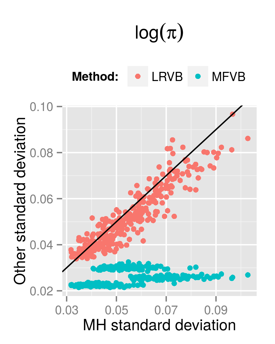
We wish to approximate the covariance matrix of the parameters $\log(\pi),\mu,\log(\tau)$ in the posterior distribution $p(\pi,\mu,\tau|x)$ from the preceding generative model. In our experiment, $K=3$ and $N=3000$ for each of 100 simulations. We compare three different approaches to compute the posterior covariance: a Metropolis-Hastings (MH) sampler, MFVB, and LRVB. The MH sampler draws independent proposals centered at the MAP estimate in order to avoid label-switching problems. The two VB solutions augment Eq. (8) with indicator variables, $z$ , which indicate which component each point was drawn from. We note that for each of the parameters $\log(\pi)$ , $\mu$ , and $\log(\tau)$ , both MH and MFVB produce point estimates close to the true values, so our key assumption in the LRVB derivations of Section 3 appears to hold. To compare the covariance matrices, we use MH as a ground truth; for the low-dimensional model we are using, it is reasonable to expect that MH should return a good approximation of the true posterior. We see in Fig. (1) that the LRVB estimates agree with the MH posterior variance while MFVB consistently underestimates the posterior variance.

Refer to caption — Figure 1: Comparison of estimates of the posterior standard deviation for each model parameter according to methods MH, MFVB, and LRVB and across 100 simulations.

4.2 Sensitivity analysis

Next consider a slight variation to the model of Section 4.1. We retain the distribution of $p(x|\pi,\mu,\tau)$ in Eq. (8) but now assume that the observed data $x^{*}$ are actually independent noisy versions of $x$ : $x_{n}^{*}\sim\mathcal{N}(x_{n},\sigma^{2}),$ for a deterministic constant $\sigma^{2}$ . We retain the prior on $\mu$ in Eq. (9), but fix $\pi$ and $\tau$ at their true values. In this new model, $x$ and $\mu$ are the unknown parameters. Using LRVB, we can estimate the posterior covariance between any $x_{n}$ and the mixture parameters $\mu$ . If we look at this covariance as $\sigma^{2}\rightarrow 0$ , we obtain a type of leverage score. That is, the limiting value of this covariance can be used to estimate the influence of observation $x_{n}$ on the mixture parameters in the spirit of classical linear model leverage scores from the statistics literature. LRVB leads to a straightforward analytic expression for these covariances, which can be found in Eq. (41) in Appendix C. ²² 2 Appendix C also includes a proof that this LRVB-limiting method reproduces classical leverage scores when applied to linear regression.

Note that these leverage scores are impossible to compute in naive MFVB, since they involve correlations between distinct mean field components, and difficult to compute using MH, since they require estimating a large number of very small covariances with a finite number of draws.

To evaluate these LRVB-derived leverage scores, we compare them to the effect of manually perturbing our data and re-fitting the model. Here, we choose $K=2$ components in the mixture model and $N=500$ . (The small $N$ is chosen to make the manual perturbation calculations more manageable.) The LRVB-derived leverage scores are plotted as a function of $x_{n}$ location on the lefthand side of Fig. (2). We can see from the comparison on the righthand side of Fig. (2) that the LRVB-derived leverage scores match well with the results of manual perturbation, which took over 30 times longer to compute.

As expected, the data points with the greatest effect on the location of a component are the ones most likely to be assigned to the component. Interestingly, though, data still retain leverage on a component even when they are assigned with certainty to the other component. Indeed, a data point assigned to one component with probability close to one will affect that component’s mean, which in turn affects the classification of other data points, which then affects the location of the other component. In this way, we see that LRVB is estimating covariances that are the results of complex chains of correlations.

Acknowledgments

The authors thank Michael I. Jordan for suggesting that we look at linear response theory and Alex Blocker for helpful comments. R. Giordano and T. Broderick were funded by Berkeley Fellowships.

References

[1] D. M. Blei, A. Y. Ng, and M. I. Jordan. Latent Dirichlet allocation. Journal of Machine Learning Research, 3:993–1022, 2003.
[2] D. M. Blei and M. I. Jordan. Variational inference for Dirichlet process mixtures. Bayesian Analysis, 1(1):121–143, 2006.
[3] M. D. Hoffman, D. M. Blei, C. Wang, and J. Paisley. Stochastic variational inference. Journal of Machine Learning Research, 14(1):1303–1347, 2013.
[4] B. Wang and M. Titterington. Inadequacy of interval estimates corresponding to variational Bayesian approximations. In Workshop on Artificial Intelligence and Statistics, pages 373–380, 2004.
[5] C. M. Bishop. Pattern Recognition and Machine Learning. Springer, New York, 2006. Chapter 10.
[6] H. Rue, S. Martino, and N. Chopin. Approximate Bayesian inference for latent Gaussian models by using integrated nested Laplace approximations. Journal of the Royal Statistical Society: Series B (statistical methodology), 71(2):319–392, 2009.
[7] R. E. Turner and M. Sahani. Two problems with variational expectation maximisation for time-series models. In D. Barber, A. T. Cemgil, and S. Chiappa, editors, Bayesian Time Series Models. 2011.
[8] H. J. Kappen and F. B. Rodriguez. Efficient learning in Boltzmann machines using linear response theory. Neural Computation, 10(5):1137–1156, 1998.
[9] M. Welling and Y. W. Teh. Linear response algorithms for approximate inference in graphical models. Neural Computation, 16(1):197–221, 2004.
[10] R. W. Keener. Theoretical Statistics. Springer, 2010.
[11] X. L. Meng and D. B. Rubin. Using EM to obtain asymptotic variance-covariance matrices: The SEM algorithm. Journal of the American Statistical Association, 86(416):899–909, 1991.

Appendix A Derivations

A.1 MFVB for conditional exponential families

Lemma A.1.

Suppose Eq. (2) holds across all $j$ ; that is,

p(\theta_{j}|\theta_{i:i\neq j},x)=\exp(\tilde{\eta}_{j}^{T}\theta_{j}-A_{j}(\tilde{\eta}_{j})).

Then, for the natural parameter $\tilde{\eta}_{j}$ , we have

\tilde{\eta}_{j}=\sum_{R\subseteq[J]\backslash\{j\}}G_{R}\prod_{r\in R}\theta_{r},

where $[J]:=\{1,\ldots,J\}$ and $G_{R}$ is constant in $\theta$ .

Proof.

We see that $\log p(\theta|x)=\log p(\theta_{j}|\theta_{i:i\neq j},x)+\log p(\theta_{i:i\neq j}|x)$ depends on $\theta_{j}$ only via the first term in the sum. So by Eq. (2), $\log p(\theta|x)$ is linear in $\theta_{j}$ , and we can write

\log p(\theta|x)=\sum_{R^{\prime}\subset[J]}G^{\prime}_{R^{\prime}}\prod_{r\in R^{\prime}}\theta_{r}+\mathrm{constant},

where $G^{\prime}_{R^{\prime}}$ and the final summand are constant in all of $\theta$ . The result follows by collecting those terms where $j\in R^{\prime}$ . ∎

A.2 Linear response

We here derive the three equalities in Eq. (6), which appear as three propositions below. In these propositions, we assume that $p(\theta|x)$ is in the exponential family as above. We will further assume that all natural parameters (for $p$ or variational approximations) are in the interior of the parameter space and that $t$ is sufficiently small. These assumptions will allow us to apply dominated convergence (cf. Section 2.3 of [10]).

Proposition A.2.

$\frac{d}{dt}\mathbb{E}_{p_{t}}\theta=\Sigma_{p_{t}}$ .

Proof.

	$\displaystyle\frac{d}{dt^{T}}\mathbb{E}_{p_{t}}\theta$	$\displaystyle=\frac{d}{dt^{T}}\int_{\theta}\theta e^{t^{T}\theta-c(t)}p(\theta\|x)d\theta\quad\textrm{by the definition of $p_{t}$ in Eq.~(\ref{eq:perturbed_dens})}$
		$\displaystyle=\int_{\theta}\theta\left[\frac{d}{dt^{T}}e^{t^{T}\theta-c(t)}\right]p(\theta\|x)d\theta\quad\textrm{by dominated convergence}$
		$\displaystyle=\int_{\theta}\theta\theta^{T}e^{t^{T}\theta-c(t)}p(\theta\|x)d\theta-\int_{\theta}\theta e^{t^{T}\theta-c(t)}p(\theta\|x)d\theta\cdot\frac{dc(t)}{dt^{T}}$
		$\displaystyle=\mathbb{E}_{p_{t}}\left[\theta\theta^{T}\right]-\mathbb{E}_{p_{t}}\left[\theta\right]\mathbb{E}_{p_{t}}\left[\theta\right]^{T}=\Sigma_{p_{t}}$

∎

To approximate $\frac{dm_{t}}{dt^{T}}$ , we assume not only that $m_{t}\approx\mathbb{E}_{p_{t}}\theta$ for any particular $t$ but further that $m_{t}$ tracks the true mean $\mathbb{E}_{p_{t}}\theta$ as $t$ varies. In this case, by Proposition A.2, we have

\frac{dm_{t}}{dt^{T}}\approx\frac{d}{dt^{T}}\mathbb{E}_{p_{t}}\theta=\Sigma_{p_{t}},

the first (approximate) equality in Eq. (6).

To derive the final two equalities in Eq. (6), we make use of the following lemma.

Lemma A.3.

$M_{t,j}$ depends on $t$ only via $\eta_{t,j}$ , the natural parameter of the $q_{t,j}^{*}$ distribution. And $\frac{dM_{t,j}}{d\eta_{t,j}^{T}}=\Sigma_{q_{t,j}^{*}}$ .

Proof.

The first part of the lemma follows from writing the definition of $M_{t,j}$ :

M_{t,j}=\mathbb{E}_{q_{t,j}^{*}}\theta_{j}=\int_{\theta_{j}}\theta_{j}\exp\left(\eta_{t,j}^{T}\theta_{j}-A_{j}\left(\eta_{t,j}\right)\right)d\theta_{j}.

For the second part,

	$\displaystyle\frac{dM_{t,j}}{d\eta_{t,j}^{T}}$	$\displaystyle=\int_{\theta_{j}}\frac{d}{d\eta_{t,j}^{T}}\theta_{j}\exp\left(\eta_{t,j}^{T}\theta_{j}-A_{j}\left(\eta_{t,j}\right)\right)d\theta_{j}\quad\textrm{by dominated convergence}$
		$\displaystyle=\int_{\theta_{j}}\theta_{j}\left[\theta_{j}^{T}-\mathbb{E}_{q_{t,j}^{*}}\theta_{j}^{T}\right]\exp\left(\eta_{t,j}^{T}\theta_{j}-A_{j}\left(\eta_{t,j}\right)\right)d\theta_{j}$
		$\displaystyle=\Sigma_{q_{t,j}^{*}}$

∎

Proposition A.4.

$\frac{\partial M_{t}}{\partial t^{T}}=\Sigma_{q_{t}^{*}}.$

Proof.

By Lemma A.3, we have for any indices $i$ and $j$ in $[J]$ that

\frac{\partial M_{t,j}}{\partial t_{i}^{T}}=\frac{dM_{t,j}}{d\eta_{t,j}^{T}}\frac{\partial\eta_{t,j}}{\partial t_{i}^{T}},

(10)

where the first factor is also given by Lemma A.3. It remains to find the second factor, $\frac{\partial\eta_{t,j}}{\partial t_{i}^{T}}$ . By the discussion after Eq. (2) and the construction of $p_{t}$ , the natural parameter $\tilde{\eta}_{t,j}$ of $p_{t}\left(\theta_{j}|\theta_{i:i\neq j},x\right)$ satisfies

\tilde{\eta}_{t,j}=\sum_{R\subseteq[J]/\{j\}}G_{R}\prod_{r\in R}\theta_{r}+t_{j}.

So, as in the derivation of Eq. (3), the natural parameter $\eta_{t,j}$ of $q_{j}^{*}(\theta_{j})$ satisfies

\eta_{t,j}=\sum_{R\subseteq[J]/\{j\}}G_{R}\prod_{r\in R}m_{t,r}+t_{j}

(11)

for $m_{t,r}:=\mathbb{E}_{q^{*}_{t,r}}\theta_{r}$ .

Let $d_{j}$ be the dimension of $\theta_{j}$ and hence the dimension of $\eta_{t,j}$ and $t_{j}$ . Hence,

\frac{\partial\eta_{t,j}}{\partial t_{i}^{T}}=\left\{\begin{array}[]{ll}I_{d_{j}}&j=i\\ 0_{d_{j},d_{i}}&\mathrm{else}\end{array}\right.,

where $I_{a}$ is the identity matrix of dimension $a$ , and $0_{a,b}$ is the all zeros matrix of dimension $a\times b$ .

Finally, by Eq. (10), Lemma A.3, and the expression for $\frac{\partial\eta_{t,j}}{\partial t_{i}^{T}}$ just obtained, we have

\frac{\partial M_{t}}{\partial t^{T}}=\Sigma_{q_{t}^{*}}I_{D}=\Sigma_{q_{t}^{*}}.

∎

Proposition A.5.

$\frac{dM_{t}}{dm_{t}^{T}}=\Sigma_{q_{t}^{*}}\frac{\partial\eta_{t}}{\partial m_{t}^{T}}.$

Proof.

By Lemma A.3 and analogous to Eq. (10), we have

\frac{\partial M_{t,j}}{\partial m_{t,i}^{T}}=\frac{dM_{t,j}}{d\eta_{t,j}^{T}}\frac{\partial\eta_{t,j}}{\partial m_{t,i}^{T}}.

(12)

The result follows immediately from Lemma A.3. ∎

Appendix B Multivariate normal

For any target distribution $p(\theta|x)$ , it is well-known that MFVB cannot be used to estimate the covariances between the components of $\theta$ . In particular, if $q^{*}$ is the estimate of $p(\theta|x)$ returned by MFVB, $q^{*}$ will have a block-diagonal covariance matrix—no matter the form of the covariance of $p(\theta|x)$ . By contrast, the next result shows that the LRVB covariance estimate is exactly correct in the case where the target distribution, $p(\theta|x)$ , is (multivariate) normal.

In order to prove this result, we will rely on the following lemma.

Lemma B.1.

Consider a target posterior distribution characterized by $p(\theta|x)=\mathcal{N}(\theta|\mu,\Sigma)$ , where $\mu$ and $\Sigma$ may depend on $x$ , and $\Sigma$ is invertible. Let $\theta=(\theta_{1},\ldots,\theta_{J})$ , and consider a MFVB approximation to $p(\theta|x)$ that factorizes as $q(\theta)=\prod_{j}q(\theta_{j})$ . Then the variational posterior means are the true posterior means; i.e. $m_{j}=\mu_{j}$ for all $j$ between $1$ and $J$ .

Proof.

The derivation of MFVB for the multivariate normal can be found in Section 10.1.2 of [5]; we highlight some key results here. Let $\Lambda=\Sigma^{-1}$ . Let the $j$ index on a row or column correspond to $\theta_{j}$ , and let the $-j$ index correspond to $\{\theta_{i}:i\neq j\}$ . E.g., for $j=1$ ,

\Lambda=\left[\begin{array}[]{ll}\Lambda_{11}&\Lambda_{1,-1}\\ \Lambda_{-1,1}&\Lambda_{-1,-1}\end{array}\right].

By the assumption that $p(\theta|x)=\mathcal{N}(\theta|\mu,\Sigma)$ , we have

\log p(\theta_{j}|\theta_{i:i\neq j},x)=-\frac{1}{2}(\theta_{j}-\mu_{j})^{T}\Lambda_{jj}(\theta_{j}-\mu_{j})+(\theta_{j}-\mu_{j})^{T}\Lambda_{j,-j}(\theta_{-j}-\mu_{-j})+\mathrm{constant},

(13)

where the final term is constant in $\theta_{j}$ . It follows that

	$\displaystyle\log q^{*}_{j}(\theta_{j})$	$\displaystyle=\mathbb{E}_{q^{*}_{i}:i\neq j}\log p(\theta,x)+\mathrm{constant}$
		$\displaystyle=-\frac{1}{2}\theta_{j}^{T}\Lambda_{jj}\theta_{j}+\theta_{j}\mu_{j}\Lambda_{jj}-\theta_{j}\Lambda_{j,-j}(\mathbb{E}_{q^{*}}\theta_{-j}-\mu_{-j}).$

q^{*}_{j}(\theta_{j})=\mathcal{N}(\theta_{j}|m_{j},\Lambda_{jj}^{-1}),

with mean parameters

m_{j}=\mathbb{E}_{q^{*}_{j}}\theta_{j}=\mu_{j}-\Lambda_{jj}^{-1}\Lambda_{j,-j}(m_{-j}-\mu_{-j})

(14)

as well as an equation for $\mathbb{E}_{q^{*}}\theta^{T}\theta$ .

Note that $\Lambda_{jj}$ must be invertible, for if it were not, $\Sigma$ would not be invertible.

The solution $m=\mu$ is a unique stable point for Eq. (14), since the fixed point equations for each $j$ can be stacked and rearranged to give

$\displaystyle m-\mu$	$\displaystyle=$	$\displaystyle-\left[\begin{array}[]{ccccc}0&\Lambda_{11}^{-1}\Lambda_{12}&\cdots&\Lambda_{11}^{-1}\Lambda_{1\left(J-1\right)}&\Lambda_{11}^{-1}\Lambda_{1J}\\ \vdots&&\ddots&&\vdots\\ \Lambda_{JJ}^{-1}\Lambda_{J1}&\Lambda_{JJ}^{-1}\Lambda_{J2}&\cdots&\Lambda_{JJ}^{-1}\Lambda_{J\left(J-1\right)}&0\end{array}\right]\left(m-\mu\right)$
	$\displaystyle=$	$\displaystyle-\left[\begin{array}[]{ccccc}\Lambda_{11}^{-1}&\cdots&0&\cdots&0\\ \vdots&\ddots&&&\vdots\\ 0&&\ddots&&0\\ \vdots&&&\ddots&\vdots\\ 0&\cdots&0&\cdots&\Lambda_{JJ}^{-1}\end{array}\right]\left[\begin{array}[]{ccccc}0&\Lambda_{12}&\cdots&\Lambda_{1\left(J-1\right)}&\Lambda_{1J}\\ \vdots&&\ddots&&\vdots\\ \Lambda_{J1}&\Lambda_{J2}&\cdots&\Lambda_{J\left(J-1\right)}&0\end{array}\right]\left(m-\mu\right)\Leftrightarrow$
$\displaystyle 0$	$\displaystyle=$	$\displaystyle\left[\begin{array}[]{ccccc}\Lambda_{11}&\cdots&0&\cdots&0\\ \vdots&\ddots&&&\vdots\\ 0&&\ddots&&0\\ \vdots&&&\ddots&\vdots\\ 0&\cdots&0&\cdots&\Lambda_{JJ}\end{array}\right]\left(m-\mu\right)+$
		$\displaystyle\left[\begin{array}[]{ccccc}0&\Lambda_{12}&\cdots&\Lambda_{1\left(J-1\right)}&\Lambda_{1J}\\ \vdots&&\ddots&&\vdots\\ \Lambda_{J1}&\Lambda_{J2}&\cdots&\Lambda_{J\left(J-1\right)}&0\end{array}\right]\left(m-\mu\right)\Leftrightarrow$
$\displaystyle 0$	$\displaystyle=$	$\displaystyle\Lambda\left(m-\mu\right)\Leftrightarrow$
$\displaystyle m$	$\displaystyle=$	$\displaystyle\mu.$

The last step follows from the assumption that $\Sigma$ (and hence $\Lambda$ ) is invertible. It follows that $\mu$ is the unique stable point of Eq. (14).

∎

Proposition B.2.

Assume we are in the setting of Lemma B.1, where additionally $\mu$ and $\Sigma$ are on the interior of the feasible parameter space. Then the LRVB covariance estimate exactly captures the true covariance, $\hat{\Sigma}=\Sigma$ .

Proof.

Consider the perturbation for LRVB defined in Eq. (4). By perturbing the log likelihood, we change both the true means $\mu_{t}$ and the variational solutions, $m_{t}$ . The result is a valid density function since the original $\mu$ and $\Sigma$ are on the interior of the parameter space. By Lemma B.1, the MFVB solutions are exactly the true means, so $m_{t,j}=\mu_{t,j}$ , and the derivatives are the same as well. This means that the first term in Eq. (7) is not approximate, i.e.

\frac{dm_{t}}{dt^{T}}=\frac{d}{dt^{T}}\mathbb{E}_{p_{t}}\theta=\Sigma_{p_{t}},

It follows from the arguments in Appendix B that the LRVB covariance matrix is exact, and $\hat{\Sigma}=\Sigma$ .

∎

One final result about the multivariate normal will simplify some of the leverage score calculations to follow. The variational distribution in Eq. (13) has both linear and quadratic sufficient statistics for $\theta_{j}$ . That is, the full set of variational parameters are $\tilde{\theta}_{j}:=\left(\theta_{j}^{T},s_{j}^{T}\right)^{T}$ , where $s_{j}=\textrm{Vec}\left(\theta_{j}\otimes\theta_{j}\right)$ . (The Vec operator stacks a matrix columnwise into a vector, and $\otimes$ denotes the Kronecker product.)

Stictly speaking, Eq. (7) requires calculating derivatives for all the sufficient statistics, not just the statistics that we are interested in. However, when calculating the LRVB covariance for the mean of a normal distribution, we can effectively ignore the $s$ terms and apply Eq. (7) only to the $\theta$ terms.

Lemma B.3.

The LRVB covariance matrix for the mean of a multivariate normal distribution does not depend on the sensitivities to the quadratic sufficient statistics. Specifically,

\hat{\Sigma}_{\theta}=\left(I-\frac{\partial M_{\theta}}{\partial m_{\theta}}\right)^{-1}\Sigma_{q^{*},\theta}

(19)

Proof.

We will evaluate the terms in Eq. (7) for the full parameter vector $\tilde{\theta}$ , and show that the submatrix of $\hat{\Sigma}$ corresponding to $\theta$ is given by Eq. (19).

Partition the matrices $H$ and $\Sigma_{q^{*}}$ from Eq. (7) into blocks for $\theta$ and $s$ . We will use $V_{\theta}$ and $V_{s}$ to denote the variational variance of $\theta$ and $s$ , and $V_{\theta s}$ to denote the variational covariance between $\theta$ and $s$ . All the $V$ terms are given by standard properties of the multivariate normal distribution.

	$\displaystyle H$	$\displaystyle=$	$\displaystyle\left(\begin{array}[]{cc}\frac{\partial\eta_{\theta}}{\partial m_{\theta}}&\frac{\partial\eta_{\theta}}{\partial m_{s}}\\ \frac{\partial\eta_{s}}{\partial m_{\theta}}&0\end{array}\right)=\left(\begin{array}[]{cc}\frac{\partial\eta_{\theta}}{\partial m_{\theta}}&0\\ 0&0\end{array}\right)$
	$\displaystyle\Sigma_{q^{*}}$	$\displaystyle=$	$\displaystyle\left(\begin{array}[]{cc}V_{\theta}&V_{\theta s}\\ V_{\theta s}^{T}&V_{s}\end{array}\right)$

In the formula for $H$ , we have used the observation from Eq. (13) that the terms of $s$ never co-occur with any other terms of $\tilde{\theta}$ , so that $\frac{\partial\eta_{s}}{\partial m_{\theta}^{T}}=\frac{\partial\eta_{\theta}^{T}}{\partial m_{s}}=0$ .

First, we calculate:

	$\displaystyle\left(I-\Sigma_{q^{*}}H\right)$	$\displaystyle=$	$\displaystyle I-\left(\begin{array}[]{cc}V_{\theta}&V_{\theta s}\\ V_{\theta s}^{T}&V_{s}\end{array}\right)\left(\begin{array}[]{cc}\frac{\partial\eta_{\theta}}{\partial m_{\theta}}&0\\ 0&0\end{array}\right)$
		$\displaystyle=$	$\displaystyle\left(\begin{array}[]{cc}I-V_{\theta}\frac{\partial\eta_{\theta}}{\partial m_{\theta}}&0\\ -V_{\theta s}^{T}\frac{\partial\eta_{\theta}}{\partial m_{\theta}}&I\end{array}\right)$

Using the Schur inverse and the fact that the upper right hand corner is the $0$ matrix, we can write

\displaystyle\left(I-\Sigma_{q^{*}}H\right)^{-1}

\displaystyle=

\displaystyle\left(\begin{array}[]{cc}\left(I-V_{\theta}\frac{\partial\eta_{\theta}}{\partial m_{\theta}}\right)^{-1}&0\\ Q_{\theta s}&Q_{ss}\end{array}\right),

where $Q_{\theta s}$ and $Q_{ss}$ are simply placeholders for the rest of the inverse. Multiplying by $\Sigma_{q^{*}}$ gives that the $\theta$ -sized upper-left corner of $\hat{\Sigma}$ is

\displaystyle\hat{\Sigma}_{\theta\theta}

\displaystyle=

\displaystyle\left(I-V_{\theta}\frac{\partial\eta_{\theta}}{\partial m_{\theta}}\right)^{-1}V_{\theta}

This is the same as Eq. (19) and identical to what we would have gotten by applying Eq. (7) to $\theta$ alone, ignoring the $s$ dependence.

∎

B.1 Comparison with supplemented expectation-maximization

This result about the multivariate normal distribution draws a connection between LRVB corrections and the “supplemented expectation-maximization” (SEM) method of [11]. SEM is an asymptotically exact covariance correction for the EM algorithm that transforms the full-data Fisher information matrix into the observed-data Fisher information matrix using a correction that is formally similar to Eq. (7). In this section, we argue that this similarity is not a coincidence; in fact the SEM correction is an asymptotic version of LRVB with two variational blocks, one for the missing data and one for the unknown parameters.

Although LRVB as described here requires a prior (unlike SEM, which supplements the MLE), the two covariance corrections coincide when the full information likelihood is approximately log quadratic and proportional to the posterior, $p(\theta|x)$ . This might be expected to occur when we have a large number of independent data points informing each parameter—i.e., when a central limit theorem applies and the priors do not affect the posterior. In the full information likelihood, some terms may be viewed as missing data, whereas in the Bayesian model the same terms may be viewed as latent parameters, but this does not prevent us from formally comparing the two methods.

We can draw a term-by-term analogy with the equations in [11]. We denote variables from the SEM paper with a superscript “ $SEM$ ” to avoid confusion. MFVB does not differentiate between missing data and parameters to be estimated, so our $\theta$ corresponds to $(\theta^{SEM},Y_{mis}^{SEM})$ in [11]. SEM is an asymptotic theory, so we may assume that $(\theta^{SEM},Y_{mis}^{SEM})$ have a multivariate normal distribution, and that we are interested in the mean and covariance of $\theta^{SEM}$ .

In the E-step of [11], we replace $Y_{mis}^{SEM}$ with its conditional expectation given the data and other $\theta^{SEM}$ . This corresponds precisely to Eq. (14), taking $\theta_{j}=Y_{mis}^{SEM}$ . In the M-step, we find the maximum of the log likelihood with respect to $\theta^{SEM}$ , keeping $Y_{mis}^{SEM}$ fixed at its expectation. Since the mode of a multivariate normal distribution is also its mean, this, too, corresponds to Eq. (14), now taking $\theta_{j}=\theta^{SEM}$ .

It follows that the MFVB and EM fixed point equations are the same; i.e., our $M$ is the same as their $M^{SEM}$ , and our $\partial M/\partial m$ of Eq. (6) corresponds to the transpose of their $DM^{SEM}$ , defined in Eq. (2.2.1) of [11]. Since the “complete information” corresponds to the variance of $\theta^{SEM}$ with fixed values for $Y_{OBS}^{SEM}$ , this is the same as our $\Sigma_{q^{*},11}$ , the variational covariance, whose inverse is $I_{oc}^{-1}$ . Taken all together, this means that equation (2.4.6) of [11] can be re-written as our Eq. (7).

	$\displaystyle V^{SEM}=$	$\displaystyle I_{oc}^{-1}\left(I-DM^{SEM}\right)^{-1}\Rightarrow$
	$\displaystyle\Sigma=$	$\displaystyle\Sigma_{q^{}}\left(I-\left(\frac{\partial M}{\partial m^{T}}\right)^{T}\right)^{-1}=\left(I-\frac{\partial M}{\partial m^{T}}\right)^{-1}\Sigma_{q^{}}$

Appendix C Leverage scores

In a linear model $y_{i}=\beta^{T}x_{i}+\epsilon$ , leverage score estimates how much influence each observation $x_{i}$ has on its fitted value, $\hat{y_{i}}=\hat{\beta}x_{i}$ , through its influence on $\hat{\beta}$ . In an analogous Bayesian way, we can use LRVB to estimate the correlation between infinitesimal noise in our observed data and our posterior estimates of $\theta=\left(\mu,\sigma,p\right)$ in the model of Section 4 .

In this appendix, we first show that covariance-based “leverage scores” described in Section 4.2 are the same as classical leverage scores for linear models. Then, we derive the leverage scores for the means of a normal mixture model.

C.1 Linear model leverage scores

Let us define a classical linear regression with known variance as

	$\displaystyle y_{i}$	$\displaystyle\sim$	$\displaystyle\mathcal{N}\left(\beta^{T}x_{i},\sigma^{2}\right)$
	$\displaystyle\log p\left(Y\|\beta\right)$	$\displaystyle=$	$\displaystyle-\frac{1}{2\sigma^{2}}\beta^{T}X^{T}X\beta+\frac{1}{\sigma^{2}}Y^{T}X\beta+\mathrm{constant}.$

Here, in order to take advantage of familiar matrix formulas for linear regression, we will use capital letters to denote vectors and matrices in this section. That is, $Y$ is the vector of scalars $y_{i}$ , $X$ is the matrix formed by stacking the observations $x_{i}^{T}$ . To recover leverage scores, suppose that instead of $y_{i}$ , we observe normal random variables $y_{i}^{*}$ , where:

	$\displaystyle E(y_{i}^{*}\|y_{i})$	$\displaystyle=$	$\displaystyle y_{i}$
	$\displaystyle Var(y_{i}^{*}\|y_{i})$	$\displaystyle=$	$\displaystyle\epsilon.$

The variables $y_{i}$ and $y_{i}^{*}$ are analogous to the variables $x_{i}$ and $x_{i}^{*}$ of Section 4.2, respectively. We will then use MFVB to fit this model where the parameters to be estimated are $\theta=(Y^{T},\beta^{T})^{T}$ and we have a uniform improper prior on $\beta$ . Since the posterior is multivariate normal, in this case the LRVB covariance matrices for $\theta$ will be exact in light of Appendix B.

The sufficient statistics for $Y$ include quadratic terms, $y_{i}^{2}$ , that are correlated with the linear sufficient statistics. Ordinarily, one must also include derivatives with respect to these quadratic sufficient statistics when applying Eq. (7) (as is done in Section C.2). However, since the posterior is multivariate normal, we can apply Lemma B.3 and only consider the sensitivity to $Y$ .

The terms in Eq. (7) are given by:

$\displaystyle\Sigma_{q^{*}_{Y}}$	$\displaystyle=$	$\displaystyle\textrm{Var}(Y\|\beta,Y^{*})=\epsilon I_{Y}$
$\displaystyle\Sigma_{q^{*}_{\beta}}$	$\displaystyle=$	$\displaystyle\textrm{Var}(\beta\|Y,Y^{*})=\left(X^{T}X\right)^{-1}\sigma^{2}$
$\displaystyle\frac{\partial\eta_{\beta}}{\partial m_{Y}^{T}}$	$\displaystyle=$	$\displaystyle\frac{1}{\sigma^{2}}X^{T}$
$\displaystyle\frac{\partial\eta_{Y}}{\partial m_{\beta}^{T}}$	$\displaystyle=$	$\displaystyle\frac{1}{\sigma^{2}}X\Rightarrow$
$\displaystyle I-\Sigma_{q^{*}}H$	$\displaystyle=$	$\displaystyle\left(\begin{array}[]{cc}I_{\beta}&-\sigma^{2}\left(X^{T}X\right)^{-1}X^{T}\\ -\frac{\epsilon}{\sigma^{2}}X&I_{Y}\end{array}\right).$

The upper-left ( $\beta$ ) component of $(I-\Sigma_{q^{*}}H)^{-1}$ can be calculated with the Schur complement:

$\displaystyle\left(I-\Sigma_{q^{*}}H\right)_{\beta\beta}^{-1}$	$\displaystyle=$	$\displaystyle\left(I_{\beta}-\frac{\epsilon}{\sigma^{2}}\left(X^{T}X\right)^{-1}X^{T}X\right)^{-1}$
	$\displaystyle=$	$\displaystyle\left(1-\frac{\epsilon}{\sigma^{2}}\right)^{-1}I_{\beta}$
	$\displaystyle\equiv$	$\displaystyle\alpha I_{\beta},$

where we have defined $\alpha=\sigma^{2}\left(\sigma^{2}-\epsilon\right)^{-1}$ . Note that $\lim_{\epsilon\rightarrow 0}\alpha=1$ . This gives the rest of the inverse and the covariance between $Y$ and $\beta$ :

$\displaystyle\left(I-\Sigma_{q^{*}}H\right)^{-1}$	$\displaystyle=$	$\displaystyle\left(\begin{array}[]{cc}\alpha I_{\beta}&\alpha\left(X^{T}X\right)^{-1}X^{T}\\ \alpha\frac{\epsilon}{\sigma^{2}}X&\left(I_{Y}-\frac{\epsilon}{\sigma^{2}}P_{X}\right)^{-1}\end{array}\right)$
$\displaystyle\Sigma_{p}$	$\displaystyle=$	$\displaystyle\left(\begin{array}[]{cc}\alpha I_{\beta}&\alpha\left(X^{T}X\right)^{-1}X^{T}\\ \alpha\frac{\epsilon}{\sigma^{2}}X&\left(I_{Y}-\frac{\epsilon}{\sigma^{2}}P_{X}\right)^{-1}\end{array}\right)\left(\begin{array}[]{cc}\sigma^{2}\left(X^{T}X\right)^{-1}&0\\ 0&\epsilon I_{Y}\end{array}\right)$
	$\displaystyle=$	$\displaystyle\left(\begin{array}[]{cc}\alpha\sigma^{2}\left(X^{T}X\right)^{-1}&\epsilon\alpha\left(X^{T}X\right)^{-1}X^{T}\\ \epsilon\alpha X\left(X^{T}X\right)^{-1}&\epsilon\left(I_{Y}-\frac{\epsilon}{\sigma^{2}}P_{X}\right)^{-1}\end{array}\right),$

where $P_{X}=X\left(X^{T}X\right)^{-1}X^{T}$ is the projection matrix onto $X$ . This says that

$\displaystyle\textrm{Cov}(\beta,Y\|Y^{*})$	$\displaystyle=$	$\displaystyle\epsilon\alpha\left(X^{T}X\right)^{-1}X^{T}\Rightarrow$
$\displaystyle\textrm{Cov}(\hat{Y},Y\|Y^{*})$	$\displaystyle=$	$\displaystyle Cov(X\beta,Y)=XCov(\beta,Y)$
	$\displaystyle=$	$\displaystyle\epsilon\alpha P_{X}.$

Since $\epsilon\rightarrow 0\Rightarrow\alpha\rightarrow 1$ , the covariance between $\hat{y}_{i}$ and $z_{i}$ is proportional to the diagonal of $P_{X}$ , which is exactly the classical leverage score.

C.2 Normal mixture leverage scores

We now consider leverage scores in the setting of Section 4.2, The new posterior with perturbed $x$ observations is the original posterior plus a term for $x^{*}$ :

	$\displaystyle\log p\left(\mu,\sigma,a,z,x\|x^{*}\right)$	$\displaystyle=$	$\displaystyle\log p\left(\mu,\sigma,a,z\|x\right)+\log p\left(x\|x^{*}\right)+\mathrm{constant}$
		$\displaystyle=$	$\displaystyle\log p\left(\mu,\sigma,a,z\|x\right)-\frac{1}{2}\sigma_{x}^{-2}\sum_{i}\left(x_{i}-x_{i}^{*}\right)^{2}+\mathrm{constant}.$

We can imagine estimating each of the unobserved $x_{i}$ its own varational distribution with sufficient statistics $x_{i}$ and $x_{i}^{2}$ , though since we are adding infinitesimal noise, it is not necessary to actually re-fit the model. Infinitesimal noise in $x$ will not change the point estimates of $\theta$ , and since $\sigma_{x}\approx 0$ , only the $x_{i}^{*}$ terms matter for the variational posterior of $x_{i}$ . Using standard properties of the normal distribution and the fact that $\sigma_{x}\approx 0$ , the variational expectations of the sufficient statistics are then given by:

$\displaystyle E_{q*}\left(x_{i}\right)$	$\displaystyle=$	$\displaystyle x_{i}^{*}$	(29)
$\displaystyle E_{q*}\left(x_{i}^{2}\right)$	$\displaystyle=$	$\displaystyle\sigma_{x}^{2}+x_{i}^{*2}$	(30)
$\displaystyle\textrm{Var}_{q*}\left(x_{i}\right)$	$\displaystyle=$	$\displaystyle\sigma_{x}^{2}$	(31)
$\displaystyle\textrm{Var}_{q*}\left(x_{i}^{2}\right)$	$\displaystyle=$	$\displaystyle 4x_{i}^{2}\sigma_{x}^{2}+2\sigma_{x}^{4}\approx 4x_{i}^{2}\sigma_{x}^{2}$	(32)
$\displaystyle\textrm{Cov}_{q*}\left(x_{i}^{2}\right)$	$\displaystyle=$	$\displaystyle x_{i}^{*}\sigma_{x}^{2}.$	(33)

It will be notationally convenient to stack the sufficient statistics $x_{i}$ and $x_{i}^{2}$ in a single vector, simply called $x$ . $E_{q*}\left(x\right)$ and $\textrm{Var}_{q*}\left(x\right)$ , the variational mean and covarivance of $x$ , can be read off Eq. (29). We will also define $V_{x}$ by:

\displaystyle\textrm{Var}_{q*}\left(x\right)

\displaystyle:=

\displaystyle\sigma_{x}^{2}V_{x}.

To get the LRVB covariance, we need only to calculate the quantities in equation 7. In particular, we are interested in the sub-matrix $\hat{\Sigma}_{\theta x}$ , the estimated covariance between $\theta$ and $x$ . Although we will derive the covariance between $\theta$ and all of $x$ , we can keep in mind that the leverage scores are actually the submatrix of this covariance that corresponds to the $x_{i}$ terms, not the $x_{i}^{2}$ terms.

To aid our computation, we will use Schur compliments and the fact that $\sigma_{x}^{2}\approx 0$ . In order to make the notation tidier, we will use some shorthand notation relative to the main body of the text:

	$\displaystyle V$	$\displaystyle:=$	$\displaystyle\Sigma_{q*}$
	$\displaystyle R$	$\displaystyle:=$	$\displaystyle\Sigma_{q*}H.$

We partition each matrix into $\theta$ , $x$ , and $z$ blocks:

$\displaystyle\hat{\Sigma}$	$\displaystyle=$	$\displaystyle\left(\begin{array}[]{ccc}\hat{\Sigma}_{\theta\theta}&\hat{\Sigma}_{\theta X}&\hat{\Sigma}_{\theta Z}\\ \hat{\Sigma}_{X\theta}&\hat{\Sigma}_{XX}&\hat{\Sigma}_{XZ}\\ \hat{\Sigma}_{Z\theta}&\hat{\Sigma}_{ZX}&\hat{\Sigma}_{ZZ}\end{array}\right)$
$\displaystyle R$	$\displaystyle=$	$\displaystyle\left(\begin{array}[]{ccc}R_{\theta}&R_{\theta X}&R_{\theta Z}\\ R_{X\theta}&0&R_{XZ}\\ R_{Z\theta}&R_{ZX}&0\end{array}\right)$
$\displaystyle V$	$\displaystyle=$	$\displaystyle\left(\begin{array}[]{ccc}V_{\theta}&0&0\\ 0&\sigma_{x}^{2}V_{x}&0\\ 0&0&V_{Z}\end{array}\right).$

We are interested in using equation 7, i.e. $\Sigma=\left(I-R\right)^{-1}V$ , to find the sub-matrix in $\Sigma_{x\theta}$ . (We could just as well find $\Sigma_{\theta x}$ .) First, note that one can eliminate $z$ immediately with a Schur complement. In general, if the matrices partition into two groups $A$ and $B$ , then

\displaystyle\hat{\Sigma}_{A}

\displaystyle=

\displaystyle\left[I-R_{AA}-R_{AB}\left(I-R_{BB}\right)^{-1}R_{BA}\right]^{-1}V_{A}.

(37)

In this case, let $B$ refer to the $z$ variables and $a$ to everything else. Noting that $R_{ZZ}=0$ and applying formula 37 gives

$\displaystyle\left(\begin{array}[]{cc}\hat{\Sigma}_{\theta\theta}&\hat{\Sigma}_{\theta X}\\ \hat{\Sigma}_{X\theta}&\hat{\Sigma}_{XX}\end{array}\right)$	$\displaystyle=$	$\displaystyle\left[\left(\begin{array}[]{cc}I_{\theta}&0\\ 0&I_{X}\end{array}\right)-\left(\begin{array}[]{cc}R_{\theta}&R_{\theta X}\\ R_{X\theta}&0\end{array}\right)-\left(\begin{array}[]{c}R_{\theta Z}\\ R_{XZ}\end{array}\right)\left(\begin{array}[]{cc}R_{Z\theta}&R_{ZX}\end{array}\right)\right]^{-1}\left(\begin{array}[]{cc}V_{\theta}&0\\ 0&\sigma_{x}^{2}V_{x}\end{array}\right)$
	$\displaystyle=$	$\displaystyle\left[\left(\begin{array}[]{cc}I_{\theta}-R_{\theta}&-R_{\theta X}\\ -R_{X\theta}&I_{X}\end{array}\right)-\left(\begin{array}[]{cc}R_{\theta Z}R_{Z\theta}&R_{\theta Z}R_{ZX}\\ R_{XZ}R_{Z\theta}&R_{XZ}R_{ZX}\end{array}\right)\right]^{-1}\left(\begin{array}[]{cc}V_{\theta}&0\\ 0&\sigma_{x}^{2}V_{x}\end{array}\right)$
	$\displaystyle=$	$\displaystyle\left(\begin{array}[]{cc}\left(I_{\theta}-R_{\theta}-R_{\theta Z}R_{Z\theta}\right)&\left(-R_{\theta X}-R_{\theta Z}R_{ZX}\right)\\ \left(-R_{X\theta}-R_{XZ}R_{Z\theta}\right)&\left(I_{X}-R_{XZ}R_{ZX}\right)\end{array}\right)^{-1}\left(\begin{array}[]{cc}V_{\theta}&0\\ 0&\sigma_{x}^{2}V_{x}\end{array}\right).$

It will be enough to get the first row, $\left(\hat{\Sigma}_{\theta\theta},\hat{\Sigma}_{\theta X}\right)$ , and for that we can use the Schur inverse.

$\displaystyle BD^{-1}C$	$\displaystyle=$	$\displaystyle\left(R_{\theta X}+R_{\theta Z}R_{ZX}\right)\left(I_{X}-R_{XZ}R_{ZX}\right)^{-1}\left(R_{X\theta}+R_{XZ}R_{Z\theta}\right)$
$\displaystyle A-BD^{-1}C$	$\displaystyle=$	$\displaystyle I_{\theta}-R_{\theta}-R_{\theta Z}R_{Z\theta}-\left(R_{\theta X}+R_{\theta Z}R_{ZX}\right)\left(I_{X}-R_{XZ}R_{ZX}\right)^{-1}\left(R_{X\theta}+R_{XZ}R_{Z\theta}\right)$
$\displaystyle BD^{-1}$	$\displaystyle=$	$\displaystyle-\left(R_{\theta X}+R_{\theta Z}R_{ZX}\right)\left(I_{X}-R_{XZ}R_{ZX}\right)^{-1}.$

Given these quantities, since the $V$ matrix is block diagonal,

\displaystyle\hat{\Sigma}_{\theta X}

\displaystyle=

\displaystyle-\left(A-BD^{-1}C\right)^{-1}BD^{-1}V_{x}\sigma_{x}^{2}.

It will be helpful to simplify this by taking $\sigma_{x}^{2}\rightarrow 0$ . To aid in this, write:

$\displaystyle R_{XZ}$	$\displaystyle=$	$\displaystyle\sigma_{x}^{2}Q_{XZ}$
$\displaystyle R_{X\theta}$	$\displaystyle=$	$\displaystyle\sigma_{x}^{2}Q_{X\theta}$
$\displaystyle D^{-1}=\left(I_{X}-R_{XZ}R_{ZX}\right)^{-1}$	$\displaystyle=$	$\displaystyle\left(I_{X}-\sigma_{x}^{2}Q_{XZ}R_{ZX}\right)^{-1}$
	$\displaystyle\approx$	$\displaystyle I_{X}+\sigma_{x}^{2}Q_{XZ}R_{ZX}.$

Then:

$\displaystyle A-BD^{-1}C$	$\displaystyle\approx$	$\displaystyle I_{\theta}-R_{\theta}-R_{\theta Z}R_{Z\theta}-\sigma_{x}^{2}\left(R_{\theta X}+R_{\theta Z}R_{ZX}\right)\left(I_{X}+\sigma_{x}^{2}Q_{XZ}R_{ZX}\right)\left(Q_{X\theta}+Q_{XZ}R_{Z\theta}\right)$
	$\displaystyle\approx$	$\displaystyle I_{\theta}-R_{\theta}-R_{\theta Z}R_{Z\theta}-\sigma_{x}^{2}\left(R_{\theta X}+R_{\theta Z}R_{ZX}\right)\left(Q_{X\theta}+Q_{XZ}R_{Z\theta}\right)$
$\displaystyle\left(A-BD^{-1}C\right)^{-1}$	$\displaystyle\approx$	$\displaystyle\left(I_{\theta}-R_{\theta}-R_{\theta Z}R_{Z\theta}-\sigma_{x}^{2}\left(R_{\theta X}+R_{\theta Z}R_{ZX}\right)\left(Q_{X\theta}+Q_{XZ}R_{Z\theta}\right)\right)^{-1}$
	$\displaystyle\approx$	$\displaystyle\left(I_{\theta}-R_{\theta}-R_{\theta Z}R_{Z\theta}\right)^{-1}\times$
		$\displaystyle\left(I_{\theta}+\sigma_{x}^{2}\left(I_{\theta}-R_{\theta}-R_{\theta Z}R_{Z\theta}\right)^{-1}\left(R_{\theta X}+R_{\theta Z}R_{ZX}\right)\left(Q_{X\theta}+Q_{XZ}R_{Z\theta}\right)\right).$

Similarly,

	$\displaystyle BD^{-1}$	$\displaystyle=$	$\displaystyle-\left(R_{\theta X}+R_{\theta Z}R_{ZX}\right)\left(I_{X}-\sigma_{x}^{2}Q_{XZ}R_{ZX}\right)^{-1}$
		$\displaystyle\approx$	$\displaystyle-\left(R_{\theta X}+R_{\theta Z}R_{ZX}\right)\left(I_{X}+\sigma_{x}^{2}Q_{XZ}R_{ZX}\right).$

This uses the matrix version of this Taylor expansion:

	$\displaystyle\frac{1}{1-r}$	$\displaystyle\approx$	$\displaystyle 1+r$
	$\displaystyle\frac{1}{x-r}$	$\displaystyle=$	$\displaystyle\frac{x^{-1}}{1-x^{-1}r}\approx x^{-1}\left(1+x^{-1}r\right).$

as well as eliminating any term that exhibits terms that have second or higher powers of $\sigma_{x}^{2}$ . Observe that if $\sigma_{x}^{2}=0$ , then this gives:

\displaystyle\hat{\Sigma}_{\theta\theta}^{0}V_{\theta}^{-1}

\displaystyle=

\displaystyle\left(I_{\theta}-R_{\theta}-R_{\theta Z}R_{Z\theta}\right)^{-1}.

This is the covariance of $\theta$ before performing the sensitivity analysis. Substitute this in:

\displaystyle\left(A-BD^{-1}C\right)^{-1}

\displaystyle\approx

\displaystyle\hat{\Sigma}_{\theta\theta}^{0}V_{\theta}^{-1}\left(I_{\theta}+\sigma_{x}^{2}\hat{\Sigma}_{\theta\theta}^{0}V_{\theta}^{-1}\left(R_{\theta X}+R_{\theta Z}R_{ZX}\right)\left(Q_{X\theta}+Q_{XZ}R_{Z\theta}\right)\right).

Now things are tidy enough to plug in for $\hat{\Sigma}_{\theta X}$ .

$\displaystyle\hat{\Sigma}_{\theta X}$	$\displaystyle=$	$\displaystyle-\left(A-BD^{-1}C\right)^{-1}BD^{-1}\left(\sigma_{x}^{2}V_{x}\right)$
	$\displaystyle\approx$	$\displaystyle\hat{\Sigma}_{\theta\theta}^{0}V_{\theta}^{-1}\left(I_{\theta}+\sigma_{x}^{2}\hat{\Sigma}_{\theta\theta}^{0}V_{\theta}^{-1}\left(R_{\theta X}+R_{\theta Z}R_{ZX}\right)\left(Q_{X\theta}+Q_{XZ}R_{Z\theta}\right)\right)\times$
		$\displaystyle\left(R_{\theta X}+R_{\theta Z}R_{ZX}\right)\left(I_{X}+\sigma_{x}^{2}Q_{XZ}R_{ZX}\right)\sigma_{x}^{2}V_{x}$
	$\displaystyle\approx$	$\displaystyle\sigma_{x}^{2}\hat{\Sigma}_{\theta\theta}^{0}V_{\theta}^{-1}\left(R_{\theta X}+R_{\theta Z}R_{ZX}\right)\left(I_{X}+\sigma_{x}^{2}Q_{XZ}R_{ZX}\right)V_{x}$
	$\displaystyle\approx$	$\displaystyle\sigma_{x}^{2}\hat{\Sigma}_{\theta\theta}^{0}V_{\theta}^{-1}\left(R_{\theta X}+R_{\theta Z}R_{ZX}\right)V_{x}.$

The final result is appealingly simple.

	$\displaystyle\hat{\Sigma}_{\theta x}$	$\displaystyle=$	$\displaystyle\sigma_{x}^{2}L_{\theta X}$
	$\displaystyle L_{\theta x}$	$\displaystyle:=$	$\displaystyle\hat{\Sigma}_{\theta}\hat{\Sigma}_{q*,\theta}^{-1}\left(R_{\theta X}+R_{\theta Z}R_{ZX}\right)V_{x}.$		(41)

The quantities $L_{\theta x}$ are the leverage scores that are plotted in Fig. (2).

	$\displaystyle\frac{d}{dt^{T}}\mathbb{E}_{p_{t}}\theta$	$\displaystyle=\frac{d}{dt^{T}}\int_{\theta}\theta e^{t^{T}\theta-c(t)}p(\theta\|x)d\theta\quad\textrm{by the definition of $p_{t}$ in Eq.~(\ref{eq:perturbed_dens})}$
		$\displaystyle=\int_{\theta}\theta\left[\frac{d}{dt^{T}}e^{t^{T}\theta-c(t)}\right]p(\theta\|x)d\theta\quad\textrm{by dominated convergence}$
		$\displaystyle=\int_{\theta}\theta\theta^{T}e^{t^{T}\theta-c(t)}p(\theta\|x)d\theta-\int_{\theta}\theta e^{t^{T}\theta-c(t)}p(\theta\|x)d\theta\cdot\frac{dc(t)}{dt^{T}}$
		$\displaystyle=\mathbb{E}_{p_{t}}\left[\theta\theta^{T}\right]-\mathbb{E}_{p_{t}}\left[\theta\right]\mathbb{E}_{p_{t}}\left[\theta\right]^{T}=\Sigma_{p_{t}}$

	$\displaystyle\log p\left(\mu,\sigma,a,z,x\|x^{*}\right)$	$\displaystyle=$	$\displaystyle\log p\left(\mu,\sigma,a,z\|x\right)+\log p\left(x\|x^{*}\right)+\mathrm{constant}$
		$\displaystyle=$	$\displaystyle\log p\left(\mu,\sigma,a,z\|x\right)-\frac{1}{2}\sigma_{x}^{-2}\sum_{i}\left(x_{i}-x_{i}^{*}\right)^{2}+\mathrm{constant}.$