Noisy Euclidean distance realization: robust facial reduction and the Pareto frontier
Abstract
We present two algorithms for large-scale low-rank Euclidean distance matrix completion problems, based on semidefinite optimization. Our first method works by relating cliques in the graph of the known distances to faces of the positive semidefinite cone, yielding a combinatorial procedure that is provably robust and parallelizable. Our second algorithm is a first order method for maximizing the trace—a popular low-rank inducing regularizer—in the formulation of the problem with a constrained misfit. Both of the methods output a point configuration that can serve as a high-quality initialization for local optimization techniques. Numerical experiments on large-scale sensor localization problems illustrate the two approaches.
keywords
Euclidean distance matrices, sensor network localization, convex optimization, facial reduction, Frank-Wolfe algorithm, semidefinite programmingAMS
90C22, 90C25 , 52A99mmsxxxxxxxx–x
1 Introduction.
A pervasive task in distance geometry is the inverse problem: given only local pairwise Euclidean distances among a set of points, recover their locations in space. More precisely, given a weighted undirected graph on a vertex set and an integer , find (if possible) a set of points in satisfying
where denotes the usual Euclidean norm on . In most applications, the given squared distances are inexact, and one then seeks points satisfying the distance constraints only approximately. This problem appears under numerous names in the literature, such as Euclidean Distance Matrix (EDM) completion and graph realization [2, 26, 12], and is broadly applicable for example in wireless networks, statistics, robotics, protein reconstruction, and dimensionality reduction in data analysis; the recent survey [27] has an extensive list of relevant references. Fixing notation, we will refer to this problem as EDM completion, throughout.
The EDM completion problem can be modeled as the nonconvex feasibility problem: find a symmetric matrix satisfying
| (1) |
where stands for the vector of all ones. Indeed, if is a maximal rank factorization of such a matrix , then the rows of yield a solution to the EDM completion problem. The constraint simply ensures that the rows of are centered around the origin. Naturally a convex relaxation is obtained by simply ignoring the rank constraint. The resulting problem is convex (a semidefinite program (SDP) in fact) and so more tractable. For many instances, particularly coming from dense wireless networks, this relaxation is exact, that is the solution of the convex rank-relaxed problem automatically has the desired rank [32]. Consequently, semidefinite programming techniques have proven to be extremely useful for this problem; see for example [6, 7, 8, 10, 9, 23, 28, 32, 40]. For large networks, however, the SDPs involved can become intractable for off-the-shelf methods. Moreover, this difficulty is compounded by the inherent ill-conditioning in the SDP relaxation of (1)—a key theme of the paper. For example, it is easy to see that each clique in on more than vertices certifies that the SDP is not strictly feasible, provided the true points of the clique were in general position in .
In the current work, we attempt to close the computational gap by proposing a combinatorial algorithm and an efficient first-order method for the EDM completion problem. The starting point is the observation that the cliques in play a special role in the completion problem. Indeed, from each sufficiently large clique in the graph , one can determine a face of the positive semidefinite cone containing the entire feasible region of (1). This observation immediately motivated the algorithm of [23]. The procedure proceeds by collecting a large number of cliques in the graph and intersecting the corresponding faces two at a time (while possibly growing cliques), each time causing a dimensional decrease in the problem. If the SDP relaxation is exact and the graph is sufficiently dense, the method often terminates with a unique solution without having to invoke an SDP solver. An important caveat of this geometric approach is that near-exactness of the distance measurements is essential for the algorithm to work, both in theory and in practice, for the simple reason that randomly perturbed faces of the positive semidefinite cone typically intersect only at the origin. Remarkably, using dual certificates, we are able to design a method complementary to [23] for the problem (1) that under reasonable conditions, is provably robust to noise in the distance measurements, in the sense that the output error is linearly proportional to the noise level. Moreover, in contrast to the algorithm [23], the new method is conceptually easy to parallelize. In the late stages of writing the current paper, we became aware of the related work [30]. There the author proposes a robust algorithm for the EDM completion problem that is in the same spirit as ours, but is stated in the language of rigidity theory. As a byproduct, our current work yields an interpretation of the algorithm [30] in terms of facial reduction iterations and SDP techniques. Moreover, we offer additional improvements via a nonrigid clique union subroutine (Subsection 3.3.1), which we found essential for the success of the algorithm.
In the second part of the paper, we propose a first order method for solving the noisy EDM completion problem. To this end, we consider maximizing the trace—a popular low-rank inducing regularizer [5, 41]—in the formulation of the problem:
| maximize | ||||
| (2) | subject to | |||
Here is an a priori chosen tolerance reflecting the total noise level. Notice, that this formulation directly contrasts the usual min-trace regularizer in compressed sensing; nonetheless it is very natural. An easy computation shows that in terms of the factorization , the equality holds, where are the rows of . Thus trace maximization serves to “flatten” the realization of the graph. We note in passing that we advocate using (2) instead of perhaps the more usual regularized problem
| minimize | |||
| subject to |
The reason is that choosing a reasonable value of the trade-off parameter can be difficult, whereas an estimate of is typically available from a priori known information on the noise level.
As was observed above, for the problem formulation (2) notoriously fails strict feasibility. In particular, for small the feasible region is very thin and the solution to the problem is unstable. As a result, iterative methods that maintain feasibility are likely to exhibit serious difficulties. Keeping this in mind, we propose an infeasible first-order method, which is not directly effected by the poor conditioning of the underlying problem.
To this end, consider the following parametric problem, obtained by “flipping” the objective and the quadratic constraint in (2):
| subject to | |||
Notice that the problem of evaluating is readily amenable to first order methods, in direct contrast to (2). Indeed, the feasible region is geometrically simple. In particular, linear optimization over the region only requires computing a maximal eigenvalue. Hence the evaluation of is well adapted for the Frank-Wolfe method, a projection-free first order algorithm. Indeed, the gradient of the objective function is very sparse (as sparse as the edge set ) and therefore optimizing the induced linear functional over the feasible region then becomes a cheap operation. Now, solving (2) amounts to finding the largest value of satisfying , a problem that can be solved by an approximate Newton method. Analogous root finding strategies can be found, for example, in [3, 38, 39, 37]. Using this algorithm, we investigate the apparent superiority of the max-trace regularizer over the min-trace regularizer with respect to both low-rank recovery and efficient computation.
The outline of the paper is as follows. Section 2 collects some preliminaries on the facial structure of the positive semidefinite cone and the SDP relaxation of the EDM completion problem. Section 3 presents the proposed robust facial reduction algorithm and provides some numerical illustrations. Section 4 describes the proposed Pareto search technique with Frank-Wolfe iterations, and presents numerical experiments.
2 Preliminaries.
In this section, we record some preliminaries and formally state the EDM completion problem.
2.1 Geometry of the positive semidefinite cone.
The main tool we use in the current work (even if indirectly) is semidefinite programming (SDP). To this end, let denote the Euclidean space of real symmetric matrices endowed with the trace inner product and the Frobenius norm . The convex cone of positive semidefinite (PSD) matrices will be denoted by . This cone defines a partial ordering: for any the binary relation means . A convex subset of is a face of if contains any line segment in whose relative interior intersects , and a face of is proper if it is neither empty nor all of . All faces of have the (primal) form
| (3) |
for some orthogonal matrix and some integer . Any face of can also be written in dual form as for some PSD matrix . Indeed, suppose that has the representation (3). Then we may equivalently write , with for any nonsingular matrix in . In general, if a face has the form for some PSD matrix , then we say that exposes . Finally, for any convex subset , the symbol will denote the minimal face of containing . The cone then coincides with , where is any maximal rank matrix in .
2.2 EDM completion problem.
Throughout, we fix an integer and a weighted undirected graph on a node set , with an edge set and a vector of nonnegative weights. The vertices represent points in an -dimensional space , while the presence of an edge joining the vertices and signifies that the physical distance between the points and is available.
The EDM completion problem is to find a set of points in satisfying
Such a collection of points is said to realize the graph in . Notice that without loss of generality, such realizing points can always be translated so that they are centered around the origin, meaning .
The EDM completion problem is equivalent to finding a matrix satisfying the system:
| (4) |
Here denotes the vector of all ones. Indeed, suppose that satisfies this system. Then since is positive semidefinite and has rank at most , we may form a factorization for some matrix . It is easy to verify that the rows of realize in . Conversely, if some points realize in , then we may center them around the origin and assemble them into the matrix . The resulting Gram matrix is feasible for the above system. For more details, see for example [23].
The EDM completion problem is nonconvex and is NP-hard in general [29, 42]. A convex relaxation is obtained simply by ignoring the rank constraint yielding a convex SDP feasibility problem:
| (5) |
For many EDM completion problems on fairly dense graphs, this convex relaxation is “exact” [31]. For example the following is immediate.
Observation 2.1 (Exactness of the relaxation).
In theory, the exactness of the relaxation is a great virtue. From a computational perspective, however, exactness implies that the SDP formulation (5) does not admit a positive definite solution, i.e., that strict feasibility fails. Moreover, it is interesting to note that a very minor addition to the assumptions of Observation 2.1 implies that the SDP (5) admits a unique solution [31]. We provide a quick proof for completeness, though the reader can safely skip it.
Observation 2.2 (Uniqueness of the solution).
Proof.
The implication is immediate. To see the converse implication , suppose that the SDP (5) admits two solutions and . Define now to be the minimal face of containing the feasible region. Note that by Observation 2.1, any solution of the SDP has rank at most , and hence every matrix in has rank at most . Consider now the line . Clearly is contained in the linear span of and the line segment is contained in the feasible region. Since is pointed, the intersection has at least one endpoint , necessarily lying in the relative boundary of . This matrix therefore has rank at most , a contradiction since yields a realization of in . ∎
In principle, one may now apply any off-the-shelf SDP solver to solve problem (5). The effectiveness of such methods, however, depends heavily on the “conditioning” of the SDP system. In particular, if the system admits no feasible positive definite matrix, as is often the case (Observation 2.1), then no standard method can be guaranteed to perform very well nor be robust to perturbations in the distance measurements.
2.3 Constraint mapping and the centering issue.
To simplify notation, we will reserve some symbols for the mappings and sets appearing in formulations (4) and (5). To this end, define the mapping by
The adjoint is given by
Moreover, the Moore-Penrose pseudoinverse of is easy to describe: for any matrix having all-zeros on the diagonal (for simplicity), we have
where is the projection onto . These and other related constructions have appeared in a number of publications; see for example [1, 19, 20, 24, 25, 33, 34, 35, 36].
Consider now the sets of centered symmetric, centered PSD, and centered PSD low-rank matrices
Define now the coordinate projection by setting . In this notation, the feasible set (4) can equivalently be written as while the relaxation (5) is then .
It is easy to see that is a face of , and is linearly isomorphic to . Indeed, the matrix exposes . More specifically, for any orthogonal matrix , we have the representation
| (6) |
Consequently, we now make the following important convention: the ambient space of will always be taken as . The notion of faces of and the corresponding notion of exposing matrices naturally adapts to this convention by appealing to (6) and the respective standard notions for . Namely, we will say that is a face of if it has the form for some face of , and that a matrix exposes whenever it has the form for some matrix exposing .
3 Robust facial reduction for EDM completions.
In this section, we propose the use of robust facial reduction for solving the least-squares formulation of the nonconvex EDM completion problem (4):
| (7) |
The main idea is to use the dual certificates arising from the rigid structures of the graph to construct a positive semidefinite matrix of rank at least , and then solve the convex optimization problem:
Before describing our algorithmic framework for tackling (7), it is instructive to put it into context. The authors of [23] found a way to use the degeneracy of the system (4) explicitly to design a combinatorial algorithm for solving (4), under reasonable conditions. The authors observed that each -clique in the graph , with , certifies that the entire feasible region of the convex relaxation (5) lies in a certain proper face of the positive semidefinite cone . Therefore, the facial reduction technique of replacing by the smaller set can be applied on (5) to obtain an equivalent problem involving fewer variables. On a basic level, their method explores cliques in the graph, while possibly growing them, and intersects pairwise such faces in a computationally effective way.
An important computational caveat of the facial reduction algorithm of [23] is that the algorithm is highly unstable when the distance measurements are corrupted by noise—a ubiquitous feature of the EDM completion problem in virtually all applications. The reason is simple: randomly perturbed faces of the semidefinite cone typically intersect only at the origin. Hence small perturbations in the distance measurements will generally lead to poor guesses of the face intersection arising from pairs of cliques. Moreover, even if pairs of cliques can robustly yield some facial information, the accumulated error compounds as the algorithm moves from clique to clique. Remarkably, we show that this difficulty can be overcome by using “dual” representations of faces to aggregate the noise. Indeed, the salient feature of the dual representation is that it is much better adapted at handling noise.
Before proceeding with the details of the proposed algorithmic framework, we provide some intuition. To this end, an easy computation shows that if exposes a face of (for ), then the sum exposes the intersection . Thus the faces intersect trivially if and only if the sum is positive definite. On the other hand, if the true exposing vectors arising from the cliques are corrupted by noise, then one can round off the small eigenvalues of (due to noise) to guess at the true intersection of the faces arising from the noiseless data.
3.1 The algorithmic framework.
To formalize the outlined algorithm, we will need the following basic result, which in a primal form was already the basis for the algorithm in [23]. The dual form, however, is essential for our purposes. For easy similar alternative proofs, see [11, Theorem 4.9] and [22, Theorem 4.1]. Henceforth, given a clique (meaning, a subset of vertices such that every two are adjacent), we use to denote the symmetric matrix formed from restricting to the edges between the vertices in .
Theorem 3.1 (One clique facial reduction).
Suppose that the subset of vertices is a clique in . Define the set
Then for any matrix exposing ,
In particular, under the assumptions of the theorem, the entire feasible region of (5) is contained in the face of exposed by . The assumption that the first vertices formed a clique is of course made without loss of generality. We can now state our proposed algorithmic framework, in Algorithm 1 below.
- 1.
Generate a set of cliques in ;
- 2.
Generate a set of weight functions ;
| (8) |
Some comments are in order. First, there is great flexibility in the preprocessing stage, and it will be described in Subsection 3.2.1. Secondly, finding “nearest matrices” in and in is easy as a result of the Eckart-Young theorem. The details are worked out in Appendix A. Solving the small dimensional least squares problem (8) is also standard. We discuss it in Appendix B. In fact, very often (under the assumptions of Theorem C.5 below) the linear least squares solution of already happens to be positive definite, where denotes the linear span of the face . Hence this step typically does not require any optimization solver to be invoked. Indeed, this is a direct consequence of the rudimentary robustness guarantees of the method, outlined in Appendix C.
3.2 Implementing facial reduction for noisy EDM.
In the following, we elaborate on some of the main ingredients of Algorithm 1:
- •
the choice of the clique set and weight functions (in Section 3.2.1);
- •
the nearest-point mapping to (in Appendix A); and
- •
To improve the solution quality of Algorithm 1, we perform a postprocessing local refinement step: we use the solution from Algorithm 1 as an initial point for existing nonlinear optimization methods to find a local solution of (7). While general nonlinear optimization methods often fail to find a global optimal solution, when used as a local refinement procedure they can greatly improve the solution quality of Algorithm 1.
3.2.1 Choosing the clique set and the weights.
We first discuss the choice of the clique set , which is crucial for the success of Algorithm 1, since the exposing vector is formed based on the clique information. The level of rigidity of the graph known to Algorithm 1 is determined by the clique set : if insufficiently many cliques are present, then the estimate of the exposing vector will likely be poor.
In practice, it is inefficient to compute the set of all cliques of (noting that determining whether a graph has a clique of an arbitrary given size is NP-hard), so we can only hope to find a subset of cliques of the graph. We apply a simple brute-force subroutine on the adjacency matrix of the given graph to find a collection of cliques, as in Algorithm 2 below.
In the first step, computing is very fast since it involves only repeatedly removing rows and columns of that contain zero for each vertex (where is the -adjacency matrix of having zero diagonal and is the set of neighbors of ). As for the second step, while the brute-force method of listing all cliques of fixed sizes would be prohibitive in practice, we find that the restriction imposed by cuts down a huge number of smaller non-maximal cliques that we need to keep track of, and the use of significantly speeds up the second step.
Algorithm 2 provides a very basic clique-selection framework. When working with a particular application (e.g., the sensor network localization problem, described in Section 3.3 below), the robustness of Algorithm 1 can be improved significantly when the clique selection process is specialized for that application.
Now we discuss the weight functions . In Algorithm 1, we do not treat each clique in equally, given that the noise in the distance measurements does not have to be uniform and it may not be possible to recover all the cliques with the same level of accuracy. We gauge the amount of noise present in the distance measurements of cliques as follows: for each clique , as before letting be the restriction of the distance measurements to the clique, we estimate the noise present in by considering the eigenvalues of :
| (9) |
Here refers to the ’th smallest eigenvalue of the matrix . The value is the scaled squared- norm of the violation of the rank constraint in the clique , i.e., the constraint . In the case where no noise is present in the distance measurements , we have since the matrix is of rank at most . To each clique , we assign the weight
This choice of weight reflects the contribution of noise in the clique to the total noise of all cliques (where the noise is measured by (9)). If a clique is relatively noisy compared to other cliques in or contains an outlier, the weight would be smaller than for most .
3.2.2 Postprocessing: local refinement.
Following Algorithm 1, we implement a local refinement, which could greatly improve the solution quality. By local refinement, we mean the use of a nonlinear optimization algorithm for solving the nonconvex problem (7) (which has a lot of local minima) using the output of Algorithm 1 as the initial point. Local refinement has been commonly used for SDP-based algorithms for SNL problems and noisy EDM completion problem; see [6, 8].
For local refinement, we use the steepest descent subroutine from the SNL-SDP package [7]. Suppose that is the solution of (8) found at the end of Algorithm 1. We use as an initial point for the steepest descent method to solve the nonlinear optimization problem
| (10) |
By itself, the steepest descent method usually fails to find a global optimal solution of (10) and instead gets trapped at one of the many critical points, since the problem is highly nonconvex. On the other hand, we observe that Algorithm 1 can produce excellent initial points for such nonlinear optimization schemes.
3.3 Application on the sensor network localization problem.
In this section, we apply robust facial reduction (Algorithm 1) on the anchorless sensor network localization (SNL) problem in . The task is to locate wireless sensors in , given the noisy squared Euclidean distances between sensors that are within a given radio range of each other. Semidefinite programming techniques have been used extensively for the SNL problem; see for example [6, 7, 8, 10, 9, 23, 32, 28, 40].
One important characteristic of the SNL problem is the presence of a radio range: the distance between two sensors is available if and only if the distance is no larger than the radio range. This simple feature allows us to specialize the preprocessing step of finding the clique set in the basic robust facial reduction framework, using the nonrigid clique union technique from [23]: we refine the feasible region in the EDM completion problem by removing solutions that violate the implicit constraints imposed by the radio range. This step approximately completes the partial EDM locally, while generating a set of larger cliques and reducing the error in calculating the exposing vector using the noisy distance measurements.
3.3.1 Preprocessing via clique union.
The first step is to determine an ordering of the cliques such that
| (11) |
Such an ordering can be found using a greedy approach: start with the largest clique and , and for each , pick among all the cliques in intersecting with in at least 2 vertices, the one that maximizes the set difference ; then update by removing from it all the cliques whose nodes are covered by .
If the graph is sparse, such an ordering may not exist. Nonetheless, as long as does not have a cut vertex, it is possible to cover all the vertices of with multiple sequences of cliques, each satisfying the condition (11). (Note that if a noiseless SNL instance is uniquely -localizable, in the sense of [31], for any , then the corresponding graph cannot have a cut vertex.)
Suppose that we have found an ordering of the elements of satisfying the condition (11). Then we would perform a sequential clique union procedure, whose goals are to ensure that the matrix found in Algorithm 1 is not too far from , and to avoid errors arising from (nearly) nonrigid intersection, which we illustrate in the following example.
Example 3.2.
Suppose that we have 5 sensors with radio range , whose true locations are given by
Then the corresponding graph is as in the left picture in Figure 1: only the distance between sensors 1 and 5 is missing. The graph has two cliques and . Sensors in the clique intersection are almost collinear; and almost intersect nonrigidly (locally), in the sense that the realization of sensor locations:
obtained by reflecting along the line passing through vertices 2 and 3 (in the center of Figure 1) would give almost the same partial EDM:
where is the canonical projection. In the presence of uncertainty in distance measurements, both and seem to be reasonable realization of the sensor locations. Yet with the additional knowledge of the radio range, we know that it is unlikely gives the approximate sensor locations, since that would mean sensors 1 and 5 are in each other’s radio range.


Now suppose that the distance measurements are corrupted with 5% Gaussian noise (see the multiplicative noise model outlined in Algorithm 3). If we apply Algorithm 1 on the noisy input, then the realization of sensor locations could be as in the right picture in Figure 1, where sensors 1 and 5 are much closer than they should be. Note that the right picture in Figure 1 shows a minor perturbation of the “incorrect” realization .
Scenarios depicted in Example 3.2 can be quite prevalent: two of the cliques in may intersect (almost) nonrigidly (locally), and there would be two localizations that give similarly good least squares solutions, corresponding to two different “reflections”. To ensure the robustness of the facial reduction algorithm, we perform a clique union on and (for each ), by using a Procrustes rotation to match the cliques , at the intersection and to ensure also that the unknown distances calculated are not much smaller than the radio range. This constitutes a local EDM completion: this approach localizes the two cliques and , and as a result we obtain the distances between all the vertices in . After we obtain a realization of , we use that realization to compute an exposing vector corresponding to . This preprocessing step results in exposing vectors for the larger cliques for . The larger cliques intersect at more vertices, lowering both the possibility that some of the clique intersections are nonrigid and the error of the exposing vector calculation.
3.3.2 Numerics.
For the numerical tests, we generate random instances of the SNL problem based on a multiplicative noise model ([6, 7]) outlined in Algorithm 3.
Since the instances generated by the multiplicative noise model come with the true sensor locations, we can gauge the performance of the robust facial reduction on random instances from the multiplicative noise model using the root-mean-square deviation (RMSD). Suppose that the true centered locations of the sensors are stored in the rows of the matrix , and is the output of Algorithm 1. Then for some , whose rows store the estimated centered locations. The RMSD of the estimated relative to the true centered locations is defined as:
| (12) |
A typical output of Algorithm 1 applied on an instance generated by the multiplicative noise model is illustrated in Figure 2. While the solution produced by Algorithm 1 may not seem very impressive, with the help of standard local refinement techniques we can attain very high quality solution even with the high number of sensors and in the presence of noise.


Table 1 shows some numerical results on instances with 1000 sensors (and no anchors) generated as in Algorithm 3, with varying noise factor and radio range. The tests were run on MATLAB version R2014b, on a Linux machine with Intel(R) Core(TM) i7-4650U CPU @ 1.70GH and 8 GB RAM. We show the RMSD (as a percentage of the radio range) of the solutions provided by Algorithm 1 (in the column “initial”), and also the RMSD of the solution after the local refinement using the steepest descent subroutine from SNL-SDP (in the column “refined”). We see that using Algorithm 1 together with local refinement gives rather satisfactory results. The time used by Algorithm 1 includes the selection of cliques and computation of the exposing vectors, but excludes the postprocessing time, which is reported separately. Table 2 shows some numerical results on larger instances.
| density | Time used by | Time used for | RMSD | RMSD | |||
| Alg. 1 (s) | refinement | initial | refined | ||||
| 1000 | 0.0 | 0.25 | 15.8% | 53.1 | 0.5 | 0.0% | 0.0% |
| 1000 | 0.1 | 0.25 | 15.7% | 51.4 | 3.8 | 2.3% | 0.6% |
| 1000 | 0.2 | 0.25 | 15.7% | 51.9 | 2.3 | 49.7% | 2.0% |
| 1000 | 0.3 | 0.25 | 15.7% | 67.1 | 6.5 | 76.3% | 2.9% |
| 1000 | 0.4 | 0.25 | 15.7% | 64.8 | 7.0 | 72.8% | 5.6% |
| 1000 | 0.1 | 0.15 | 6.2% | 9.5 | 2.0 | 24.4% | 1.1% |
| 1000 | 0.1 | 0.20 | 10.5% | 20.3 | 1.5 | 4.2% | 0.8% |
| 1000 | 0.1 | 0.25 | 15.7% | 51.4 | 3.8 | 2.3% | 0.6% |
| 1000 | 0.1 | 0.30 | 21.3% | 140.6 | 1.1 | 1.6% | 0.5% |
| 1000 | 0.1 | 0.35 | 27.8% | 240.6 | 1.3 | 1.2% | 0.5% |
| density | Time used | Time used for | RMSD | RMSD | |||
| by Alg. 1 (s) | refinement | initial | refined | ||||
| 2000 | 0.1 | 0.20 | 10.6% | 223.5 | 3.1 | 2.2% | 0.6% |
| 2000 | 0.2 | 0.20 | 10.5% | 220.2 | 7.5 | 69.5% | 2.0% |
| 2000 | 0.3 | 0.20 | 10.5% | 222.3 | 7.0 | 81.1% | 3.1% |
| 2000 | 0.4 | 0.20 | 10.6% | 230.2 | 6.8 | 85.1% | 5.3% |
| 3000 | 0.1 | 0.20 | 10.5% | 1011.6 | 11.7 | 2.4% | 0.5% |
| 3000 | 0.2 | 0.20 | 10.4% | 986.5 | 23.0 | 64.3% | 1.3% |
| 3000 | 0.3 | 0.20 | 10.5% | 1063.9 | 17.8 | 67.5% | 3.0% |
| 3000 | 0.4 | 0.20 | 10.6% | 1016.4 | 18.9 | 74.8% | 5.0% |
| 4000 | 0.1 | 0.20 | 10.5% | 3184.0 | 13.7 | 1.8% | 0.4% |
| 4000 | 0.2 | 0.20 | 10.5% | 3129.9 | 22.5 | 62.8% | 1.3% |
| 4000 | 0.3 | 0.20 | 10.5% | 3226.1 | 27.3 | 79.8% | 2.8% |
| 4000 | 0.4 | 0.20 | 10.6% | 3220.1 | 24.1 | 71.1% | 4.9% |
| 4000 | 0.2 | 0.175 | 8.3% | 1618.1 | 30.9 | 56.7% | 1.5% |
| 4000 | 0.3 | 0.175 | 8.3% | 1554.1 | 43.2 | 88.4% | 3.2% |
| 4000 | 0.4 | 0.175 | 8.2% | 1535.8 | 30.5 | 86.1% | 5.7% |
| 4000 | 0.2 | 0.15 | 6.2% | 801.9 | 41.3 | 90.5% | 1.7% |
| 4000 | 0.3 | 0.15 | 6.2% | 783.0 | 36.2 | 106.4% | 4.0% |
| 4000 | 0.4 | 0.15 | 6.2% | 759.0 | 30.7 | 109.1% | 6.8% |
| 4000 | 0.2 | 0.125 | 4.4% | 616.8 | 28.1 | 110.3% | 2.1% |
| 4000 | 0.3 | 0.125 | 4.4% | 541.2 | 29.8 | 128.3% | 4.5% |
| 4000 | 0.4 | 0.125 | 4.4% | 420.7 | 31.2 | 128.6% | 13.1% |
| 5000 | 0.2 | 0.125 | 4.4% | 905.0 | 59.5 | 110.8% | 2.0% |
| 6000 | 0.2 | 0.125 | 4.4% | 1627.2 | 67.3 | 99.6% | 2.6% |
| 7000 | 0.2 | 0.125 | 4.4% | 2237.8 | 93.9 | 100.3% | 1.9% |
| 8000 | 0.2 | 0.125 | 4.4% | 3704.7 | 120.4 | 92.6% | 1.9% |
| 9000 | 0.2 | 0.125 | 4.4% | 5883.7 | 87.6 | 97.9% | 1.9% |
4 The Pareto frontier of the unfolding heuristic.
The facial reduction algorithm presented in the previous section is effective when is fairly dense (so that many cliques are available) and the SDP relaxation of the EDM completion problem without noise is exact. In this section, we consider problems at the opposite end of the spectrum. We will suppose that is sparse and we will seek a low rank solution approximately solving the SDP (5). To this end, consider the problem:
| maximize | ||||
| (13) | subject to | |||
Here, an estimate of the tolerance on the misfit is typically available based on the physical source of the noise. Trace maximization encourages the solution to have a lower rank. This is in contrast to the usual min-trace strategy in compressed sensing; see [3, 38, 39] for a discussion. Indeed, as was mentioned in the introduction in terms of the factorization , the equality holds, where are the rows of . Thus trace maximization serves to “flatten” the realization of the graph. We focus on the max-trace regularizer, though an entirely analogous analysis holds for min-trace. At the end of the section we compare the two.
We propose a first-order method for this problem using a Pareto search strategy originating in portfolio optimization. This technique has recently garnered much attention in wider generality; e.g., [38, 39, 37]. The idea is simple: exchange the objective and the difficult constraint, and then use the easier flipped problem to solve the original. Thus we are led to consider the parametric optimization problem
| (14) | subject to | |||
See Figure 3 below for an illustration.


Observe that the evaluation of is well adapted to first-order methods, since the feasible region is so simple. It is well-known that is a convex function, and therefore to solve the original problem (13), we simply need to find the largest satisfying . We note that the smallest value of satisfying corresponds instead to minimizing the trace. We propose to evaluate by the Frank-Wolfe algorithm and then solve for the needed value of by an inexact Newton method. We will see that this leads to an infeasible method that is unaffected by the inherent ill-conditioning of the underlying EDM completion problem discussed in the previous sections.
4.1 An inexact Newton method.
We now describe an inexact Newton method for finding the largest value satisfying . To this end, we introduce the following definition.
Definition 1 (Affine minorant oracle).
Given a function on an interval , an affine minorant oracle is a mapping that assigns to each pair real numbers such that , , and the affine function minorizes .
For the EDM completion problem, the function is given by . The inexact Newton method based on an affine minorant oracle is described in Algorithm 4.
It can be shown that the iterates generated by the inexact Newton method (Algorithm 4), when applied to a convex function having a root on the interval , converge to the root of closest to . Moreover, the convergence is linear in function value: the algorithm is guaranteed to terminate after at most
iterations, where we set . For a proof and a discussion, see the preprint [4].
Thus to implement this method, for the problem (13), we must describe an affine minorant oracle for . Then, after the number of iterations given above, we can obtain a centered PSD matrix satisfying
where OPT denotes the optimal value of (13). A key observation is that the derivative of at the root does not appear in the iteration bound. This is important because for the function , the inherent ill-conditioning of (13) can lead to the derivative of at the root being close to zero.
4.2 Solving the inner subproblem with Frank-Wolfe algorithm.
In this subsection, we describe an affine minorant oracle for based on the Frank-Wolfe algorithm [17], which has recently found many applications in machine learning (see, e.g., [18, 21]). Throughout, we fix a value satisfying . To apply the Frank-Wolfe algorithm, we must first square the objective in (13) to make it smooth. To simplify notation, define
Thus we seek a solution to
The Frank-Wolfe scheme is described in Algorithm 5.
| (15) |
The computational burden of the method is the minimization problem (15). To elaborate on this, observe first that
Notice that the matrix has the same sparsity pattern, modulo the diagonal, as the adjacency matrix of the graph. As a result, when the graph is sparse, we claim that the linear optimization problem (15) is easy to solve. Indeed, observe and consequently an easy computation shows that equals times the minimal eigenvalue of the restriction of to ; this minimum in turn is attained at the matrix where is the corresponding unit-length eigenvector. Thus to solve (15) we must find only the minimal eigenvalue-eigenvector pair of on , which can be done fairly quickly by a Lanczos method, and in particular, by orders of magnitude faster than the full eigenvalue decomposition. Thus, the Frank-Wolfe method is perfectly adapted to our problem instance.
Theorem 4.1 (Affine minorant oracle).
Algorithm 5 is an affine minorant oracle for the function .
Proof.
We first claim that upon termination of Algorithm 5, the line is a lower minorant of . To see this, observe that the dual of the problem
is given by
where denotes the support function of . Then by weak duality for any vector with and any , we have the inequality
| (16) |
Hence the affine function minorizes the value function . Now a quick computation shows that upon termination of Algorithm 5, we have
| (17) |
Setting in inequality (16) and using the identity (17), we obtain for all the inequality
Hence the line is a lower minorant of , as claimed. Next, we show that upon termination, the inequality holds. To see this, observe that
Now, observe that the numerator of the rightmost expression is always less than the denominator:
We conclude that , as claimed. This completes the proof. ∎
Thus Algorithm 5 is an affine minorant oracle for , and linear convergence guarantees of the inexact Newton method (Algorithm 4) apply.
Finally let us examine the iteration complexity of the Frank-Wolfe algorithm itself. Suppose that that for some iterate , we have and . Dropping the subscripts for clarity, observe that . Consequently in terms of the duality gap , we have
Hence Algorithm 5 terminates provided . Standard convergence guarantees of the Frank-Wolfe method (e.g., [17, 16, 21]), therefore imply that the method terminates after iterations, where is the Lipschitz constant of the gradient .
Summarizing, consider an instance of the problem (13) with optimal value . Then given a target accuracy on the misfit , we can find a matrix with that is super-optimal and nearly feasible, meaning
using at most inexact Newton iterations11 1 As before is the slope of the value function at and ., with each inner Frank-Wolfe algorithm terminating in at most many iterations. Finally, we mention that in the implementation of the method, it is essential to warm start the Frank-Wolfe algorithm using iterates from previous Newton iterations.
4.3 Comparison of minimal and maximal trace problems.
It is interesting to compare the properties of the minimal trace solution
| minimize | |||
| subject to |
and the maximal trace solution
| maximize | |||
| subject to |
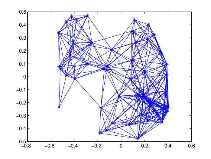
In this section, we illustrate the difference using the proposed algorithm. Consider the following EDM completion problem coming from wireless sensor networks (Figure 4). The iterates generated by the inexact Newton method are plotted in Figure 5.

Let us consider first the maximal trace solution . In Figure 6, the asterisks indicate the true locations of points in both pictures. In the picture on the left, the pluses indicate the points corresponding to the maximal trace solution after projecting onto rank PSD matrices, while in the picture on the right they denote the locations of these points after local refinement. The edges indicate the deviations.

In contrast, we now examine the minimal trace solution, Figure 7. Notice that even after a local refinement stage, the realization is very far from the true realization that we seek, an indication that a local search algorithm has converged to an extraneous critical point of the least squares objective. We have found this type of behavior to be very typical in our numerical experiments.

Finally we mention an interesting difference between the maximal trace and the minimal trace solutions as far the as the value function is concerned. When , the typical picture of the graph of is illustrated in Figure 8.

The different shapes of the curve on the left and on the right sides are striking. To elucidate this phenomenon, consider the primal problem
| minimize | |||
| subject to |
and its dual
| maximize | |||
| subject to |
In particular, the dual is strictly feasible and hence there is no duality gap. On the other hand, suppose that the dual optimal value is attained by some pair and suppose without loss of generality that has an eigenvalue equal to one corresponding to an eigenvector orthogonal to . Then letting be the optimal value (the minimal trace), and appealing to equation (16) we deduce
Hence the fact that slope is close to zero in Figure 8 indicates that the dual problem is either unattained (not surprising since the primal fails the Slater condition) or that the dual is attained only by vectors of very large magnitude. The reason why such phenomenon does not occur for the max-trace problem is an intriguing subject for further investigation.
4.4 Numerical illustration.
In this section, we illustrate the proposed method on sensor network localization instances. The data was generated in the same manner as the numerical experiments in Section 3.3. The following tables illustrate the outcome of the method by varying the noise factor (), the radio range (), and the number of sensors (). Throughout we have fixed the tolerance on the misfit . We report the density of the graph, the CPU time that our algorithms runs, the number of the Frank-Wolfe iterations (FW#), the RMSD of the resulting configuration, the RMSD of the configuration after local refinement, and the CPU time that the local refinement algorithm takes. The tests were run on MATLAB version R2011b, on a Linux machine with an Intel(R) Xeon(R) CPU E3-1225 @ 3.10GHz and 12 GB RAM.
| density | CPU | FW# | RMSD %R | RMSD %R | Refine | |||
| time (s) | initial | refined | time (s) | |||||
| 1000 | 0.0 | 0.10 | 2.9% | 9.2 | 181 | 36.3% | 0.1% | 1.2 |
| 1000 | 0.1 | 0.10 | 2.9% | 8.8 | 147 | 59.6% | 3.6% | 1.2 |
| 1000 | 0.2 | 0.10 | 2.9% | 7.3 | 136 | 89.6% | 7.5% | 1.2 |
| 1000 | 0.3 | 0.10 | 2.9% | 7.9 | 140 | 115.1% | 11.8% | 1.2 |
| 1000 | 0.1 | 0.10 | 2.9% | 8.9 | 147 | 59.6% | 3.6% | 1.2 |
| 1000 | 0.1 | 0.15 | 6.3% | 6.6 | 176 | 22.6% | 2.1% | 1.1 |
| 1000 | 0.1 | 0.20 | 10.7% | 12.4 | 356 | 11.5% | 1.4% | 1.3 |
| 1000 | 0.1 | 0.25 | 15.9% | 20.3 | 586 | 7.3% | 1.2% | 1.6 |
| 1000 | 0.1 | 0.30 | 22.0% | 45.0 | 1074 | 4.9% | 0.9% | 1.4 |
| 1000 | 0.2 | 0.10 | 2.9% | 7.3 | 136 | 89.6% | 7.5% | 1.2 |
| 2000 | 0.2 | 0.10 | 2.9% | 17.1 | 169 | 66.3% | 4.7% | 5.0 |
| 3000 | 0.2 | 0.10 | 2.9% | 30.8 | 189 | 56.4% | 3.5% | 5.0 |
| 4000 | 0.2 | 0.08 | 1.9% | 63.8 | 227 | 80.6% | 3.7% | 11.6 |
| 5000 | 0.2 | 0.08 | 1.9% | 75.1 | 179 | 74.0% | 3.3% | 16.9 |
| 6000 | 0.2 | 0.08 | 1.9% | 179.6 | 264 | 68.3% | 3.0% | 26.9 |
| 7000 | 0.2 | 0.06 | 1.1% | 253.7 | 345 | 119.1% | 4.2% | 28.8 |
| 8000 | 0.2 | 0.06 | 1.1% | 355.4 | 370 | 112.0% | 3.5% | 25.8 |
| 9000 | 0.2 | 0.06 | 1.1% | 425.8 | 338 | 108.0% | 3.4% | 42.4 |
| 10000 | 0.2 | 0.06 | 1.1% | 611.9 | 408 | 101.9% | 3.1% | 55.1 |
| 11000 | 0.2 | 0.05 | 0.8% | 744.9 | 435 | 149.3% | 3.8% | 39.5 |
| 12000 | 0.2 | 0.05 | 0.8% | 981.4 | 498 | 143.1% | 3.9% | 36.1 |
| 13000 | 0.2 | 0.05 | 0.8% | 1240.6 | 526 | 138.4% | 4.5% | 67.3 |
| 14000 | 0.2 | 0.05 | 0.8% | 1219.4 | 468 | 131.8% | 6.7% | 80.4 |
| 15000 | 0.2 | 0.05 | 0.8% | 1518.8 | 490 | 131.0% | 5.1% | 89.2 |
5 Conclusion and work in progress.
In this paper, we described two algorithms (robust facial reduction and a search along the Pareto frontier) to solve the EDM completion problem with possibly inaccurate distance measurements, which has important applications and is numerically challenging. The two algorithms are intended for EDM completion problems of different densities: the Pareto frontier algorithm discussed in Section 4 is designed for sparse graphs whereas the robust facial reduction outlined in Algorithm 1 in Section 3 tends to work better for denser graphs. Though not studied in this work, it is possible to develop a distributed implementation of the robust facial reduction technique in order to solve even larger scale completion problems. The Pareto frontier estimation technique is promising for handling large scale EDM completion problems, since first-order methods become immediately applicable and sparsity of the underlying graph can be exploited when searching for a maximum eigenvalue-eigenvector pair via a Lanczos procedure. Numerical experiments have illustrated the effectiveness of both strategies.
Appendix A Nearest-point mapping to
We now describe how to evaluate the nearest-point-mapping to the set —an easy and standard operation due to the Eckart-Young Theorem. To describe this operation, consider any matrix and a set . Define the distance function and the projection, respectively:
In this notation, we would like to find a matrix in the set . To this end, let be any orthogonal matrix. First dealing with the centering constraint, one can verify
On the other hand, we have
where are the eigenvalues of and the subscript refers to their positive part, and is any orthogonal matrix in the eigenvalue decomposition . Thus computing a matrix in requires no more than an eigenvalue decomposition.
Appendix B Solving the small least squares problem
We now describe how to easily solve the least squares system (8). Typically, the matrix will have rank . Then the face can be written as , where the matrix has as columns an orthonormal basis for the kernel of . Consequently we are interested in solving an optimization problem of the form
| s.t. |
where the linear operator is defined by for all . Let be the vectorization of and let be a matrix representation of the operator . Thus we are interested in solving the system
| (18) | ||||
| s.t. |
where is a tall-skinny matrix. One approach now is simply to expand the objective
and then apply any standard iterative method to solve the problem (18). Alternatively, one may first form an economic QR factorization (where has orthonormal columns and is upper triangular) and then write the objective as . We can then pose the problem (18) as a small linear optimization problem over the product of the semidefinite cone and a small second-order cone of dimension , and quickly solve it by an off-the-shelf Interior Point Method.
In practice, very often the cone constraint in (8) is inactive. The reason is that under reasonable conditions (see Theorem 2.2), in a noiseless situation, there is a unique solution to the equation , which happens to be positive definite. Hence by the robustness guarantees (Theorem C.5) a small amount of noise in will lead to a matrix solving that is automatically positive definite. Heuristically, we can simply drop the cone constraint in (8) and consider the unconstrained least squares problem
| (19) |
which can be solved very efficiently by classical methods. With this observation, we often can solve (8) without using any optimization software.
Appendix C Robustness of facial reduction
In this section, we provide rudimentary robustness guarantees on the Algorithm 1. To this end, consider two matrices and , each with orthonormal columns. Then the principal angles between and are the arccosines of the singular values of . We will denote the vector of principal angles between these subspaces, arranged in nondecreasing order, by . The symbols and will have obvious meanings. Thus the vector of singular values , arranged in nondecreasing order, coincides with . Consequently in terms of the matrix
the eigenvalue vector coincides with . An important property is that the principal angles between and and the principal angles between and , coincide modulo extra angles that appear for dimensional reasons. The following is a deep result that is fundamental to our analysis [14, 13, 15]. It estimates the deviation in range spaces of matrices that are nearby in norm.
Theorem C.1 (Distances and principal angles).
Consider two matrices of rank and let be the vector of principal angles between and . Then the inequality
where .
The following is immediate now.
Corollary C.2 (Deviation in exposing vectors).
Consider two rank matrices and let and be matrices with orthonormal columns that span and respectively. Then we have
Proof.
Observe . Applying Theorem C.1, the result follows. ∎
Next, we will need the following lemma.
Lemma C.3 (Projections onto subsets of symmetric matrices).
For any -matrix with orthonormal columns, and a matrix , we have
| (20) |
and for any subset , we have
| (21) |
Proof.
Optimality conditions for the optimization problem
immediately imply . Since is contained in the linear space , the projection factors into a composition
Combining this with equation (20) we deduce
On the other hand, since the columns of are orthonormal, for any we clearly have
and equation (21) follows immediately. ∎
Corollary C.4 (Distances between faces).
Consider two matrices and , each with orthonormal columns and let be the vector of principal angles between and . Then for any the estimate holds:
Proof.
Appealing to Lemma C.3, we obtain the equation . Define now the matrix . We successively deduce
Hence we deduce
The result follows. ∎
We are now ready to formally prove robustness guarantees on the method. For simplicity, we will assume that the exposing matrices are of the form where have orthonormal columns, and that for all cliques and all . The arguments can be easily adapted to a more general setting. For any subgraph of , we let denote the restriction of to . Following [31], the EDM completion problem is said to be uniquely -localizable if either of the equivalent conditions in Observation 2.2 holds. In what follows, let be the output of Algorithm 1 on the EDM completion problem.
Theorem C.5 (Robustness).
Suppose the following:
- •
for any clique , the subgraph on has embedding dimension ;
- •
the EDM completion problem is uniquely -localizable and Alg(d) is the realization of .
- •
the matrix obtained during the run on the noiseless problem has rank ;
Then there exist constants and so that
Proof.
Throughout the proof, we will use the hat superscript to denote the objects (e.g. , ) generated by Algorithm 1 when it is run with the distance measurements . Clearly for any , we have for any clique . Fix any such clique , and notice by our assumptions has rank . Consequently whenever is sufficiently close to . Appealing then to Corollary C.2, we deduce . Hence for all sufficiently close to . Since has rank , we deduce . Appealing to Theorem C.1, we then deduce , where is the principle angle vector between the null spaces of and . By Corollary C.4, then
The result follows. ∎
Acknowledgments. We thank Sasha Aravkin for pointing out a part of the proof of Theorem 4.1.
References
- [1] S. Al-Homidan and H. Wolkowicz, Approximate and exact completion problems for Euclidean distance matrices using semidefinite programming, Linear Algebra Appl., 406 (2005), pp. 109–141.
- [2] A. Alfakih and H. Wolkowicz, Matrix completion problems, in Handbook of semidefinite programming, vol. 27 of Internat. Ser. Oper. Res. Management Sci., Kluwer Acad. Publ., Boston, MA, 2000, pp. 533–545.
- [3] A.Y. Aravkin, J.V. Burke, and M.P. Friedlander, Variational properties of value functions, SIAM J. Optim., 23 (2013), pp. 1689–1717.
- [4] S. Aravkin, J. Burke, D. Drusvyatskiy, M.P. Friedlander, and S. Roy, Optimization over misfit-constrained sets, Preprint, (2015).
- [5] J. Aspnes, T. Eren, D.K. Goldenberg, A.S. Morse, W. Whiteley, Y.R. Yang, B.D.O. Anderson, and P.N. Belhumeur, Semidefinite programming approaches for sensor network localization with noisy distance measurements, IEEE Transactions on Automation Science and Engineering, 3 (2006), pp. 360–371.
- [6] P. Biswas, T.-C. Lian, T.-C. Wang, and Y. Ye, Semidefinite programming based algorithms for sensor network localization, ACM Trans. Sen. Netw., 2 (2006), pp. 188–220.
- [7] P. Biswas, T.-C. Liang, K.-C. Toh, , Y. Ye, and T.-C. Wang, Semidefinite programming approaches for sensor network localization with noisy distance measurements, IEEE Transactions on Automation Science and Engineering, 3 (2006), pp. 360–371.
- [8] P. Biswas, K.-C. Toh, and Y. Ye, A distributed SDP approach for large-scale noisy anchor-free graph reailzation with applications to molecular conformation, SIAM J. Sci. Comput., 30 (2008), pp. 1251–1277.
- [9] P. Biswas and Y. Ye, Semidefinite programming for ad hoc wireless sensor network localization, tech. report, Dept. of Management Science and Engineering, Stanford University, 2003.
- [10] P. Biswas and Y. Ye, Semidefinite programming for ad hoc wireless sensor network localization, in IPSN ’04: Proceedings of the 3rd international symposium on Information processing in sensor networks, New York, NY, USA, 2004, ACM, pp. 46–54.
- [11] G. Pataki D. Drusvyatskiy and H. Wolkowicz, Coordinate shadows of semi-definite and euclidean distance matrices, To appear in SIAM J. Optim., arXiv:1405.2037, (2015).
- [12] J. Dattorro, Convex Optimization & Euclidean Distance Geometry, Meboo Publishing, USA, 2005.
- [13] C. Davis, The rotation of eigenvectors by a perturbation. II, J. Math. Anal. Appl., 11 (1965), pp. 20–27.
- [14] C. Davis and W. M. Kahan, Some new bounds on perturbation of subspaces, Bull. Amer. Math. Soc., 75 (1969), pp. 863–868.
- [15] , The rotation of eigenvectors by a perturbation. III, SIAM J. Numer. Anal., 7 (1970), pp. 1–46.
- [16] V.F. Demyanov and A.M. Rubinov, Approximate methods in optimization problems, American Elsevier Publishing Co., Inc., New York, 1970.
- [17] M. Frank and P. Wolfe, An algorithm for quadratic programming, Naval Res. Logist. Quart., 3 (1956), pp. 95–110.
- [18] Z. Harchaoui, A. Juditsky, and A. Nemirovski, Conditional gradient algorithms for norm-regularized smooth convex optimization, Mathematical Programming, (2014), pp. 1–38.
- [19] T.L. Hayden, J. Lee, J. Wells, and P. Tarazaga, Block matrices and multispherical structure of distance matrices, Linear Algebra Appl., 247 (1996), pp. 203–216.
- [20] T.L. Hayden, J. Wells, W-M. Liu, and P. Tarazaga, The cone of distance matrices, Linear Algebra Appl., 144 (1991), pp. 153–169.
- [21] M. Jaggi, Revisiting Frank-Wolfe: Projection-free sparse convex optimization, in Proceedings of the 30th International Conference on Machine Learning (ICML-13), 2013, pp. 427–435.
- [22] N. Krislock, Semidefinite Facial Reduction for Low-Rank Euclidean Distance Matrix Completion, PhD thesis, University of Waterloo, 2010.
- [23] N. Krislock and H. Wolkowicz, Explicit sensor network localization using semidefinite representations and facial reductions, SIAM J. Optim., 20 (2010), pp. 2679–2708.
- [24] H. Kurata and P. Tarazaga, Multispherical Euclidean distance matrices, Linear Algebra Appl., 433 (2010), pp. 534–546.
- [25] , Majorization for the eigenvalues of Euclidean distance matrices, Linear Algebra Appl., 436 (2012), pp. 1473–1481.
- [26] M. Laurent, A tour d’horizon on positive semidefinite and Euclidean distance matrix completion problems, in Topics in semidefinite and interior-point methods (Toronto, ON, 1996), Amer. Math. Soc., Providence, RI, 1998, pp. 51–76.
- [27] L. Liberti, C. Lavor, N. Maculan, and A. Mucherino, Euclidean distance geometry and applications, SIAM Review, 56 (2014), pp. 3–69.
- [28] T.K. Pong and P. Tseng, Robust edge-based semidefinite programming relaxation of sensor network localization, tech. report, U. of Washington, 2009.
- [29] J.B. Saxe, Embeddability of weighted graphs in -space is strongly NP-hard, in Seventeenth Annual Allerton Conference on Communication, Control, and Computing, Proceedings of the Conference held in Monticello, Ill., October 10–12, 1979, Urbana, 1979, University of Illinois Department of Electrical Engineering, pp. xiv+1036. Proceedings of the International School of Physics “Enrico Fermi”, LXX*.
- [30] A. Singer, A remark on global positioning from local distances, Proc. Natl. Acad. Sci. USA, 105 (2008), pp. 9507–9511.
- [31] A.M. So and Y. Ye, Theory of semidefinite programming for sensor network localization, Math. Program., 109 (2007), pp. 367–384.
- [32] A. M-C So and Y. Ye, Theory of semidefinite programming for sensor network localization, Math. Program. Ser. B, (2007), pp. 367–384.
- [33] P. Tarazaga, Faces of the cone of Euclidean distance matrices: characterizations, structure and induced geometry, Linear Algebra Appl., 408 (2005), pp. 1–13.
- [34] P. Tarazaga and J.E. Gallardo, Euclidean distance matrices: new characterization and boundary properties, Linear Multilinear Algebra, 57 (2009), pp. 651–658.
- [35] P. Tarazaga, T.L. Hayden, and J. Wells, Circum-Euclidean distance matrices and faces, Linear Algebra Appl., 232 (1996), pp. 77–96.
- [36] P. Tarazaga, B. Sterba-Boatwright, and K. Wijewardena, Euclidean distance matrices: special subsets, systems of coordinates and multibalanced matrices, Comput. Appl. Math., 26 (2007), pp. 415–438.
- [37] E. van den Berg and M.P. Friedlander, SPGL1: A solver for large-scale sparse reconstruction, http://www.cs.ubc.ca/labs/scl/spgl1, (2007).
- [38] E. van den Berg and M.P. Friedlander, Probing the Pareto frontier for basis pursuit solutions, SIAM J. Sci. Comput., 31 (2008/09), pp. 890–912.
- [39] , Sparse optimization with least-squares constraints, SIAM J. Optim., 21 (2011), pp. 1201–1229.
- [40] Z. Wang, S. Zheng, Y. Ye, and S. Boyd, Further relaxations of the semidefinite programming approach to sensor network localization, SIAM J. Optim., (2008), pp. 655–673.
- [41] K.Q. Weinberger, F. Sha, and L.K. Saul, Learning a kernel matrix for nonlinear dimensionality reduction, in ICML ’04: Proceedings of the twenty-first international conference on Machine learning, New York, NY, USA, 2004, ACM, p. 106.
- [42] Y. Yemini, Some theoretical aspects of position-location problems, in 20th Annual Symposium on Foundations of Computer Science (San Juan, Puerto Rico, 1979), IEEE, New York, 1979, pp. 1–8.