Scalable Nonparametric Bayesian Inference on Point Processes with Gaussian Processes

Yves-Laurent Kom Samo Stephen Roberts Address: Deparment of Engineering Science and Oxford-Man Institute, University of Oxford

Abstract

In this paper we propose an efficient, scalable non-parametric Gaussian Process model for inference on Poisson Point Processes. Our model does not resort to gridding the domain or to introducing latent thinning points. Unlike competing models that scale as $\mathcal{O}(n^{3})$ over $n$ data points, our model has a complexity $\mathcal{O}(nk^{2})$ where $k\ll n$ . We propose a MCMC sampler and show that the model obtained is faster, more accurate and generates less correlated samples than competing approaches on both synthetic and real-life data. Finally, we show that our model easily handles data sizes not considered thus far by alternate approaches.

Keywords:

Point Processes, Cox Processes, Gaussian Processes

1 INTRODUCTION

Point processes are a standard model when the objects of study are the number and repartition of otherwise identical points on a domain, usually time or space. The Poisson Point Process is probably the most commonly used point process. It is fully characterised by an intensity function that is inferred from the data. Gaussian Processes have been successfully used to form a prior over the (log-) intensity function for applications such as astronomy (Gregory & Loredo, 1992), forestry (Heikkinen & Arjas, 1999), finance (Basu & Dassios, 2002), and neuroscience (Cunningham et al., 2008b). We offer extensions to existing work as follows: we develop an exact non-parametric Bayesian model that enables inference on Poisson processes. Our method scales linearly with the number of data points and does not resort to gridding the domain. We derive a MCMC sampler for core components of the model and show that our approach offers a faster and more accurate solution, as well as producing less correlated samples, compared to other approaches on both real-life and synthetic data.

2 RELATED WORK

Non-parametric inference on point processes has been extensively studied in the literature. (Rathbum & Cressie, 1994) and (Moeller et al., 1998) used a finite-dimensional piecewise constant log-Gaussian for the intensity function. Such approximations are limited in that the choice of the grid on which to represent the intensity function is arbitrary and one has to trade-off precision with computational complexity and numerical accuracy, with the complexity being cubic in the precision and exponential in the dimension of the input space. (Kottas, 2006; Kottas & Sanso, 2007) used a Dirichlet process mixture of Beta distributions as prior for the normalised intensity function of a Poisson process. (Cunningham et al., 2008a) proposed a model using Gaussian Processes evaluated on a fixed grid for the estimation of intensity functions of renewal processes with log-concave renewal distributions. They turned hyper-parameters inference into an iterative series of convex optimization problems, where ordinarily cubic complexity operations such as Cholesky decompositions are evaluated in $\mathcal{O}(n\log{n})$ leveraging the uniformity of the grid and the log-concavity of the renewal distribution. (Adams et al., 2009) proposed an exact Markov Chain Monte Carlo (MCMC) inference scheme for the posterior intensity function of a Poisson Process with a Sigmoid Gaussian prior intensity, or equivalently a Cox Process (Cox, 1955) with Sigmoid Gaussian stochastic intensity. The authors simplified the likelihood of a Cox process by introducing latent thinning points. The proposed scheme has a complexity exponential in the dimension of the input space, cubic in the number of data and thinning points, and performs particularly poorly when the data are sparse. (Gunter et al., 2014) extended this model to structured point processes. (Rao & Teh, 2011) used uniformization to produce exact samples from a non-stationary renewal process whose hazard function is modulated by a Gaussian Process, and consequently proposed an MCMC sampler to sample from the posterior intensity of a unidimensional point process. Although the authors have illustrated that their model is faster than (Adams et al., 2009) on some synthetic and real-life data, their method still scales cubically in the number of thinned and data points, and is not applicable to data in dimension higher than 1, such as spatial point processes.

3 MODEL

3.1 Setup

We are tasked with making non-parametric Bayesian inference on the intensity function of a Poisson Point Process assumed to have generated a dataset $\mathcal{D}=\{s_{1},...,s_{n}\}$ . To simplify the discourse without loss of generality, we will assume that data points take values in $\mathbb{R}^{d}$ .

Firstly, let us recall that a Poisson Point Process (PPP) on a bounded domain $\mathcal{S}\subset\mathbb{R}^{d}$ with non-negative intensity function $\lambda$ is a locally finite random collection of points in $\mathcal{S}$ such that the numbers of points occurring in disjoint parts $B_{i}$ of $\mathcal{S}$ are independent and each follows a Poisson distribution with mean $\int_{B_{i}}\lambda(s)ds$ .

The likelihood of a PPP is given by:

\displaystyle L(\lambda|s_{1},...,s_{n})=\exp\left(-\int_{\mathcal{S}}\lambda(s)ds\right)\prod_{i=1}^{n}\lambda(s_{i})

(1)

3.2 Tractability discussion

The approach adopted thus far in the literature to make non-parametric Bayesian inference on Point Process using Gaussian Processes (GP) (Rassmussen & Williams, 2006) consists of putting a functional prior on the intensity function in the form of a positive function of a GP: $\lambda(s)=f(g(s))$ where $g$ is drawn from a GP and $f$ is a positive function. Examples of such $f$ include the exponential function and a scaled sigmoid function (Adams et al., 2009; Rao & Teh, 2011). This approach can be seen as a Cox Process where the stochastic intensity follows the same dynamics as the functional prior. When the Gaussian Process used has almost surely continuous paths, the random vector

\displaystyle(\lambda(s_{1}),...,\lambda(s_{n}),\int_{\mathcal{S}}\lambda(s)ds)

(2)

provably admits a probability density function (pdf). Moreover, we note that any piece of information not contained in the implied pdf over the vector in Equation (2) will be lost as the likelihood only depends on those variables. Hence, given a functional prior postulated on the intensity function, the only necessary piece of information to be able to make a full Bayesian treatment is the implied joint pdf over the vector in Equation (2).

For many useful transformations $f$ and covariance structures for the GP, the aforementioned implied pdf might not be available analytically. We note however that there is no need to put a functional prior on the intensity function. In fact, for every finite-dimensional prior over the vector in Equation (2), there exists a Cox process with an a.s. $\mathcal{C}^{\infty}$ intensity process that coincides with the postulated prior (see appendix for the proof).

This approach is similar to that of (Kottas, 2006). The author regarded $I=\int_{\mathcal{S}}\lambda(s)ds$ as a random variable and noted that $p(s)=\frac{\lambda(s)}{\int_{\mathcal{S}}\lambda(s)ds}$ can be regarded as a pdf whose support is the domain $\mathcal{S}$ . He then made inference on $(I,p(s_{1}),...,p(s_{n}))$ , postulating as prior that $I$ and $(p(s_{1}),...,p(s_{n}))$ are independent, $I$ has a Jeffreys prior and $(s_{1},...,s_{n})$ are i.i.d. draws from a Dirichlet Process mixture of Beta with pdf $p$ .

The model we present in the following section puts an appropriate finite-dimensional prior on $(\lambda(s_{1}),...,\lambda(s_{n}),\lambda(s^{\prime}_{1}),...,\lambda(s^{\prime}_{k}),\int_{\mathcal{S}}\lambda(s)ds)$ for some inducing points $s^{\prime}_{j}$ rather than putting a functional prior on the intensity function directly.

3.3 Our model

3.3.1 Intuition

The intuition behind our model is that the data are not a ‘natural grid’ at which to infer the value of the intensity function. For instance, if the data consists of 200,000 points on the interval $[0,24]$ as in one of our experiments, it might not be necessary to infer the value of a function at 200,000 points to characterise it on $[0,24]$ . Instead, we find a small set of inducing points $\mathcal{D}^{\prime}=\{s^{\prime}_{1},...,s^{\prime}_{k}\},k\ll n$ on our domain, through which we will define the prior over the vector in Equation (2) augmented with $\lambda(s^{\prime}_{1}),...,\lambda(s^{\prime}_{k})$ . The set of inducing points will be chosen so that knowing $\lambda(s^{\prime}_{1}),...,\lambda(s^{\prime}_{k})$ would result in knowing the values of the intensity function elsewhere on the domain, in particular $\lambda(s_{1}),...,\lambda(s_{n})$ , with ‘arbitrary certainty’. We will then analytically integrate out the dependency in $\lambda(s_{1}),...,\lambda(s_{n})$ from the posterior, thereby reducing the complexity from cubic to linear in the number of data points without ‘loss of information’, and reformulating our problem as that of making exact Bayesian inference on the value of the intensity function at the inducing points. We will then describe how to obtain predictive mean and variance of the intensity function elsewhere on the domain from training.

3.3.2 Model specification

Let us denote by $\lambda^{*}$ a positive stochastic process on $\mathcal{S}$ such that $\log{\lambda^{*}}$ is a stationary Gaussian Process with covariance kernel $\gamma^{*}:(s_{1},s_{2})\to\gamma^{*}(s_{1},s_{2})$ and constant mean $m^{*}$ . Let us further denote by $\hat{\lambda}$ a positive stochastic process on $\mathcal{S}$ such that $\log{\hat{\lambda}}$ is a Conditional Gaussian Process coinciding with $\log{\lambda^{*}}$ at $k$ inducing points $\mathcal{D}^{\prime}=\{s^{\prime}_{1},...,s^{\prime}_{k}\},k\ll n$ . That is, $\log{\hat{\lambda}}$ is the non-stationary Gaussian Process whose mean function $m$ is defined by

\displaystyle m(s)=m^{*}+\Sigma^{*}_{s\mathcal{D}^{\prime}}\Sigma^{*-1}_{\mathcal{D}^{\prime}\mathcal{D}^{\prime}}G

(3)

where $G=\big(\log{\lambda^{*}(s^{\prime}_{1})}-m^{*},...,\log{\lambda^{*}(s^{\prime}_{k})}-m^{*}\big)$ and $\Sigma^{*}_{XY}$ is the covariance matrix between the vectors $X$ and $Y$ under the covariance kernel $\gamma^{*}$ . Moreover, $\log{\hat{\lambda}}$ is such that for every vector $S_{1}$ of points in $\mathcal{S}$ , the auto-covariance matrix $\Sigma_{S_{1}S_{1}}$ of the values of process at $S_{1}$ reads¹¹ 1 The positive definitiveness of the induced covariance kernel $\gamma$ is a direct consequence of the positive definitiveness of $\gamma^{*}$ .

\displaystyle\Sigma_{S_{1}S_{1}}=\Sigma^{*}_{S_{1}S_{1}}-\Sigma^{*}_{S_{1}\mathcal{D}^{\prime}}\Sigma^{*-1}_{\mathcal{D}^{\prime}\mathcal{D}^{\prime}}\Sigma^{*T}_{S_{1}\mathcal{D}^{\prime}}.

(4)

The prior distribution in our model is constructed as follows:

1.

$\{\log{\lambda(s^{\prime}_{i})}\}_{i=1}^{k}$ are samples from the stationary GP $\log{\lambda^{*}}$ at $\{s^{\prime}_{i}\}_{i=1}^{k}$ respectively, with $m^{*}=\log{\frac{\#\mathcal{D}}{\mu(\mathcal{S})}}$ , where $\mu(\mathcal{S})$ is the size of the domain.
2.

$I=\int_{\mathcal{S}}\lambda(s)ds$ and $\{\log{\lambda(s_{j})}\}_{j=1}^{n}$ are conditionally independent given $\{\log{\lambda(s^{\prime}_{i})}\}_{i=1}^{k}$ .
3.

Conditional on $\{\log{\lambda(s^{\prime}_{i})}\}_{i=1}^{k}$ , $\{\log{\lambda(s_{j})}\}_{j=1}^{n}$ are independent, and for each $j\in[1..n]$ $\log{\lambda(s_{j})}$ follows the same distribution as $\log{\hat{\lambda}(s_{j})}$ .
4.

Conditional on $\{\log{\lambda(s^{\prime}_{i})}\}_{i=1}^{k}$ , $I$ follows a Gamma distribution with shape $\alpha_{I}$ and scale $\beta_{I}$ .
5.

The mean $\mu_{I}=\alpha_{I}\beta_{I}$ and variance $\sigma^{2}_{I}=\alpha_{I}\beta_{I}^{2}$ of $I$ are that of $\int_{\mathcal{S}}\hat{\lambda}(s)ds$ .

Assertion 3. above is somewhat similar to the FITC model of (Quinonero & Rasmussen, 2005).

This construction yields a prior pdf of the form:

		$\displaystyle p\big(\log{\lambda(s_{1})},...,\log{\lambda(s_{n})},\log{\lambda(s^{\prime}_{1})},...,\log{\lambda(s^{\prime}_{k})},I,\theta\big)$
		$\displaystyle=\mathcal{N}\big(\log{\lambda(s^{\prime}_{1})},...,\log{\lambda(s^{\prime}_{k})}\rvert m^{}1_{k},\Sigma^{}_{\mathcal{D}^{\prime}\mathcal{D}^{\prime}}\big)$
		$\displaystyle\times\mathcal{N}\big(\log{\lambda(s_{1})},...,\log{\lambda(s_{n})}\rvert M,\text{diag}(\Sigma_{\mathcal{D}\mathcal{D}})\big)$
		$\displaystyle\times\gamma_{d}\big(I\rvert\alpha_{I},\beta_{I}\big)\times p(\theta)$		(5)

where $\mathcal{N}(.\rvert X,C)$ is the multivariate Gaussian pdf with mean $X$ and covariance matrix $C$ , $M=(m(s_{1}),...,m(s_{n}))$ , $1_{k}$ is the vector with length k and elements 1, $\text{diag}(\Sigma_{\mathcal{D}\mathcal{D}})$ is the diagonal matrix whose diagonal is that of $\Sigma_{\mathcal{D}\mathcal{D}}$ , $\gamma_{d}\big(x\rvert\alpha,\beta)$ is the pdf of the gamma distribution with shape $\alpha$ and scale $\beta$ , and where $\theta$ denotes the hyper-parameters of the covariance kernel $\gamma^{*}$ .

It follows from the fifth assertion in our prior specification that $\alpha_{I}=\frac{\mu_{I}^{2}}{\sigma_{I}^{2}}\text{ and }\beta_{I}=\frac{\sigma_{I}^{2}}{\mu_{I}}$ . We also note that

$\displaystyle\mu_{I}$	$\displaystyle=\text{E}\big(\int_{\mathcal{S}}\hat{\lambda}(s)ds\big)$
	$\displaystyle=\int_{\mathcal{S}}\text{E}\big(\exp(\log{\hat{\lambda}(s)})\big)ds$
	$\displaystyle=\int_{\mathcal{S}}\exp(m(s)+\frac{1}{2}\gamma(s,s))ds$	$\displaystyle:=\int_{\mathcal{S}}f(s)ds$	(6)

and

$\displaystyle\sigma_{I}^{2}$	$\displaystyle=\text{E}\bigg(\big(\int_{\mathcal{S}}\hat{\lambda}(s)ds\big)^{2}\bigg)-\mu_{I}^{2}$
	$\displaystyle=\text{E}\bigg(\int_{\mathcal{S}}\int_{\mathcal{S}}\exp(\log{\hat{\lambda}(s_{1})}+\log{\hat{\lambda}(s_{2})})ds_{1}ds_{2}\bigg)-\mu_{I}^{2}$
	$\displaystyle=\int_{\mathcal{S}}\int_{\mathcal{S}}\text{E}\bigg(\exp\big(\log{\hat{\lambda}(s_{1})}+\log{\hat{\lambda}(s_{2})}\big)\bigg)ds_{1}ds_{2}-\mu_{I}^{2}$
	$\displaystyle=\int_{\mathcal{S}}\int_{\mathcal{S}}\exp\big(m(s_{1})+m(s_{2})+\gamma(s_{1},s_{2})+\frac{1}{2}\gamma(s_{1},s_{1})$
	$\displaystyle+\frac{1}{2}\gamma(s_{2},s_{2})\big)ds_{1}ds_{2}-\mu_{I}^{2}$
	$\displaystyle:=\int_{\mathcal{S}}\int_{\mathcal{S}}g(s_{1},s_{2})ds_{1}ds_{2}-\mu_{I}^{2}.$	(7)

The integrals in Equations (6) and (7) can be easily evaluated with numerical methods such as Gauss-Legendre quadrature (Hildebrand, 2003).

In particular, when $\mathcal{S}=[a,b]$ ,

\displaystyle\mu_{I}\approx\frac{b-a}{2}\sum_{i=1}^{p}\omega_{i}f\left(\frac{b-a}{2}x_{i}+\frac{b+a}{2}\right)

(8)

and

		$\displaystyle\sigma_{I}^{2}\approx\frac{(b-a)^{2}}{4}\sum_{i=1}^{p}\sum_{j=1}^{p}\omega_{i}\omega_{j}g\Big(\frac{b-a}{2}x_{i}+\frac{b+a}{2},\frac{b-a}{2}x_{j}+$
		$\displaystyle\frac{b+a}{2}\Bigg)-\mu_{I}^{2}$		(9)

where the roots $x_{i}$ of the Legendre polynomial of order $p$ and the weights $\omega_{i}$ are readily available from standard textbooks on numerical analysis such as (Hildebrand, 2003) and scientific programming packages (R, Matlab and Scipy). Extensions to rectangles in higher dimensions are straightforward. Moreover, the complexity of such approximations only depends on the number of inducing points and $p$ (see Equations (3) and (4)), and hence scales well with the data size.

A critical step in the derivation of our model is to analytically integrate out $\log{\lambda(s_{1})},...,\log{\lambda(s_{n})}$ in the posterior, to eliminate the cubic complexity in the number of data points. To do so, we note that:

		$\displaystyle\int_{(\mathbb{R}^{d})^{n}}\prod_{i=1}^{n}\lambda(s_{i})\mathcal{N}\big(\log{\lambda(s_{1})},...,\log{\lambda(s_{n})}\rvert M,$
		$\displaystyle\text{diag}(\Sigma_{\mathcal{D}\mathcal{D}})\big)d\log{\lambda(s_{1})}...d\log{\lambda(s_{n})}$
		$\displaystyle=\text{E}\left(\exp\left(\sum_{i=1}^{n}\log{\lambda(s_{i})}\right)\right)$
		$\displaystyle=\exp(1_{n}^{T}M+\frac{1}{2}\text{Tr}(\Sigma_{\mathcal{D}\mathcal{D}}))$		(10)

where the second equality results from the moment generating function of a multivariate Gaussian.

Thus, putting together the likelihood of Equation (1) and Equation (5), and integrating out $\big(\log{\lambda(s_{1})},...,\log{\lambda(s_{n})}\big)$ , we get:

		$\displaystyle p\big(\log{\lambda(s^{\prime}_{1})},...,\log{\lambda(s^{\prime}_{k})},I,\theta\big\rvert\mathcal{D})$
		$\displaystyle\sim p(\theta)\mathcal{N}\big(\log{\lambda(s^{\prime}_{1})},...,\log{\lambda(s^{\prime}_{k})}\rvert M^{},\Sigma^{}_{\mathcal{D}^{\prime}\mathcal{D}^{\prime}}\big)$
		$\displaystyle\times\exp(1_{n}^{T}M+\frac{1}{2}\text{Tr}(\Sigma_{\mathcal{D}\mathcal{D}}))\exp(-I)\gamma_{d}\big(I\rvert\alpha_{I},\beta_{I}\big)$		(11)

Finally, although our model allows for joint inference on the intensity function and its integral, we restrict our attention to making inference on the intensity function for brevity. By integrating out $I$ from Equation (11), we get the new posterior:

$\displaystyle p(\lambda,\theta\rvert\mathcal{D})$	$\displaystyle:=p\big(\log{\lambda(s^{\prime}_{1})},...,\log{\lambda(s^{\prime}_{k})},\theta\big\rvert\mathcal{D})$	(12)
	$\displaystyle\sim p(\theta)\exp(1_{n}^{T}M+\frac{1}{2}\text{Tr}(\Sigma_{\mathcal{D}\mathcal{D}}))(1+\beta_{I})^{-\alpha_{I}}$
	$\displaystyle\times\mathcal{N}\big(\log{\lambda(s^{\prime}_{1})},...,\log{\lambda(s^{\prime}_{k})}\rvert M^{},\Sigma^{}_{\mathcal{D}^{\prime}\mathcal{D}^{\prime}}\big)$

where we noted that the dependencies of Equation (11) in $I$ is of the form $\exp(-x)\gamma_{d}(x\rvert\alpha,\beta)$ which can be integrated out as the moment generating function of the gamma distribution evaluated at $-1$ , that is $(1+\beta)^{-\alpha}$ .

3.3.3 Selection of inducing points

Inferring the number $k$ and positions of the inducing points $s^{\prime}_{i}$ is critical to our model, as $k$ directly affects the complexity of our scheme and the positions of the inducing points affect the quality of our prediction. Too large a $k$ will lead to an unduly large complexity. Too small a $k$ will lead to loss of information (and subsequently excessively uncertain predictions from training), and might make assertion 2 of our prior specification inappropriate. For a given $k$ , if the inducing points are not carefully chosen, the coverage of the domain will not be adapted to changes in the intensity function and as a result, the predictive variance in certain parts of the domain might considerably differ from the posterior variance we would have obtained, had we chosen inducing points in those parts of the domain.

Intuitively, a good algorithm to find inducing points should leverage prior knowledge about the smoothness, periodicity, amplitude and length scale(s) of the intensity function to optimize for the quality of (post-training) predictions while minimising the number of inducing points.

We use as utility function for the choice of inducing points:

\displaystyle\mathcal{U}(\mathcal{D}^{\prime})=\text{E}_{\theta}(\text{Tr}(\Sigma_{\mathcal{D}\mathcal{D}^{\prime}}^{*}(\theta)\Sigma_{\mathcal{D^{\prime}}\mathcal{D^{\prime}}}^{*-1}(\theta)\Sigma_{\mathcal{D}\mathcal{D}^{\prime}}^{*T}(\theta)))

(13)

where $\theta$ is the vector of hyper-parameters of the covariance kernel $\gamma^{*}$ , and the expectation is taken with respect to the prior distribution over $\theta$ . In other words, the utility of a set of inducing points is the expected total reduction of the (predictive) variances of $\log{\lambda(s_{1})},...\log{\lambda(s_{n})}$ resulting from knowing $\log{\lambda(s^{\prime}_{1})},...,\log{\lambda(s^{\prime}_{k})}$ .

In practice, the expectation in Equation (13) might not be available analytically. We can however use the Monte Carlo estimate:

\displaystyle\tilde{\mathcal{U}}(\mathcal{D}^{\prime})

\displaystyle=\frac{1}{N}\sum_{i=1}^{N}\text{Tr}(\Sigma_{\mathcal{D}\mathcal{D}^{\prime}}^{*}(\tilde{\theta}_{i})\Sigma_{\mathcal{D^{\prime}}\mathcal{D^{\prime}}}^{*-1}(\tilde{\theta}_{i})\Sigma_{\mathcal{D}\mathcal{D}^{\prime}}^{*T}(\tilde{\theta}_{i})).

(14)

The algorithm proceeds as follows. We sample $(\tilde{\theta}_{i})_{i=1}^{N}$ from the prior. Initially we set $k=0$ , $\mathcal{D}^{\prime}=\varnothing$ and $u_{0}=0$ . We increment $k$ by one, and consider adding an inducing point. We then find the point $s_{k}^{\prime}$ that maximises $\tilde{\mathcal{U}}(\mathcal{D}^{\prime}\cup\{s\})$

\displaystyle s_{k}^{\prime}:=\underset{s\in\mathcal{S}}{\text{argmax }}\tilde{\mathcal{U}}(\mathcal{D}^{\prime}\cup\{s\})

(15)

using Bayesian optimisation (Mockus, 2013). We compute the utility of having $k$ inducing points as

u_{k}=\tilde{\mathcal{U}}(\mathcal{D}^{\prime}\cup\{s_{k}^{\prime}\}),

we update $\mathcal{D}^{\prime}=\mathcal{D}^{\prime}\cup\{s_{k}\}$ and stop when

\frac{u_{k}-u_{k-1}}{u_{k}}<\alpha,

where $0<\alpha\ll 1$ is a convergence threshold.

Algorithm 1 Selection of inducing points

Inputs:

0<\alpha\ll 1

N

p_{\theta}

Output:

u_{f}

\mathcal{D}^{\prime}

k=0

u_{0}=0

\mathcal{D}^{\prime}=\varnothing

e=1

;

Sample

(\tilde{\theta}_{i})_{i=1}^{N}

from

p(\theta)

;

while

e>\alpha

k=k+1;

s^{\prime}_{k}=\underset{s\in\mathcal{S}}{\text{argmax }}\tilde{\mathcal{U}}(\mathcal{D}^{\prime}\cup\{s\});

u_{k}=\tilde{\mathcal{U}}(\mathcal{D}^{\prime}\cup\{s^{\prime}_{k}\});

\mathcal{D}^{\prime}=\mathcal{D}^{\prime}\cup\{s^{\prime}_{k}\};

e=\frac{u_{k}-u_{k-1}}{u_{k}};

end while

Proposition

(a) For any $\mathcal{D}$ , $\alpha$ , $N$ and $p_{\theta}$ Algorithm 1 stops in finite time and the sequence $(u_{k})_{k\in\mathbb{N}}$ converges at least linearly with rate $1-\frac{1}{\#\mathcal{D}}$ .

(b) Moreover, the maximum utility $u_{f}(\alpha)$ returned by Algorithm 1 converges to the average total unconditional variance $w_{\infty}:=\frac{1}{N}\sum_{i=1}^{N}\text{Tr}(\Sigma_{\mathcal{D}\mathcal{D}}^{*}(\tilde{\theta}_{i}))$ as $\alpha$ goes to $0$ .

The idea behind the proof of this proposition is that the sequence of maximum utilities $u_{k}$ is positive, increasing²² 2 Intuitively, conditioning on a new point increases the reduction of variance from the unconditional variance., and upper-bounded by the total unconditional variance $w_{\infty}$ ³³ 3 The variance cannot be reduced by more than the total unconditional variance.. Hence, the sequence $u_{k}$ converges to a strictly positive limit, which implies that the stopping condition of the while loop will be met in finite time regardless of $\mathcal{D}$ , $\alpha$ , $N$ and $p_{\theta}$ . Finally, we construct a sequence $w_{k}$ upper-bounded by the sequence $u_{k}$ and that converges linearly to the average total unconditional variance $w_{\infty}$ with rate $1-\frac{1}{\#\mathcal{D}}$ . As the sequence $u_{k}$ converges and is itself upper-bounded by $w_{\infty}$ , its limit is $w_{\infty}$ as well, and it converges at least as fast as $w_{k}$ . (See appendix for the full proof)

Our algorithm is particularly suitable to Poisson Point Processes as it prioritises sampling inducing points in parts of the domain where the data are denser. This corresponds to regions where the intensity function will be higher, thus where the local random counts of the underlying PPP will vary more⁴⁴ 4 The variance of the Poisson distribution is its mean. and subsequently where the posterior variance of the intensity is expected to be higher. Moreover, it leverages prior smoothness assumptions on the intensity function to limit the number of inducing points and to appropriately and sequentially improve coverage of the domain.

Algorithm 1 is illustrated on a variety of real life and synthetic data sets in section 5.

4 INFERENCE

We use a Squared Exponential kernel for $\gamma^{*}$ and Scaled Sigmoid Gaussian priors for the kernel hyper-parameters; that is $\theta_{i}=\frac{\theta_{i\text{max}}}{1+\exp(-x_{i})}$ where $x_{i}$ are i.i.d standard Normal. The problem-specific scales, $\theta_{i\text{max}}$ , restrict the supports of those distributions using prior knowledge to avoid unlikely extreme values and to improve conditioning.

We use a Block Gibbs Sampler (Geman & Geman, 1984) to sample from the posterior. We sample the hyper-parameters using the Metropolis-Hastings (Hastings, 1970) algorithm taking as proposal distribution the prior of the variable of interest. We sample the log-intensities at the inducing points using Elliptical Slice Sampling (Murray et al., 2010) with the pdf in Equation (12).

Prediction from training

To predict the posterior mean at the data points we note from the law of total expectation that

		$\displaystyle\forall s_{i}\in\mathcal{D},~\text{E}(\log{\lambda(s_{i})}\|\mathcal{D})$
		$\displaystyle=\text{E}\left(\text{E}\left(\log{\lambda(s_{i})}\|\{\log{\lambda^{*}(s^{\prime}_{j})}\}_{j=1}^{k},\mathcal{D}\right)\|\mathcal{D}\right).$		(16)

Also, we note from Equations (1) and (5) that the dependency of the posterior of $\log{\lambda(s_{i})}$ conditional on $\{\log{\lambda^{*}(s^{\prime}_{j})}\}_{j=1}^{k}$ is of the form

\exp(\log{\lambda(s_{i})})\times\mathcal{N}(\log{\lambda(s_{i})}|m(s_{i}),\gamma(s_{i},s_{i})),

where we recall that $m(s_{i})$ is the $i$ -th element of the vector $M$ and $\gamma(s_{i},s_{i})$ is the $i$ -th diagonal element of the matrix $\Sigma_{\mathcal{D}\mathcal{D}}$ . Hence, the posterior distribution of $\log{\lambda(s_{i})}$ conditional on $\{\log{\lambda^{*}(s^{\prime}_{j})}\}_{j=1}^{k}$ is Gaussian with mean

\displaystyle\text{E}\left(\log{\lambda(s_{i})}|\{\log{\lambda^{*}(s^{\prime}_{j})}\}_{j=1}^{k},\mathcal{D}\right)=M[i]+\Sigma_{\mathcal{D}\mathcal{D}}[i,i]

(17)

and variance

\displaystyle\text{Var}\left(\log{\lambda(s_{i})}|\{\log{\lambda^{*}(s^{\prime}_{j})}\}_{j=1}^{k},\mathcal{D}\right)=\Sigma_{\mathcal{D}\mathcal{D}}[i,i].

(18)

Finally, it follows from Equation (16) that $\text{E}(\log{\lambda(s_{i})}|\mathcal{D})$ is obtained by averaging out $M[i]+\Sigma_{\mathcal{D}\mathcal{D}}[i,i]$ over MCMC samples after burn-in.

Similarly, the law of total variance implies that

		$\displaystyle\text{Var}(\log{\lambda(s_{i})}\|\mathcal{D})$
		$\displaystyle=\text{E}\left(\text{Var}\left(\log{\lambda(s_{i})}\|\{\log{\lambda^{*}(s^{\prime}_{j})}\}_{j=1}^{k},\mathcal{D}\right)\|\mathcal{D}\right)$
		$\displaystyle+\text{Var}\left(\text{E}\left(\log{\lambda(s_{i})}\|\{\log{\lambda^{*}(s^{\prime}_{j})}\}_{j=1}^{k},\mathcal{D}\right)\|\mathcal{D}\right).$		(19)

Hence, it follows from Equations (17) and (18) that the posterior variance at a data point $s_{i}$ is obtained by summing up the sample mean of $\Sigma_{\mathcal{D}\mathcal{D}}[i,i]$ with the sample variance of $M[i]+\Sigma_{\mathcal{D}\mathcal{D}}[i,i]$ , where sample mean and sample variance are taken over MCMC samples after burn-in.

5 EXPERIMENTS

We selected four data sets to illustrate the performance of our model. We restricted ourselves to one synthetic data set for brevity. We chose the most challenging of the synthetic intensity functions of (Adams et al., 2009) and (Rao & Teh, 2011), $\lambda(t)=2\exp(-\frac{t}{15})+\exp(-(\frac{t-25}{10})^{2})$ , to thoroughly compare our model with competing methods. We also ran our model on a standard 1 dimensional real-life data set (the coal mine disasters dataset used in (Jarrett, 1979); 191 points) and a standard real-life 2 dimensional data (spatial location of bramble canes (Diggle, 1983); 823 points). Finally we ran our model on a real-life data set large enough to cause problems to competing models. This data set consists of the UTC timestamps (expressed in hours in the day) of Twitter updates in English published in the (Twitter Sample Stream, 2014) on September 1st 2014 (188544 points).

5.1 Inducing points selection

Figure 1 illustrates convergence of the selection of inducing points on the 4 data sets. We ran the algorithm 10 times with $N=20$ , and plotted the average normalised utility $\frac{u_{k}}{u_{\infty}}\pm 1\text{ std}$ as a function of the number of inducing points. Table 1 contains the maximum hyper-parameters that were used for each data set. Table 2 contains the number of inducing points required to achieve some critical normalised utility values for each of the 4 data sets. We note that just 8 inducing points were required to achieve a 95% utility for the Twitter data set (188544 points). In regards to the positions of sampled inducing points, we note from Figures 2 and 3 that when the intensity function was bimodal, the first inducing point was sampled around the argument of the highest mode, and the second inducing point was sampled around the argument of the second highest mode. More generally, the algorithm sampled inducing points where the latent intensity function varies the most, as expected.

Table 1: Maximum output (resp. input) scale

h_{\text{max}}

(resp.

l_{\text{max}}

) used for each data set to select inducing points.

	synthetic	coal mine	bramble	twitter
$h_{\text{max}}$	10.0	10.0	10.0	10.0
$l_{\text{max}}$	25.0	50.0	0.25	5.0

Refer to caption — Figure 1: Average normalised utility $\frac{u_{k}}{u_{\infty}}$ of choosing k inducing points using Algorithm 1 $\pm$ 1 standard deviation as a function of k on the synthetic data set (eg), the coal mine data set (cm), the Twitter data set (t) and the bramble canes data set (b). The average was taken over 10 runs.

Table 2: Number of inducing points produced by Algorithm 1 required to achieve some critical normalised utility values on the 4 data sets.

	$k$
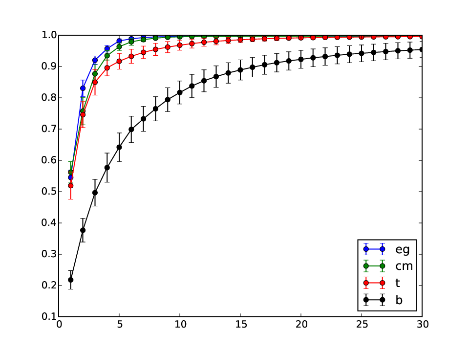
$\frac{u_{k}}{u_{\infty}}$	synthetic	coal mine	bramble	twitter
0.75	2	2	8	3
0.90	3	4	17	5
0.95	4	5	28	8

5.2 Intensity function

In each experiment we generated 5000 samples after burn-in (1000 samples). For each data set we used the set of inducing points that yielded a 95% normalized utility. The exact numbers are detailed in Table 2.

We ran a Monte Carlo simulation for the stochastic processes considered herein and found that the Legendre polynomial order $p=10$ was sufficient to yield a Quadrature estimate for the standard deviation of the integral less than 1% away from the Monte Carlo estimate (using the trapezoidal rule), and a Quadrature estimate for the mean of the integral less than a standard error away from the Monte Carlo average. We took a more conservative stand and used $p=20$ .

Inference on synthetic data

We generated a draw from a Poisson point process with the intensity function $\lambda(t)=2\exp(-\frac{t}{15})+\exp(-(\frac{t-25}{10})^{2})$ of (Adams et al., 2009) and (Rao & Teh, 2011). The draw consisted of 41 points (blue sticks in Figure 2). We compared our model to (Adams et al., 2009) (SGCP) and (Rao & Teh, 2011) (RMP). We ran the RMP model with the renewal parameter $\gamma$ set to 1 (RMP 1), which corresponds to an exponential renewal distribution or equivalently an inhomogeneous Poisson process. We also ran the RMP model with a uniform prior on $[1,5]$ over the renewal parameter $\gamma$ (RMP full). Figure 2 illustrates the posterior mean intensity function under each model. Finally we ran the Dirichlet Process Mixture of Beta model of (Kottas, 2006) (DPMB). As detailed in Table 3, our model outperformed that of (Adams et al., 2009), (Rao & Teh, 2011) and (Kottas, 2006) in terms of accuracy and speed.

Table 3: Some statistics on the MCMC runs of Figure 2. RMSE and MAE denote the Root Mean Square Error and the Mean Absolute Error, expressed as a proportion of the average of the true intensity function over the domain. LP denotes the log mean predictive probability on 10 held out PPP draws from the true intensity

\pm

1 std. t(s) is the average time in seconds it took to generate 1000 samples

\pm

1 std and ESS denotes the average effective sample size (Gelman et al., 2013) per 1000 samples.

	MAE	RMSE	LP	t (s)	ESS
SGCP	0.31	0.37	-45.07 $\pm$ 1.64	257.72 $\pm$ 16.29	6
RMP 1	0.32	0.38	-45.24 $\pm$ 1.41	110.19 $\pm$ 7.37	23
RMP full	0.25	0.31	-43.51 $\pm$ 2.15	139.64 $\pm$ 5.24	6
DPMB	0.23	0.32	-42.95 $\pm$ 3.58	23.27 $\pm$ 0.94	47
Us	0.19	0.27	-42.84 $\pm$ 3.07	4.35 $\pm$ 0.12	38

Inference on real-life data

Figure 3 shows the posterior mean intensity functions of the coal mine data set, the Twitter data set and the bramble canes data set under our model.

Scalability:

We note that it took only 240s on average to generate 1000 samples on the Twitter data set (188544 points). As a comparison, this is the amount of time that would be required to generate as many samples on a data set that has 50 points (resp. 100 points) under the models of (Adams et al., 2009) (resp. (Rao & Teh, 2011)). More importantly, it was not possible to run either of those two competing models on the twitter data set. Doing so would require computing $17\times 10^{10}$ covariance coefficients to evaluate a single auto-covariance matrix of the log-intensity at the data points, which a typical personal computer cannot handle.

6 DISCUSSION

Scalability of the selection of inducing points

The computational bottleneck of the selection of inducing points is in the evaluation of

\text{Tr}(\Sigma_{\mathcal{D}\mathcal{D}^{\prime}}^{*}(\tilde{\theta}_{i})\Sigma_{\mathcal{D^{\prime}}\mathcal{D^{\prime}}}^{*-1}(\tilde{\theta}_{i})\Sigma_{\mathcal{D}\mathcal{D}^{\prime}}^{*T}(\tilde{\theta}_{i})).

Hence, the complexity and the memory requirement of the selection of inducing points are both linear in the number of data points $n:=\#\mathcal{D}$ .

The number of inducing points generated by our algorithm does not increase with the size of the data, but rather as a function of the size of the domain and the resolution implied by the prior over the hyper-parameters.

Comparison with competing models

We note that the computational bottleneck of our MCMC inference is in the evaluation of

\text{Tr}(\Sigma_{\mathcal{D}\mathcal{D}})=\text{Tr}(\Sigma^{*}_{\mathcal{D}\mathcal{D}})-\text{Tr}(\Sigma^{*}_{\mathcal{D}\mathcal{D}^{\prime}}\Sigma^{*-1}_{\mathcal{D}^{\prime}\mathcal{D}^{\prime}}\Sigma^{*T}_{\mathcal{D}\mathcal{D}^{\prime}}).

Hence, inferring the intensity function under our model scales computationally in $\mathcal{O}(nk^{2})$ and has a memory requirement $\mathcal{O}(nk)$ , where the number of inducing points $k$ is negligible. This is considerably better than alternative methods using Gaussian Processes (Adams et al., 2009; Rao & Teh, 2011) whose complexities are cubic in the number of data points and whose memory requirement is squared in the number of data points. Moreover, the superior accuracy of our model compared to (Adams et al., 2009) and (Rao & Teh, 2011) is due to our use of the exponential transformation rather than the scaled sigmoid one. In effect, unlike the inverse scaled sigmoid function that tends to amplify variations, the logarithm tends to smooth out variations. Hence, when the true intensity is uneven, the log-intensity is more likely to resemble a draw from a stationary GP than the inverse scaled sigmoid of the true intensity function, and subsequently a stationary GP prior in the inverse domain is more suitable to the exponential transformation than to the scaled sigmoid transformation.

Our model is also more suitable than that of (Cunningham et al., 2008a) when confidence bounds are needed for the intensity function, or when the input space is of dimension higher than 1. The model is a useful alternative to that of (Kottas, 2006), whose complexity is also linear. In effect, Gaussian Processes (GP) are more flexible than a Dirichlet Process (DP) mixture of Beta distributions. This is the result of the large number of known covariance kernels available in the literature and the state-of-the-art understanding of how well a given kernel can approximate an arbitrary function (Micchelli et al., 2006; Pillai et al., 2007). Moreover, unlike a Dirichlet Process mixture of Beta distributions, Gaussian Processes allow directly expressing practical prior features such as smoothness, amplitude, length scale(s) (memory), and periodicity.

As our model relies on the Gauss-Legendre quadrature, we would not recommend it for applications with a large input space dimension. However, most interesting point process applications involve modelling temporal, spatial or spatio-temporal events, for which our model scales considerably better with the data size than competing approaches. In effect, the models proposed by (Kottas, 2006; Cunningham et al., 2008a; Cunningham et al., 2008b; Rao & Teh, 2011) are all specific to unidimensional input data, whereas the model introduced by (Kottas & Sanso, 2007) is specific to spatial data. As for the model of (Adams et al., 2009), it scales very poorly with the input space dimension for its complexity is cubic in the sum of the number of data points and the number of latent thinning points, and the number of thinning points grows exponentially with the input space dimension⁵⁵ 5 The expected number of thinning points grows proportionally with the volume of the domain, which is exponential in the dimension of the input space when the domain is a hypercube with a given edge length..

Extension of our model

Although the covariance kernel $\gamma^{*}$ was assumed stationary, no result in this paper relied on that assumption. We solely needed to evaluate covariance matrices under $\gamma^{*}$ . Hence, the proposed model and algorithm can also be used to account for known non-stationarities. More generally, the model presented in this paper can serve as foundation to make inference on the stochastic dependency between multiple point processes when the intensities are assumed to be driven by known exogenous factors, hidden common factor, and latent idiosyncratic factors.

7 SUMMARY

In this paper we propose a novel exact non-parametric model to make inference on Poisson Point Processes using Gaussian Processes. We derive a robust MCMC scheme to sample from the posterior intensity function. Our model outperforms competing benchmarks in terms of speed and accuracy as well as in the decorrelation of MCMC samples. A critical advantage of our approach is that it has a numerical complexity and a memory requirement linear in the data size $n$ ( $\mathcal{O}(nk^{2})$ , and $\mathcal{O}(nk)$ respectively, with $k\ll n$ ). Competing models using Gaussian Processes have a cubic numerical complexity and squared memory requirement. We show that our model readily handles data sizes not yet considered in the literature.

Acknowledgments

Yves-Laurent Kom Samo is supported by the Oxford-Man Institute of Quantitative Finance.

Appendix

A There exists a Cox process with an a.s. $\mathcal{C}^{\infty}$ intensity coinciding with any finite dimensional prior.

In this section we prove the proposition below.

Proposition .1

Let $\mathbb{Q}$ be an $(n+1)$ dimensional continuous probability distribution whose density has support $\bigotimes_{i=1}^{n+1}~]0,+\infty[$ , and let $x_{1},\dots,x_{n}$ be $n$ points on a compact domain $\mathcal{S}\subset\mathbb{R}^{d}$ . There exists an almost surely non-negative and $\mathcal{C}^{\infty}$ stochastic process $\lambda$ on $\mathcal{S}$ such that

\big(\lambda(x_{1}),...,\lambda(x_{n}),\int_{\mathcal{S}}\lambda(x)dx\big)\sim\mathbb{Q}.

Let

(y_{1},\dots,y_{n},I)\sim\mathbb{Q}

and

(y_{1}(\omega),\dots,y_{n}(\omega),I(\omega))

a random draw. Let us denote $x^{j},j\leq d$ the $j$ -th coordinate of $x\in\mathbb{R}^{d}$ . We consider the family of functions parametrized by $\alpha\in\mathbb{R}$ :

	$\displaystyle f(\omega,x,\alpha)=$	$\displaystyle\exp\bigg(\alpha\sum_{j=1}^{d}\prod_{l=1}^{n}(x^{j}-x_{l}^{j})^{2}\bigg)$		(20)
		$\displaystyle\times\sum_{l=1}^{n}y_{l}(\omega)\frac{1}{d}\sum_{j=1}^{d}\prod_{k\neq l}\bigg(\frac{x^{j}-x_{k}^{j}}{x^{j}_{l}-x_{k}^{j}}\bigg)^{2}.$

We note that $\forall\alpha,x_{i},~f(\omega,x_{i},\alpha)=y_{i}(\omega)$ . Let us define the polynomial

P(x)=\sum_{l=1}^{n}y_{l}(\omega)\frac{1}{d}\sum_{j=1}^{d}\prod_{k\neq l}\bigg(\frac{x^{j}-x_{k}^{j}}{x^{j}_{l}-x_{k}^{j}}\bigg)^{2}.

As $P$ is continuous, it is bounded on the compact $\mathcal{S}$ , and reaches its bounds. Thus we have

\exists~m_{p},M_{p}\geq 0,~\text{s.t.}~\forall x\in\mathcal{S},~0\leq m_{p}\leq P(x)\leq M_{p}.

Similarly, if we define

R(\alpha,x)=\exp\bigg(\alpha\sum_{j=1}^{d}\prod_{l=1}^{n}(x^{j}-x_{l}^{j})^{2}\bigg)=R(1,x)^{\alpha},

it follows that

\exists~m_{q},M_{q}>1,~\text{s.t.}~\forall x\in\mathcal{S},~1<m_{q}\leq R(1,x)\leq M_{q}.

Hence,

m_{p}m_{q}^{\alpha}\mu(\mathcal{S})\leq\int_{\mathcal{S}}f(\omega,x,\alpha)dx\leq M_{p}M_{q}^{\alpha}\mu(\mathcal{S}).

(21)

Moreover, we note that $\alpha\to\int_{\mathcal{S}}f(\omega,x,\alpha)dx$ is continuous on $\mathbb{R}$ as its restriction to any bounded interval is continuous (by dominated convergence theorem). Furthermore, given that $m_{q},M_{q}>1$ , it follows from Equation (21) that

\underset{\alpha\to+\infty}{\text{lim }}\int_{\mathcal{S}}f(\omega,x,\alpha)dx=+\infty

and

\underset{\alpha\to-\infty}{\text{lim }}\int_{\mathcal{S}}f(\omega,x,\alpha)dx=0.

Hence, by intermediate value theorem,

\forall~I(\omega)>0,~\exists\alpha^{*}(\omega)~\text{s.t.}~I(\omega)=\int_{\mathcal{S}}f(\omega,x,\alpha^{*}(\omega))dx.

Finally, let us define the stochastic process $\lambda$ on $\mathcal{S}$ as

\omega\to\lambda(\omega,x):=f(\omega,x,\alpha^{*}(\omega)).

To summarise,

\forall~x_{i},\lambda(\omega,x_{i}):=f(\omega,x_{i},\alpha^{*}(\omega))=y_{i}(\omega),

I(\omega)=\int_{\mathcal{S}}\lambda(\omega,x)dx,

and

(y_{1},\dots,y_{n},I)\sim\mathbb{Q}:

this implies $\big(\lambda(x_{1}),...,\lambda(x_{n}),\int_{\mathcal{S}}\lambda(x)dx\big)\sim\mathbb{Q}.$ Finally,

\forall~x\in\mathcal{S},~\lambda(\omega,x)\geq 0,\text{ and }\forall~\omega,~x\to\lambda(\omega,x)\text{ is }\mathcal{C}^{\infty},

which concludes our proof.

B Proof of convergence of Algorithm 1

The idea behind the proof is to show that the sequence of maximum utility

u_{k}=\underset{s\in\mathcal{S}}{\text{max }}\tilde{\mathcal{U}}(\{s^{\prime}_{1},...,s^{\prime}_{k-1}\}\cup\{s\})

is positive, increasing and upper-bounded and thus converges to a strictly positive limit. This would then imply that

\frac{u_{k+1}-u_{k}}{u_{k}}\underset{k\to\infty}{\longrightarrow}0

and subsequently that

\forall~0<\alpha<1,\exists~k_{\text{lim}}\in\mathbb{N}\text{ s.t. }\forall~k>k_{\text{lim}},\frac{u_{k+1}-u_{k}}{u_{k}}<\alpha

or in other words Algorithm 1 always stops in finite time.

To show that $\forall k>0,~u_{k}>0$ , we note that $\Sigma_{\mathcal{D^{\prime}}\mathcal{D^{\prime}}}^{*}(\tilde{\theta}_{i})$ is a covariance matrix and as such it is positive definite. It follows that $\Sigma_{\mathcal{D^{\prime}}\mathcal{D^{\prime}}}^{*-1}(\tilde{\theta}_{i})$ is also positive definite. We further note that the j-th diagonal term of $\Sigma_{\mathcal{D}\mathcal{D}^{\prime}}^{*}(\tilde{\theta}_{i})\Sigma_{\mathcal{D^{\prime}}\mathcal{D^{\prime}}}^{*-1}(\tilde{\theta}_{i})\Sigma_{\mathcal{D}\mathcal{D}^{\prime}}^{*T}(\tilde{\theta}_{i})$ can be written as $x_{j}^{T}\Sigma_{\mathcal{D^{\prime}}\mathcal{D^{\prime}}}^{*-1}(\tilde{\theta}_{i})x_{j}$ where $x_{j}$ is the j-th column of $\Sigma_{\mathcal{D}\mathcal{D}^{\prime}}^{*T}(\tilde{\theta}_{i})$ . Hence, by virtue of the positive definitiveness of $\Sigma_{\mathcal{D^{\prime}}\mathcal{D^{\prime}}}^{*-1}(\tilde{\theta}_{i})$ , the diagonal terms of $\Sigma_{\mathcal{D}\mathcal{D}^{\prime}}^{*}(\tilde{\theta}_{i})\Sigma_{\mathcal{D^{\prime}}\mathcal{D^{\prime}}}^{*-1}(\tilde{\theta}_{i})\Sigma_{\mathcal{D}\mathcal{D}^{\prime}}^{*T}(\tilde{\theta}_{i})$ are all positive, which proves that the utility function $\tilde{\mathcal{U}}$ is positive, and subsequently that $\forall k>0,u_{k}>0$ .

To show that $(u_{k})_{k\in\mathbb{N}^{*}}$ is upper-bounded, we note that the matrix

C_{i\mathcal{D}^{\prime}}=\Sigma_{\mathcal{D}\mathcal{D}}^{*}(\tilde{\theta}_{i})-\Sigma_{\mathcal{D}\mathcal{D}^{\prime}}^{*}(\tilde{\theta}_{i})\Sigma_{\mathcal{D^{\prime}}\mathcal{D^{\prime}}}^{*-1}(\tilde{\theta}_{i})\Sigma_{\mathcal{D}\mathcal{D}^{\prime}}^{*T}(\tilde{\theta}_{i})

where the notation is as per the rest of the paper, is an auto-covariance matrix, and as such has positive diagonal elements. Hence,

\text{Tr}(\Sigma_{\mathcal{D}\mathcal{D}}^{*}(\tilde{\theta}_{i}))\geq\text{Tr}(\Sigma_{\mathcal{D}\mathcal{D}^{\prime}}^{*}(\tilde{\theta}_{i})\Sigma_{\mathcal{D^{\prime}}\mathcal{D^{\prime}}}^{*-1}(\tilde{\theta}_{i})\Sigma_{\mathcal{D}\mathcal{D}^{\prime}}^{*T}(\tilde{\theta}_{i}))

and finally

\forall~k\in\mathbb{N}^{*},u_{k}\leq\frac{1}{N}\sum_{i=1}^{N}\text{Tr}(\Sigma_{\mathcal{D}\mathcal{D}}^{*}(\tilde{\theta}_{i})).

Moreover, we note that showing that $(u_{k})_{k\in\mathbb{N}^{*}}$ is increasing is equivalent to showing that $(v_{k})_{k\in\mathbb{N}^{*}}$ with

v_{k}=\underset{s\in\mathcal{S}}{\text{min }}\frac{1}{N}\sum_{i=1}^{N}\text{Tr}(C_{i\{s^{\prime}_{1},...,s^{\prime}_{k-1}\}\cup\{s\}})

is decreasing. We recall that $C_{i\{s^{\prime}_{1},...,s^{\prime}_{k-1}\}\cup\{s\}}$ is the covariance matrix of the values of the stationary Gaussian Process of our model at the data points, conditioned on its values at $\{s^{\prime}_{1},...,s^{\prime}_{k-1}\}\cup\{s\}$ .

It follows from the law of iterated expectations that $C_{i\{s^{\prime}_{1},...,s^{\prime}_{k-1}\}\cup\{s\}}$ could also be seen as the covariance matrix of the values of a conditional Gaussian Process at the data points, ⁶⁶ 6 The conditional GP is defined as the stationary Gaussian Process in our model is conditioned on its values at the points $\{s^{\prime}_{1},...,s^{\prime}_{k-1}\}$ conditioned on its value at $s$ . Hence,

		$\displaystyle C_{i\{s^{\prime}_{1},...,s^{\prime}_{k-1}\}\cup\{s\}}=$
		$\displaystyle C_{i\{s^{\prime}_{1},...,s^{\prime}_{k-1}\}}-\frac{1}{\hat{\Sigma}_{ss}(\tilde{\theta}_{i})}\hat{\Sigma}_{\mathcal{D}\{s\}}(\tilde{\theta}_{i})\hat{\Sigma}_{\mathcal{D}\{s\}}^{T}(\tilde{\theta}_{i})$

where $\hat{\Sigma}_{XY}$ denotes the covariance matrix between the values of the conditional GP at points in X and at points in Y. In particular, $\hat{\Sigma}_{ss}(\tilde{\theta}_{i})$ is a positive scalar. What’s more the diagonal elements of $\hat{\Sigma}_{\mathcal{D}\{s\}}(\tilde{\theta}_{i})\hat{\Sigma}_{\mathcal{D}\{s\}}^{T}(\tilde{\theta}_{i})$ are all non-negative. Hence,

\forall s\in\mathcal{S},\text{Tr}(C_{i\{s^{\prime}_{1},...,s^{\prime}_{k-1}\}\cup\{s\}})\leq\text{Tr}(C_{i\{s^{\prime}_{1},...,s^{\prime}_{k-1}\}})

and averaging over the set of hyper-parameters $\theta_{i}$ and taking the min we get

\forall~k\geq 2,v_{k}\leq v_{k-1}

which concludes the proof.

C Proof of the rate of convergence of Algorithm 1 and that $u_{f}$ in Algorithm 1 converges to $\frac{1}{N}\sum_{i=1}^{N}\text{Tr}(\Sigma_{\mathcal{D}\mathcal{D}}^{*}(\tilde{\theta}_{i}))$ as $\alpha$ goes to $0$

The key idea of this proof is to note as previously shown that no set of inducing points has a utility greater than $w_{\infty}:=\frac{1}{N}\sum_{i=1}^{N}\text{Tr}(\Sigma_{\mathcal{D}\mathcal{D}}^{*}(\tilde{\theta}_{i}))$ , but that any set of inducing points that includes $\mathcal{D}$ has a utility equal to $w_{\infty}$ .

Let $\{s_{1}^{\prime},...,s_{k}^{\prime}\}$ be points selected after $k$ iterations of Algorithm 1, and let us denote by $\{u_{1},...,u_{k}\}$ the maximum utilities after the corresponding iterations as usual. Let us denote by

\tilde{s}_{k}=\underset{s\in\mathcal{D}}{\text{argmax }}\tilde{\mathcal{U}}(\{s^{\prime}_{1},...,s^{\prime}_{k-1}\}\cup\{s\})

the best candidate in the data set to be the k-th inducing point after $k-1$ iterations of our algorithm. As previously mentioned, $\{s^{\prime}_{1},...,s^{\prime}_{k-1}\}\cup\mathcal{D}$ is a set of inducing points with perfect utility. Therefore, if we select the data points as inducing points after $\{s^{\prime}_{1},...,s^{\prime}_{k-1}\}$ , their contribution to the overall utility will be $w_{\infty}-u_{k-1}$ . If we further constrain our choice of $\mathcal{D}$ as additional inducing points to start with $\tilde{s}_{k}$ then the incremental utility of choosing $\tilde{s}_{k}$ will be at least $\frac{w_{\infty}-u_{k-1}}{n}$ , where $n$ is the data size as usual. This is because $\tilde{s}_{k}$ is the best choice for the k-th inducing point in $\mathcal{D}$ after having picked $\{s^{\prime}_{1},...,s^{\prime}_{k-1}\}$ and because the incremental utility of choosing an inducing point is higher earlier (when little is known about the GP) than later (when more is known about the GP). What’s more, by definition, the incremental utility of choosing $s_{k}^{\prime}$ after $\{s^{\prime}_{1},...,s^{\prime}_{k-1}\}$ is higher than that of choosing $\tilde{s}_{k}$ after $\{s^{\prime}_{1},...,s^{\prime}_{k-1}\}$ . Hence,

u_{k}-u_{k-1}\geq\frac{w_{\infty}-u_{k-1}}{n}.

Let us denote by $w_{k}$ the sequence satisfying

w_{0}=u_{0},\forall~k\in\mathbb{N}^{*}w_{k}-w_{k-1}=\frac{w_{\infty}-w_{k-1}}{n}.

It can be shown (by induction on k) that

\forall~k\in\mathbb{N}^{*}w_{k}\leq u_{k}.

Moreover, we note that

w_{k}-w_{\infty}=(1-\frac{1}{n})(w_{k-1}-w_{\infty}).

Hence

w_{k}=w_{\infty}+(1-\frac{1}{n})^{k}(w_{0}-w_{\infty}),

which proves that the sequence $w_{k}$ converges linearly to $w_{\infty}$ with rate $1-\frac{1}{n}$ .

On one hand, we have shown that the sequence $u_{k}$ converges and is upper-bounded by $w_{\infty}$ , hence its limit is smaller than $w_{\infty}$ :

u_{\infty}:=\underset{k\to\infty}{\text{lim }}u_{k}\leq w_{\infty}.

On the other hand, we have shown that $\forall~k\in\mathbb{N}^{*}~w_{k}\leq u_{k}$ which implies

w_{\infty}\leq u_{\infty}.

References

- Adams et al. (2009) Adams, R.P., Murray, I., and MacKay, D.J.C. Tractable nonparametric bayesian inference in Poisson processes with gaussian process intensities. pp. 9–16, 2009.
- Basu & Dassios (2002) Basu, S.and Dassios, A. (2002) A Cox process with log-normal intensity. Insurance: mathematics and economics, 31 (2). pp. 297-302. ISSN 0167-6687
- Cox (1955) Cox, D.R. Some Statistical Methods Connected with Series of Events. Journal of the Royal Statistical Society, 17:129–164, 1955.
- Cox & Isham (1980) Cox, D.R., Isham, V. (eds.). Point Processes. Chapman Hall/CRC, 1980.
- Cunningham et al. (2008a) Cunningham, J.P., Shenoy, K.V., and Sahani, M. Fast Gaussian Process Methods for Point Process Intensity Estimation. Appearing in Proceedings of the 25 th International Conference on Machine Learning, Helsinki, Finland, 2008.
- Cunningham et al. (2008b) Cunningham, J.P., Yu, B., Shenoy, K.V., and Sahani, M. Inferring neural firing rates from spike trains using Gaussian Processes. Advances in Neural Information Processing Systems 20 (pp. 329–336).
- Daley & Vere-Jones (2008) Daley, D.J. and Vere-Jones, D. An Introduction to the Theory of Point Processes. Springer-Verlag, 2008.
- Diggle (1983) Diggle, P.J. Statistical Analysis of Spatial Point Patterns. Academic Press.
- Diggle (1985) Diggle, P.J. A kernel method for smoothing point process data. Applied Statistics, 34:138–-147, 1985.
- Gelman et al. (2013) Gelman, A., Carlin, J.B., Stern, H.S., Dunson, D.B., Vehtari, A., and Rubin, D.B. (eds.). Bayesian Data Analysis Thrid Edition. CRC Press, 2013.
- Geman & Geman (1984) Geman, S. and Geman, D. Stochastic relaxation, Gibbs distributions, and the Bayesian restoration of images. IEEE Transactions on Pattern Analysis and Machine Intelligence, 6:721–741, 1984.
- Gregory & Loredo (1992) Gregory, P. C., Loredo, T. J. A new method for the detection of a periodic signal of unknown shape and period. The Astrophysical Journal, The Astrophysical Journal, 398, 146–168, 1992.
- Gunter et al. (2014) Gunter, T., Lloyd, C., Osborne, M.A., Roberts, S.J. Efficient Bayesian Nonparametric Modelling of Structured Point Processes. Uncertainty in Artificial Intelligence (UAI), 2014.
- Hastings (1970) Hastings, W.K. Monte Carlo sampling methods using markov chains and their applications. Biometrika, 24:97–109, 1970.
- Heikkinen & Arjas (1999) Heikkinen, J., Arjas, E. Modeling a Poisson forest in variable elevations: a nonparametric Bayesian approach. Biometrics, 55, 738–745, 1999.
- Hildebrand (2003) Hildebrand, F. B, Introduction to Numerical Analysis: Second Edition, Chap. 8. Dover Publications, Inc., 2003.
- Jarrett (1979) Jarrett, R.G. A note on the intervals between coal-mining disasters. Biometrika, 66, 191-193.
- Kingman (1992) Kingman Poisson Processes. Oxford Science Publications, 1992.
- Kottas (2006) Kottas, A. Dirichlet process mixtures of beta distributions, with applications to density and intensity estimation. In Proceedings of the Workshop on Learning with Nonparametric Bayesian Methods, 23rd ICML, Pittsburgh, PA, 2006.
- Kottas & Sanso (2007) Kottas, A., and Sanso, B. Bayesian mixture modeling for spatial Poisson process intensities, with applications to extreme value analysis. Journal of Statistical Planning and Inference. Journal of Statistical Planning and Inference, 137, 3151–-3163, 2007.
- Micchelli et al. (2006) Micchelli, C.A., Xu, Y., Zhang, H. Universal Kernels. Journal of Machine Learning Research, 7 (2006) 2651-2667.
- Metropolis et al. (1953) Metropolis, N., Rosenbluth, A.W, Rosenbluth, M.N., Teller, A.H., and Teller, E. Equations of state calculations by fast computing machines. Journal of Chemical Physics, 24:1087–1092, 1953.
- Mockus (2013) Mockus, J. Bayesian approach to global optimization: theory and applications. Kluwer Academic, 2013.
- Moeller et al. (1998) Moeller, J., Syversveen, A., and Waagepetersen, R. Log-gaussian cox processes. Scandinavian Journal of Statistics, 1998.
- Murray et al. (2010) Murray, I., Adams, R.P., and MacKay, D.J.C. Elliptical slice sampling. pp. 9–16. Appearing in Proceedings of the 13th International Conference on Artificial Intelligence and Statistics (AISTATS), 2010.
- Pillai et al. (2007) Pillai, N.S., Wu, Q., Liang, F., Mukherjee, S., and Wolpert, R.L. Characterizing the function space for Bayesian kernel models. Journal of Machine Learning Research, 8:1769–1797, 2007.
- Quinonero & Rasmussen (2005) Quinonero-Candela, J. and Rasmussen C.E. A Unifying View of Sparse Approximate Gaussian Process Regression. Journal of Machine Learning Research, 6 (2005) 1939–1959.
- Rao & Teh (2011) Rao, V. A. and Teh, Y. W. Gaussian process modulated renewal processes. Neural Information Processing Systems (NIPS), 2011.
- Rassmussen & Williams (2006) Rassmussen, Carl E. and Williams, Christopher K.I. (eds.). Gaussian Processes for Machine Learning. The MIT Press, 2006.
- Rathbum & Cressie (1994) Rathbum, S.L. and Cressie, N.A.C. Asymptotic properties of estimators for the parameters of spatial inhomogeneous Poisson point processes. Advances in Applied Probability, 26:122–154, 1994.
- Twitter Sample Stream (2014) Twitter Inc. Twitter sample stream API. https://dev.twitter.com/streaming/reference/get/ statuses/sample