跳到论文正文
W Papers独立论文阅读器 arXiv:1410.6803 论文正文 计算阅读时间 · 0%
引用这篇论文根据当前论文元数据生成,正式投稿前建议核对。


License: arXiv.org perpetual non-exclusive license
arXiv:1410.6803v3 [hep-ph] 09 Apr 2015

Lepton-Flavored Scalar Dark Matter with Minimal Flavor Violation

Chao-Jung Lee and Jusak Tandean Affiliation: Department of Physics and Center for Theoretical Sciences, National Taiwan University,
Taipei 106, Taiwan
Abstract

We explore scalar dark matter that is part of a lepton flavor triplet satisfying symmetry requirements under the hypothesis of minimal flavor violation. Beyond the standard model, the theory contains in addition three right-handed neutrinos that participate in the seesaw mechanism for light neutrino mass generation. The dark-matter candidate couples to standard-model particles via Higgs-portal renormalizable interactions as well as to leptons through dimension-six operators, all of which have minimal flavor violation built-in. We consider restrictions on the new scalars from the Higgs boson measurements, observed relic density, dark-matter direct detection experiments, LEP  II measurements on e+​e−e^{+}e^{-} scattering into a photon plus missing energy, and searches for flavor-violating lepton decays. The viable parameter space can be tested further with future data. Also, we investigate the possibility of the new scalars’ couplings accounting for the tentative hint of Higgs flavor-violating decay  h→μ​τh\to\mu\tau  recently detected in the CMS experiment. They are allowed by constraints from other Higgs data to produce a rate of this decay roughly compatible with the CMS finding.

I Introduction

It is now widely accepted that dark matter (DM) exists in the Universe. Many observations have led to the inference that DM makes up almost 27% of the cosmic energy density budget [1]. In spite of the evidence, however, the identity of the basic constituents of DM has continued to be elusive, with the data suggesting that new physics beyond the standard model (SM) is needed to account for it [2].

The necessity for invoking new physics is even more obvious in the treatment of neutrinos. Since they stay massless in the SM, it cannot explain the numerous measurements of nonzero neutrino mass and mixing [1]. Another longstanding and related conundrum is whether neutrinos are Dirac or Majorana particles.

In the absence of clear empirical guidance about how to address these problems, it is of interest to entertain various possibilities. Among the most appealing are models that link the DM and neutrino sectors in such a way that solves the puzzles in an interconnected or unified manner. In this paper, we explore a scenario along a similar line, where DM carries lepton-flavor quantum numbers and its interactions have some linkage to what makes neutrinos massive. To make the neutrino connection, we adopt the framework of so-called minimal flavor violation (MFV).

Motivated by the fact that the SM has been very successful in describing the existing data on flavor-changing neutral currents and C​PCP-violating processes in the quark sector, the MFV hypothesis postulates that Yukawa couplings are the only sources for the breaking of flavor and C​PCP symmetries [3, 4, 5]. Its application to the study of DM carrying quark-flavor quantum numbers was first proposed in Ref. [6]. The stability of the quark-flavored DM is due to the presence of an accidental discrete symmetry which is an element of the combined color and quark-flavor group under the MFV assumption [7].

Although the implementation of MFV for quarks is straightforward, there is no unique way to extend the notion of MFV to the lepton sector, as the SM by itself does not accommodate lepton-flavor violation. Since significant flavor mixing among neutrinos has been measured, it is interesting to formulate MFV for leptons by incorporating ingredients beyond the SM that can account for this observation [5]. Thus, here we consider the SM slightly expanded with the addition of three right-handed neutrinos plus a lepton-flavor triplet of scalar fields which has transformation properties satisfying the MFV principle and contains DM of the popular weakly interacting massive particle (WIMP) type. The right-handed neutrinos allow us to activate the usual type-I seesaw mechanism which results in Majorana neutrinos with small masses [8]. We will not focus on the less interesting possibility of Dirac neutrinos. Another difference from the quark case is that MFV does not in general lead to longevity for lepton-flavored DM because of lack of a counterpart of the accidental symmetry which keeps quark-flavored DM stable [7]. Therefore, to ensure the stability of our DM candidate we impose a Z2Z_{2} symmetry under which the triplet scalars are odd and other particles even.

In the next section, we briefly review the MFV framework in the lepton sector. In Section III, we describe the Lagrangians with MFV built-in for the scalar triplet. We assign its quantum numbers in analogy to its quark-flavor counterpart discussed in the literature [6, 9]. Accordingly, the triplet can interact with SM particles via a Higgs-boson portal at the renormalizable level and also couple to SM leptons through effective dimension-six operators. Section IV contains our numerical analysis. We explore constraints on the two types of DM-SM interactions from the Higgs boson data, observed relic abundance, DM direct detection experiments, LEP  II measurements of e+​e−e^{+}e^{-} collisions into a photon plus missing energy, and searches for flavor-violating charged lepton decays. In addition, we examine whether the new scalars’ interactions can explain the recent potential indication from the CMS experiment of the Higgs flavor-violating decay  h→μ​τh\to\mu\tau  which would be an unmistakable signal of physics beyond the SM if confirmed by future measurements. We make our conclusions in Section V. Some lengthy formulas are relegated to a few appendices.

II Minimal lepton flavor violation framework

In the SM supplemented with three right-handed neutrinos, the renormalizable Lagrangian for lepton masses can be written as

ℒm=−(Yν)k​l​L¯k,L​νl,R​H~−(Ye)k​l​L¯k,L​El,R​H−12​(Mν)k​l​νc¯k,R​νl,R+H.c.,\displaystyle{\cal L}_{\rm m}\,\,=\,\,-(Y_{\nu})_{kl}\,\bar{L}_{k,L\,}\nu_{l,R\,}\tilde{H}\,-\,(Y_{e})_{kl}\,\bar{L}_{k,L\,}E_{l,R\,}H\,-\,\mbox{$\frac{1}{2}$}(M_{\nu})_{kl}\,\overline{\nu^{\rm c}}_{\!\!\!k,R}\,\nu_{l,R}\;+\;{\rm H.c.}~, (1)

where  k,l=1,2,3k,l=1,2,3  are summed over, Lk,LL_{k,L} represents left-handed lepton doublets, νl,R\nu_{l,R} (El,R)(E_{l,R}) denotes right-handed neutrinos (charged leptons), Yν,eY_{\nu,e} are matrices for the Yukawa couplings, HH is the Higgs doublet,  H~=i​τ2​H∗\tilde{H}=i\tau_{2}H^{*},  and MνM_{\nu} is the Majorana mass matrix for νl,R\nu_{l,R}. The MνM_{\nu} part is essential for the type-I seesaw mechanism to generate light neutrino masses [8].

If neutrinos are Dirac fermions, the MνM_{\nu} terms are absent from Eq. (1), and the MFV hypothesis [5] then implies that ℒm{\cal L}_{\rm m} has formal invariance under the global group  U​(3)L×U​(3)ν×U​(3)E=Gℓ×U​(1)L×U​(1)ν×U​(1)E{\rm U}(3)_{L}\times{\rm U}(3)_{\nu}\times{\rm U}(3)_{E}=G_{\ell}\times{\rm U}(1)_{L}\times{\rm U}(1)_{\nu}\times{\rm U}(1)_{E},  with  Gℓ=SU​(3)L×SU​(3)ν×SU​(3)EG_{\ell}={\rm SU}(3)_{L}\times{\rm SU}(3)_{\nu}\times{\rm SU}(3)_{E}  being the flavor symmetry. This entails that Lk,LL_{k,L}, νk,R\nu_{k,R}, and Ek,RE_{k,R} transform as fundamental representations of SU(3)L,ν,E(3)_{L,\nu,E}, respectively,

LL→VL​LL,νR→Vν​νR,ER→VE​ER,VL,ν,E∈SU​(3)L,ν,E,\displaystyle L_{L}\,\to\,V_{L}L_{L}\,,~~~~~~~\nu_{R}\,\to\,V_{\nu}\nu_{R}\,,~~~~~~~E_{R}\,\to\,V_{E}E_{R}\,,~~~~~~~V_{L,\nu,E}\,\,\in\,\,{\rm SU(3)}_{L,\nu,E}\,, (2)

whereas the Yukawa couplings transform in the spurion sense according to

Yν→VL​Yν​Vν†,Ye→VL​Ye​VE†.\displaystyle Y_{\nu}\,\to\,V_{L}Y_{\nu}V^{\dagger}_{\nu}\,,~~~~~~~Y_{e}\,\to\,V_{L}Y_{e}V^{\dagger}_{E}\,. (3)

Taking advantage of the symmetry under GℓG_{\ell}, we work in the basis where

Ye=2v​diag​(me,mμ,mτ),\displaystyle Y_{e}\,\,=\,\,\frac{\sqrt{2}}{v}\,{\rm diag}\bigl(m_{e},m_{\mu},m_{\tau}\bigr)\,, (4)

with  v≃246v\simeq 246 GeV  being the vacuum expectation value of HH, and the fields νk,L\nu_{k,L}, νk,R\nu_{k,R}, Ek,LE_{k,L}, and Ek,RE_{k,R} refer to the mass eigenstates. We can then express Lk,LL_{k,L} and YνY_{\nu} in terms of the Pontecorvo-Maki-Nakagawa-Sakata (PMNS [10]) neutrino mixing matrix UPMNSU_{\scriptscriptstyle\rm PMNS} as

Lk,L=((UPMNS)k​l​νl,LEk,L),Yν=2v​UPMNS​m^ν,m^ν=diag⁡(m1,m2,m3),\displaystyle L_{k,L}\,=\left(\!\begin{array}[]{c}(U_{\scriptscriptstyle\rm PMNS})_{kl\,}\nu_{l,L}\\ E_{k,L}\end{array}\!\right),~~~~~~~Y_{\nu}\,=\,\frac{\sqrt{2}}{v}\,U_{\scriptscriptstyle\rm PMNS}\,\hat{m}_{\nu}\,,~~~~\hat{m}_{\nu}\,=\,{\rm diag}\bigl(m_{1},m_{2},m_{3}\bigr)\,,

where m1,2,3m_{1,2,3} are the light neutrino eigenmasses and in the standard parametrization [1]

UPMNS=(c12​c13s12​c13s13​e−i​δ−s12​c23−c12​s23​s13​ei​δc12​c23−s12​s23​s13​ei​δs23​c13s12​s23−c12​c23​s13​ei​δ−c12​s23−s12​c23​s13​ei​δc23​c13),\displaystyle U_{\scriptscriptstyle\rm PMNS}\,=\left(\!\begin{array}[]{ccc}c_{12\,}c_{13}&s_{12\,}c_{13}&s_{13}\,e^{-i\delta}\\ -s_{12\,}c_{23}-c_{12\,}s_{23\,}s_{13}\,e^{i\delta}&~~c_{12\,}c_{23}-s_{12\,}s_{23\,}s_{13}\,e^{i\delta}&s_{23\,}c_{13}\\ s_{12\,}s_{23}-c_{12\,}c_{23\,}s_{13}\,e^{i\delta}&-c_{12\,}s_{23}-s_{12\,}c_{23\,}s_{13}\,e^{i\delta}&c_{23\,}c_{13}\end{array}\right),

with δ\delta being the C​PCP violation phase,  ck​l=cos⁡θk​lc_{kl}=\cos\theta_{kl},  and  sk​l=sin⁡θk​ls_{kl}=\sin\theta_{kl}. 

If neutrinos are Majorana in nature, YνY_{\nu} must be modified. The presence of MνM_{\nu} in Eq. (1) with nonzero elements much bigger than those of  v​Yν/2vY_{\nu}/\sqrt{2}  activates the seesaw mechanism [8], leading to the light neutrinos’ mass matrix

mν=−v22​Yν​Mν−1​YνT=UPMNS​m^ν​UPMNST,\displaystyle m_{\nu}\,\,=\,\,-\frac{v^{2}}{2}\,Y_{\nu}M_{\nu}^{-1}Y_{\nu}^{\rm T}\,\,=\,\,U_{\scriptscriptstyle\rm PMNS\,}\hat{m}_{\nu\,}U_{\scriptscriptstyle\rm PMNS}^{\rm T}\,, (12)

where now UPMNSU_{\scriptscriptstyle\rm PMNS} contains the diagonal matrix  P=diag⁡(ei​α1/2,ei​α2/2,1)P={\rm diag}(e^{i\alpha_{1}/2},e^{i\alpha_{2}/2},1)  multiplied from the right and involving the Majorana phases α1,2\alpha_{1,2}. This allows one to write [11]

Yν=i​2v​UPMNS​m^ν1/2​O​Mν1/2,\displaystyle Y_{\nu}\,\,=\,\,\frac{i\sqrt{2}}{v}\,U_{\scriptscriptstyle\rm PMNS\,}\hat{m}^{1/2}_{\nu}OM_{\nu}^{1/2}\,, (13)

where OO is in general a complex matrix satisfying  O​OT=𝟙OO^{\rm T}=\openone,  the right-hand side being a 3×\times3 unit matrix, and  Mν=diag⁡(M1,M2,M3)M_{\nu}={\rm diag}(M_{1},M_{2},M_{3}).  From this point on, we assume that neutrinos are Majorana particles and entertain the possibility that the right-handed neutrinos are degenerate, so that  Mν=ℳ​𝟙M_{\nu}={\cal M}\openone  with ℳ\cal M being their mass. In this scenario, the MνM_{\nu} part of ℒm{\cal L}_{\rm m} breaks SU(3)ν into O(3)ν, and as a consequence we have  Gℓ=𝒢ℓ×O​(3)νG_{\ell}={\cal G}_{\ell}\times{\rm O}(3)_{\nu},  where  𝒢ℓ=SU​(3)L×SU​(3)E{\cal G}_{\ell}={\rm SU}(3)_{L}\times{\rm SU}(3)_{E}  is the pertinent flavor group after the heavy right-handed neutrinos are integrated out  [5].

To put together Lagrangians beyond the SM with MFV built-in, one inserts Yν,eY_{\nu,e}, Yν,e†Y_{\nu,e}^{\dagger}, and their products among SM and new fields to construct 𝒢ℓ{\cal G}_{\ell}-invariant operators that are singlet under the SM gauge group [4, 5]. Of interest here are the matrix products  𝖠=Yν​Yν†{\sf A}=Y_{\nu}Y_{\nu}^{\dagger}  and  𝖡=Ye​Ye†{\sf B}=Y_{e}Y^{\dagger}_{e},  which transform as (1⊕8,1)(1\oplus 8,1) under  𝒢ℓ{\cal G}_{\ell}, as YνY_{\nu} and YeY_{e} transform as (3,1)(3,1) and (3,3¯)(3,\bar{3}), respectively. In a model-independent approach, combinations of 𝖠\sf A and 𝖡\sf B are collected into an object Δ\Delta which formally comprises an infinite number of terms, namely  Δ=∑ξjkl⋯𝖠j𝖡k𝖠l⋯\Delta=\sum\xi_{jkl\cdots\,}{\sf A}^{j}{\sf B}^{k}{\sf A}^{l}\cdots  with coefficients ξjkl⋯\xi_{jkl\cdots} expected to be at most of 𝒪{\cal O}(1). Under the MFV hypothesis, ξj​k​l​…\xi_{jkl...} are real because complex ξj​k​l​…\xi_{jkl...} would introduce new C​PCP-violation sources beyond that in the Yukawa couplings. With the Cayley-Hamilton identity  X3=X2​Tr​X+12​X​[Tr​X2−(Tr​X)2]+𝟙​Det​𝕏X^{3}=X^{2}\,{\rm Tr}X+\frac{1}{2}X\bigl[{\rm Tr}X^{2}-({\rm Tr}X)^{2}\bigr]+\openone{\rm Det}X  for an invertible 3×\times3 matrix XX, one can resum the infinite series into a finite number of terms [12]:

Δ\displaystyle\Delta =\displaystyle\,=\, ξ1​𝟙+ξ𝟚​𝖠+ξ𝟛​𝖡+ξ𝟜​𝖠𝟚+ξ𝟝​𝖡𝟚+ξ𝟞​𝖠𝖡+ξ𝟟​𝖡𝖠+ξ𝟠​𝖠𝖡𝖠+ξ𝟡​𝖡𝖠𝟚+ξ𝟙𝟘​𝖡𝖠𝖡+ξ𝟙𝟙​𝖠𝖡𝟚\displaystyle\xi_{1}\openone+\xi_{2\,}{\sf A}+\xi_{3\,}{\sf B}+\xi_{4\,}{\sf A}^{2}+\xi_{5\,}{\sf B}^{2}+\xi_{6\,}{\sf AB}+\xi_{7\,}{\sf BA}+\xi_{8\,}{\sf ABA}+\xi_{9\,}{\sf BA}^{2}+\xi_{10\,}{\sf BAB}+\xi_{11\,}{\sf AB}^{2} (14)
+ξ12​𝖠𝖡𝖠2+ξ13​𝖠2​𝖡2+ξ14​𝖡2​𝖠2+ξ15​𝖡2​𝖠𝖡+ξ16​𝖠𝖡2​𝖠2+ξ17​𝖡2​𝖠2​𝖡.\displaystyle\!+~\xi_{12\,}{\sf ABA}^{2}+\xi_{13\,}{\sf A}^{2}{\sf B}^{2}+\xi_{14\,}{\sf B}^{2}{\sf A}^{2}+\xi_{15\,}{\sf B}^{2}{\sf AB}+\xi_{16\,}{\sf AB}^{2}{\sf A}^{2}+\xi_{17\,}{\sf B}^{2}{\sf A}^{2}{\sf B}\;.

Although ξijk⋯\xi_{ijk\cdots} are real, the reduction of the infinite series into the 17 terms can make the coefficients ξr\xi_{r} in Eq. (14) complex due to imaginary parts among the traces of the matrix products  𝖠i𝖡j𝖠k⋯{\sf A}^{i}{\sf B}^{j}{\sf A}^{k}\cdots.  Such imaginary contributions turn out to be small [12, 13], and so hereafter we ignore Im​ξr{\rm Im}_{\,}\xi_{r}.

In the Dirac neutrino case, YνY_{\nu} in Eq. (II) leads to  𝖠=2​UPMNS​m^ν2​UPMNS†/v2{\sf A}=2U_{\scriptscriptstyle\rm PMNS}\hat{m}_{\nu}^{2}U_{\scriptscriptstyle\rm PMNS}^{\dagger}/v^{2},  which has tiny elements. In contrast, if neutrinos are of Majorana nature,

𝖠=2v2​UPMNS​m^ν1/2​O​Mν​O†​m^ν1/2​UPMNS†\displaystyle{\sf A}\,\,=\,\,\frac{2}{v^{2}}\,U_{\scriptscriptstyle\rm PMNS\,}\hat{m}^{1/2}_{\nu}OM_{\nu}O^{\dagger}\hat{m}^{1/2}_{\nu}U_{\scriptscriptstyle\rm PMNS}^{\dagger} (15)

from Eq. (13), and so 𝖠\sf A can have much greater elements if the right-handed neutrinos’ mass ℳ\cal M in MνM_{\nu} is sufficiently large. Since as an infinite series Δ\Delta has to converge, ℳ\cal M cannot be arbitrarily large [12, 13]. Accordingly, we require the largest eigenvalue of 𝖠\sf A to be unity, which implies that the elements of  𝖡=Ye​Ye†{\sf B}=Y_{e}Y^{\dagger}_{e}  are small compared to those of 𝖠\sf A and that, consequently, we can drop most of the terms in Eq. (14) except the first few. It follows that in this study

Δ=ξ1​𝟙+ξ𝟚​𝖠+ξ𝟜​𝖠𝟚=Δ†.\displaystyle\Delta\,\,=\,\,\xi_{1}\openone+\xi_{2\,}{\sf A}+\xi_{4\,}{\sf A}^{2}\,\,=\,\,\Delta^{\dagger}\,. (16)

III Lepton-flavored dark matter

The new sector of the theory also includes three complex scalar fields which are singlet under the SM gauge group and constitute a triplet under  𝒢ℓ=SU​(3)L×SU​(3)E{\cal G}_{\ell}={\rm SU}(3)_{L}\times{\rm SU}(3)_{E},  namely11 1 Lepton flavor triplets with DM components have also been considered in the contexts of other models [14].

s~=(s~1s~2s~3)∼(3,1).\displaystyle\tilde{s}\,\,=\,\left(\begin{array}[]{c}\tilde{s}_{1}\\ \tilde{s}_{2}\\ \tilde{s}_{3}\end{array}\right)\,\sim\,\,(3,1)\,.

To maintain the longevity of its lowest-mass eigenstate as the DM candidate, we invoke a Z2Z_{2} symmetry under which s~\tilde{s} is odd and other particles are even.22 2 Outside the MFV framework, it is possible to have a DM-stabilizing Z2Z_{2} symmetry that is a remnant of a lepton flavor group [15]. This will disallow 𝒢ℓ{\cal G}_{\ell}-invariant interaction terms involving odd numbers of s~k(∗)\tilde{s}_{k}^{(*)} that could cause the DM state to decay.

It follows that the renormalizable Lagrangian for the interactions of the scalar fields with one another and the SM gauge bosons is given by

ℒ\displaystyle{\cal L} =\displaystyle\,=\, (𝒟η​H)†​𝒟η​H+∂ηs~†​∂ηs~−𝒱,\displaystyle({\cal D}^{\eta}H)^{\dagger}\,{\cal D}_{\eta}H+\partial^{\eta}\tilde{s}^{\dagger}\,\partial_{\eta}\tilde{s}\,-\,{\cal V}\,,\vphantom{|_{\int_{|}^{|}}} (21)
𝒱\displaystyle{\cal V} =\displaystyle\,=\, μH2H†H+s~†μs2s~+λH(H†H)2+ 2H†Hs~†ΔH​Ss~+(s~†ΔS​Ss~)2\displaystyle\mu_{H\,}^{2}H^{\dagger}H\,+\,\tilde{s}^{\dagger}\mu_{s\,}^{2}\tilde{s}\,+\,\lambda_{H\,}(H^{\dagger}H)^{2}\,+\,2_{\,}H^{\dagger}H\,\tilde{s}^{\dagger}\Delta_{HS\,}\tilde{s}\,+\,\bigl(\tilde{s}^{\dagger}\Delta_{SS\,}\tilde{s}\bigr)\raisebox{1.0pt}{${}^{2}$} (22)
⊃\displaystyle\,\supset\, s~†​(μs​02​𝟙+μ𝕤​𝟙𝟚​𝖠+μ𝕤​𝟚𝟚​𝖠𝟚)​𝕤~+ 2​ℍ†​ℍ​𝕤~†​(λ𝕤​𝟘​𝟙+λ𝕤​𝟙​𝖠+λ𝕤​𝟚​𝖠𝟚)​𝕤~\displaystyle\tilde{s}^{\dagger}\bigl(\mu_{s0}^{2~}\openone+\mu_{s1}^{2~}{\sf A}+\mu_{s2}^{2\;\;}{\sf A}^{2}\bigr)\tilde{s}\,+\,2H^{\dagger}H\,\tilde{s}^{\dagger}\bigl(\lambda_{s0}^{~~}\openone+\lambda_{s1}^{~~}{\sf A}+\lambda_{s2}^{~~\,}{\sf A}^{2}\bigr)\tilde{s}
+[s~†(λs​0′𝟙+λ𝕤​𝟙′𝖠+λ𝕤​𝟚′𝖠𝟚)𝕤~],2\displaystyle\!+\;\bigl[\tilde{s}^{\dagger}\bigl(\lambda_{s0}^{{}^{\prime}~}\openone+\lambda_{s1}^{{}^{\prime}~}{\sf A}+\lambda_{s2}^{{}^{\prime}~\,}{\sf A}^{2}\bigr)\tilde{s}\bigr]\raisebox{1.0pt}{${}^{2}$}\,,

where 𝒟η{\cal D}_{\eta} is the covariant derivative involving the gauge fields, μs2\mu_{s}^{2} and ΔH​S,S​S\Delta_{HS,SS} are 3×\times3 matrices, and the Higgs doublet after electroweak symmetry breaking

H=(012​(h+v)),\displaystyle H\,\,=\,\left(\!\begin{array}[]{c}0\\ \frac{1}{\sqrt{2}}(h+v)\end{array}\!\right),

with hh being the physical Higgs field. The expression for μs2\mu_{s}^{2} (ΔH​S,S​S)(\Delta_{HS,SS}) has the form in Eq. (16) up to an overall factor with mass dimension 2 (0), and hence the parameters μs​j2\mu_{sj}^{2}, λs​j\lambda_{sj}, and λs​j′\lambda_{sj}^{\prime} are real.

With 𝖠\sf A being Hermitian, we have the relation  𝖠=𝒰​diag​(𝖠^1,𝖠^2,𝖠^3)​𝒰†{\sf A}={\cal U}\,{\rm diag}\bigl(\hat{\mbox{\small$\sf A$}}_{1},\hat{\mbox{\small$\sf A$}}_{2},\hat{\mbox{\small$\sf A$}}_{3}\bigr)\,{\cal U}^{\dagger}  where 𝒰\cal U is a unitary matrix and 𝖠^k\hat{\mbox{\small$\sf A$}}_{k} denotes the eigenvalues of 𝖠\sf A. Accordingly, the matrices sandwiched between s~†\tilde{s}^{\dagger} and s~\tilde{s} in Eq. (22) can be simultaneously diagonalized. It follows that s~k\tilde{s}_{k} are related to the mass eigenstates SkS_{k} by

S=(S1S2S3)=𝒰†​s~,\displaystyle S\,\,=\,\left(\begin{array}[]{c}S_{1}\\ S_{2}\\ S_{3}\end{array}\right)\,=\,\,{\cal U}^{\dagger}\tilde{s}\,,

in terms of which

ℒ⊃−mSk2Sk∗Sk−λk(h2+2hv)Sk∗Sk−(λk′Sk∗Sk),2\displaystyle{\cal L}\,\,\supset\,\,-m_{S_{k}}^{2}S_{k}^{*}S_{k}\,-\,\lambda_{k\,}\bigl(h^{2}+2hv\bigr)S_{k}^{*}S_{k}\,-\,\bigl(\lambda_{k\,}^{\prime}S_{k}^{*}S_{k}\bigr)\raisebox{1.0pt}{${}^{2}$}\,, (30)

where summation over kk is implicit,

mSk2=μk2+λkv2,μk2=μs​02+μs​12𝖠^k+μs​22𝖠^k2,λk(′)=λs​0(′)+λs​1(′)𝖠^k+λs​2(′)𝖠^k2.\displaystyle m_{S_{k}}^{2}\,=\,\mu_{k}^{2}\,+\,\lambda_{k}v^{2}\,,~~~~~~~\mu_{k}^{2}\,=\,\mu_{s0}^{2}+\mu_{s1\,}^{2}\hat{\mbox{\small$\sf A$}}_{k}+\mu_{s2\,}^{2}\hat{\mbox{\small$\sf A$}}_{k}^{2}\,,~~~~~~~\lambda_{k}^{(\prime)}\,=\,\lambda_{s0}^{(\prime)}+\lambda_{s1\,}^{(\prime)}\hat{\mbox{\small$\sf A$}}_{k}+\lambda_{s2\,}^{(\prime)}\hat{\mbox{\small$\sf A$}}_{k}^{2}\,.~~~~ (31)

Since μs​i2\mu_{si}^{2} and λs​i(′)\lambda_{si}^{(\prime)} are free parameters, so are  mSk>0m_{S_{k}}>0  and λk(′)\lambda_{k}^{(\prime)}. There are, however, theoretical restrictions on λk(′)\lambda_{k}^{(\prime)} as well as λH\lambda_{H}. The stability of the vacuum requires 𝒱\cal V to be bounded from below, which entails  λH>0\lambda_{H}>0,  (λk′)>20\bigl(\lambda_{k}^{\prime}\bigr)\raisebox{1.0pt}{${}^{2}$}>0,  and  λk>−λH​|λk′|\lambda_{k}>-\sqrt{\lambda_{H}}\;\bigl|\lambda_{k}^{\prime}\bigr|,  the second inequality being automatically satisfied by the reality of λk′\lambda_{k}^{\prime}. The condition of perturbativity [16] translates into  |λH,k|<4​π|\lambda_{H,k}|<4\pi  and  (λk′)2<4​π(\lambda_{k}^{\prime})^{2}<4\pi. 

The λk\lambda_{k} part in Eq. (30) is responsible for the Higgs-portal interactions of the new scalars with SM particles. As we detail later, in this paper we select S3S_{3} to be less massive than S1,2S_{1,2} and serve as the DM candidate. In addition, we pick the S1,2S_{1,2} masses to be sufficiently bigger than mS3m_{S_{3}} in order that their impact on the relic density can be ignored. In that case, λ3\lambda_{3} controls the Higgs-mediated annihilations of the DM into SM particles, its scattering off a nucleon via Higgs exchange, and also the Higgs nonstandard invisible decay if the S3S_{3} mass is low enough. All of these processes are subject to constraints from various recent data.

Because of their flavor quantum numbers in Eq. (III), the new particles cannot have renormalizable contact interactions with SM fermions. Rather, under the MFV framework supplemented with the DM stabilizing Z2Z_{2} symmetry, SkS_{k} can couple with SM leptons due to effective operators of dimension six given by33 3 Without the Z2Z_{2} symmetry, the DM candidate could undergo rapid decay triggered by effective operators involving odd numbers of s~\tilde{s}, such as  ϵb​d​k​(Δ1​LL)​cb¯​H~∗​H~†​(Δ2​LL)d​(Δ3​s~)k\epsilon_{bdk\,}\overline{(\Delta_{1}L_{L})\mbox{${}_{b}^{\rm c}$}}\,\tilde{H}^{*}\tilde{H}^{\dagger}(\Delta_{2}L_{L})_{d}\,(\Delta_{3}\tilde{s})_{k},  where Δ1,2,3\Delta_{1,2,3} are of the form in Eq. (16) with their respective coefficients ξ\xi’s.

ℒ′=Cb​d​k​lLΛ2Ob​d​k​lL+Cb​d​k​lRΛ2Ob​d​k​lR+(Cb​d​k​lL​RΛ2Ob​d​k​lL​R+H.c.),\displaystyle{\cal L}^{\prime}\,\,=\,\,\frac{C_{bdkl}^{\scriptscriptstyle L}}{\Lambda^{2}}\,O_{bdkl}^{\scriptscriptstyle L}+\frac{C_{bdkl}^{\scriptscriptstyle R}}{\Lambda^{2}}\,O_{bdkl}^{\scriptscriptstyle R}+\biggl(\frac{C_{bdkl}^{\scriptscriptstyle LR}}{\Lambda^{2}}\,O_{bdkl}^{\scriptscriptstyle LR}\;+\;{\rm H.c.}\biggr)\,, (32)

where summation over  b,d,k,l=1,2,3b,d,k,l=1,2,3  is implicit,

Cb​d​k​lL\displaystyle C_{bdkl}^{\scriptscriptstyle L} =\displaystyle= (ΔL​L)b​d(ΔS​S)k​l+(ΔL​S)b​l(ΔS​L)k​d+(ΔL​S)k​d(ΔS​L)b​l,Ob​d​k​lL=iL¯b,LγρLd,Ls~k∗∂ρ↔s~l,\displaystyle(\Delta_{\scriptscriptstyle LL})_{bd}(\Delta_{\scriptscriptstyle SS})_{kl}+(\Delta_{\scriptscriptstyle LS})_{bl}(\Delta_{\scriptscriptstyle SL})_{kd}+(\Delta_{\scriptscriptstyle LS})_{kd}(\Delta_{\scriptscriptstyle SL})_{bl}\,,~~~~O_{bdkl}^{\scriptscriptstyle L}\,=\,i\bar{L}_{b,L}\gamma^{\rho}L_{d,L\,}\tilde{s}_{k}^{*}\raisebox{1.0pt}{\small$\stackrel{{\scriptstyle\scriptscriptstyle\leftrightarrow}}{{\partial}}$}_{\!\rho}\tilde{s}_{l}\,,
Cb​d​k​lR\displaystyle C_{bdkl}^{\scriptscriptstyle R} =\displaystyle= δb​d(ΔS​S′)k​l,Ob​d​k​lR=iE¯b,RγρEd,Rs~k∗∂ρ↔s~l,\displaystyle\delta_{bd\,}\bigl(\Delta_{\scriptscriptstyle SS}^{\prime}\bigr)_{kl}\,,\hskip 216.0ptO_{bdkl}^{\scriptscriptstyle R}\,=\,i\bar{E}_{b,R}\gamma^{\rho}E_{d,R\,}\tilde{s}_{k}^{*}\raisebox{1.0pt}{\small$\stackrel{{\scriptstyle\scriptscriptstyle\leftrightarrow}}{{\partial}}$}_{\!\rho}\tilde{s}_{l}\,,\vphantom{|_{\int}}
Cb​d​k​lL​R\displaystyle C_{bdkl}^{\scriptscriptstyle LR} =\displaystyle= (ΔL​Y​Ye)b​d​(ΔS​S′′)k​l+(ΔL​S′)b​l​(ΔS​Y​Ye)k​d,Ob​d​k​lL​R=L¯b,L​Ed,R​s~k∗​s~l​H,\displaystyle(\Delta_{\scriptscriptstyle LY}Y_{e})_{bd}\bigl(\Delta_{\scriptscriptstyle SS}^{\prime\prime}\bigr)_{kl}+\bigl(\Delta_{\scriptscriptstyle LS}^{\prime}\bigr)_{bl}(\Delta_{\scriptscriptstyle SY}Y_{e})_{kd}\,,\hskip 80.0ptO_{bdkl}^{\scriptscriptstyle LR}=\,\bar{L}_{b,L}E_{d,R\,}\tilde{s}_{k}^{*}\tilde{s}_{l\,}H\,,~~~~~~~~~ (33)

with44 4 The counterparts of OL,EO^{{\scriptscriptstyle L},\scriptscriptstyle E} with s~k∗∂↔ρs~l\tilde{s}_{k}^{*}\raisebox{1.0pt}{\scriptsize$\stackrel{{\scriptstyle\scriptscriptstyle\leftrightarrow}}{{\partial}}$}_{\!\rho}\tilde{s}_{l} replaced by  s~k∗​∂ρs~l+∂ρs~k∗​s~l\tilde{s}_{k}^{*}\,\partial_{\rho}\tilde{s}_{l}+\partial_{\rho}\tilde{s}_{k}^{*}\,\tilde{s}_{l}  are not independent and can be expressed in terms of OL​R​(†)O^{{\scriptscriptstyle LR}(\dagger)} after partial integration and use of the lepton equations of motion [17].  X∂↔ρY=X∂ρY−∂ρXYX\raisebox{1.0pt}{\footnotesize$\stackrel{{\scriptstyle\scriptscriptstyle\leftrightarrow}}{{\partial}}$}_{\!\rho}Y=X_{\,}\partial_{\rho}Y-\partial_{\rho}X_{\,}Y  and  s~k=𝒰k​l​Sl\tilde{s}_{k}={\cal U}_{kl\,}S_{l}.  We have dropped terms in CRC^{\scriptscriptstyle R} that are suppressed by two powers of YeY_{e}. Since the right-handed neutrinos have masses far exceeding the TeV level, we do not include operators involving them in ℒ′{\cal L}^{\prime}. The mass scale Λ\Lambda characterizes the heavy new physics underlying these interactions and also responsible for the Lorentz and flavor structure of the operators. Specifically, OL,RO^{\scriptscriptstyle L,R} (OL​RO^{\scriptscriptstyle LR}) could arise from the exchange of a spin-one boson (scalar or fermion), and so Λ\Lambda would depend on its couplings and mass.

The Δ\Delta’s in CL,R,L​RC^{\scriptscriptstyle L,R,LR} above are of the same form as in Eq. (16), but have generally different coefficients ξ\xi’s. These ξ\xi’s are expected to be at most of 𝒪⁡(1){\cal O}(1), and some of them may be suppressed or vanish, depending on the underlying theory. In our model-independent approach with MFV, we single out a few of them in order to illustrate some of the phenomenological implications.

IV Numerical analysis

With S3S_{3} being the DM, the cross section σann\sigma_{\rm ann} of S3​S3∗S_{3}S_{3}^{*} annihilation into SM particles needs to yield the present-day DM density Ω\Omega. The two quantities are approximately related by [18]

Ω​h^2=2.14×10⁹​xf​GeV−1g∗​mPl​(a^+3​b^/xf),xf=ln⁡0.038​mS3​mPl​(a^+6​b^/xf)g∗​xf,\displaystyle\Omega\hat{h}^{2}\,\,=\,\,\frac{2.14\times 10^{9}\,x_{f}\,\rm\,GeV^{-1}}{\sqrt{g_{*}}\,m_{\rm Pl}\,\bigl(\hat{a}+3\hat{b}/x_{f}\bigr)}~,~~~~~~~x_{f}\,\,=\,\,\ln\frac{0.038\,m_{S_{3}}\,m_{\rm Pl}\,\bigl(\hat{a}+6\hat{b}/x_{f}\bigr)}{\sqrt{g_{*}\,x_{f}}}~, (34)

where h^\hat{h} stands for the Hubble parameter,  mPl=1.22×10¹⁹m_{\rm Pl}=1.22\times 10^{19} GeV  is the Planck mass, g∗g_{*} is the number of relativistic degrees of freedom below the freeze-out temperature  Tf=mS3/xfT_{f}=m_{S_{3}}/x_{f}, and a^\hat{a} and b^\hat{b} are defined by the expansion of the annihilation rate  σann​vrel=a^+b^​vrel2\sigma_{\rm ann}v_{\rm rel}=\hat{a}+\hat{b}v_{\rm rel}^{2}  in terms of the relative speed vrelv_{\rm rel} of the nonrelativistic S3​S3∗S_{3}S_{3}^{*} pair in their center-of-mass (c.m.) frame. The Ω\Omega expression takes into account the fact that the DM is a complex scalar particle.

IV.1 Higgs-portal interactions

The S3S_{3} contributions to σann\sigma_{\rm ann} originate mainly from the λ3\lambda_{3} term in Eq. (30) as well as from the dimension-6 operators in Eq. (32). We consider first the possibility that the latter are absent. The λ3\lambda_{3} coupling gives rise to Higgs-mediated S3​S3∗S_{3}S_{3}^{*} collisions into SM particles, just as in the case of the SM-singlet scalar DM [19, 20]. The resulting annihilation rate in the nonrelativistic limit is dominated by its a^\hat{a} part,

σann​vrel≃a^=4​λ32​v2​mS3−1​∑i​Γ​(h~→Xi)(4mS32−mh2)2+Γ2hm2h,\displaystyle\sigma_{\rm ann}v_{\rm rel}\,\,\simeq\,\,\hat{a}\,\,=\,\,\frac{4\lambda_{3\,}^{2}v^{2}\,m_{S_{3}}^{-1}\,\mbox{$\sum_{i}$}\Gamma\bigl(\tilde{h}\to X_{i}\bigr)}{\bigl(4m_{S_{3}}^{2}-m_{h}^{2}\bigr){}^{{}^{\scriptstyle 2}}+\Gamma^{2}_{h}\,m^{2}_{h}}~, (35)

where mhm_{h} is the mass of the Higgs boson, Γh\Gamma_{h} is its total width ΓhSM\Gamma_{h}^{\scriptscriptstyle\rm SM} in the SM plus the rates of the decays  h→Sk​Sk∗h\to S_{k}S_{k}^{*}  to be discussed below, h~\tilde{h} is a virtual Higgs boson having the same couplings as the physical hh, but with the invariant mass  s=2​mS3\sqrt{s}=2m_{S_{3}}, and  h~→Xi\tilde{h}\to X_{i}  is any kinematically allowed decay mode of h~\tilde{h}. For  mS3>mhm_{S_{3}}>m_{h},  the  S3​S3∗→h​hS_{3}S_{3}^{*}\to hh  reaction can happen, due to ss-, tt-, and uu-channel as well as contact diagrams, and hence needs to be included in a^\hat{a}. Numerically, we employ  mh=125.1m_{h}=125.1 GeV,  which reflects the average of the most recent measurements [21, 22], and  ΓhSM=4.08\Gamma_{h}^{\scriptscriptstyle\rm SM}=4.08\;MeV  [23]. Once the λ3\lambda_{3} values which reproduce the observed relic abundance are extracted, they need to fulfill important restrictions which we now address.

A number of underground experiments have been performed to detect WIMP DM directly by looking for the recoil energy of nuclei caused by the elastic scattering of a WIMP off a nucleon, NN. Our process of interest is  S3(∗)​N→S3(∗)​NS_{3}^{(*)}N\to S_{3}^{(*)}N  which proceeds mainly via Higgs exchange in the tt channel and hence depends on λ3\lambda_{3} as well. Its cross section is

σel=λ32​gN​N​h2​mN2​v2π​(mS3+mN)​mh42\displaystyle\sigma_{\rm el}\,\,=\,\,\frac{\lambda_{3}^{2}\,g_{NNh\,}^{2}m_{N\,}^{2}v^{2}}{\pi_{\,}\bigl(m_{S_{3}}+m_{N}\bigr)\raisebox{1.0pt}{${}^{2}$}m_{h}^{4}} (36)

in the nonrelativistic limit, where mNm_{N} is the nucleon mass and gN​N​hg_{NNh} denotes the Higgs-nucleon effective coupling whose value is within the range  0.0011≤gN​N​h≤0.00320.0011\leq g_{NNh}\leq 0.0032  [20]. The null result of searches by the LUX experiment [24] translates into the strictest limit to date on σel\sigma_{\rm el}.

If mSkm_{S_{k}} is less than half of the Higgs mass, the nonstandard decay channel  h→Sk​Sk∗h\to S_{k}S_{k}^{*}  is open. This leads to the branching ratio

ℬ⁡(h→S∗​S)=∑k​Γh→Sk∗​SkΓhSM+∑k​Γh→Sk∗​Sk,\displaystyle{\cal B}\bigl(h\to S^{*}S\bigr)\,\,=\,\,\frac{\raisebox{3.0pt}{\footnotesize$\displaystyle\sum_{k}$}\,\Gamma_{h\to S_{k}^{*}S_{k}}}{\Gamma_{h}^{\scriptscriptstyle\rm SM}+\raisebox{3.0pt}{\footnotesize$\displaystyle\sum_{k}$}\,\Gamma_{h\to S_{k}^{*}S_{k}}}\;, (37)

where the summation is over final states satisfying  2​mSk<mh2m_{S_{k}}<m_{h}  and from Eq. (30)

Γh→Sk∗​Sk=λk2​v24​π​mh​1−4​mSk2mh2.\displaystyle\Gamma_{h\to S_{k}^{*}S_{k}}\,\,=\,\,\frac{\lambda_{k}^{2\,}v^{2}}{4\pi_{\,}m_{h}}\sqrt{1-\frac{4m_{S_{k}}^{2}}{m_{h}^{2}}}~. (38)

The couplings λk\lambda_{k} are thus subject to restrictions on the Higgs invisible or non-SM decay modes from collider data.
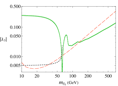
Refer to caption
Figure 1: Values of |λ3||\lambda_{3}| consistent with the relic density data (green solid curve), compared to upper limits on |λ3||\lambda_{3}| from Higgs measurements (black dotted curve) and from null results of DM direct searches (red dashed curve), as discussed in the text.

To determine the λ3\lambda_{3} values that are consistent with the observed relic density, we apply the relevant formulas described above and impose  0.1155≤Ω​h^2≤0.12410.1155\leq\Omega\hat{h}^{2}\leq 0.1241  which is the 90%  confidence level (CL) range of the data  Ω​h^2=0.1198±0.0026\Omega\hat{h}^{2}=0.1198\pm 0.0026  [1]. In Figure 1 we display the result (green solid curve) for  mS3≥10m_{S_{3}}\geq 10 GeV.  It needs to be compared with the red dashed curve, which represents the upper limit on |λ3||\lambda_{3}| inferred from the null result reported by the LUX Collaboration [24]. To arrive at this curve, we used Eq. (36) with  gN​N​h=0.0011g_{NNh}=0.0011,  which is the lower end of its range and thus leads to the loosest limit on |λ3||\lambda_{3}| from the most stringent of DM direct searches to date. For  2​mS3<mh2m_{S_{3}}<m_{h},  the experimental information on the Higgs nonstandard invisible decay implies further restraints. Assuming that the channels  h→S1​S1∗,S2​S2∗h\to S_{1}S_{1}^{*},S_{2}S_{2}^{*}  are absent, we have plotted the black dotted curve upon demanding  ℬ⁡(h→S∗​S)<0.19{\cal B}\bigl(h\to S^{*}S\bigr)<0.19  based on the bounds from the latest analyses of collider data [25]. The opening of the S1,2​S1,2∗S_{1,2}S_{1,2}^{*} channels would cause the dotted curve to shift down.

From the figure, one can infer that the λ3\lambda_{3} contribution to the annihilation rate is much less than half of the required amount if  mS3<90m_{S_{3}}<90 GeV,  except the neighborhood of  mS3=mh/2m_{S_{3}}=m_{h}/2.  In other words, over most of this mass region the λ3\lambda_{3} term in Eq. (30) cannot play the leading role responsible for the observed relic abundance. Therefore, the dominant contribution must come from the effective interactions in Eq. (32), absent other DM candidates. For larger mS3m_{S_{3}}, on the other hand, each of the two sources can generate a nonnegligible effect on the relic density.

IV.2 Effective DM-lepton interactions

The effective operators in Eq. (32) induce DM annihilations into SM leptons and are subject to constraints which may not apply to the Higgs-SkS_{k} renormalizable couplings. From Eq. (33), we derive the amplitudes for the DM annihilation  S3​(p)​S3∗​(p¯)→ℓb−​ℓd+,νb​νdS_{3}(p)\,S_{3}^{*}(\bar{p})\to\ell_{b}^{-}\ell_{d}^{+},\nu_{b}\nu_{d}  to be

ℳS3​S¯3→ℓb​ℓ¯d\displaystyle{\cal M}_{S_{3}\bar{S}_{3}\to\ell_{b}\bar{\ell}_{d}} =\displaystyle\,=\, 1Λ2u¯b[−v2(𝒞b​dL​RPR+𝒞d​bLR∗PL)+γρ(p¯−p)ρ(𝒞b​dLPL+𝒞b​dRPR)]vd,\displaystyle\frac{1}{\Lambda^{2}}\,\bar{u}_{b}\biggl[\frac{-v}{\sqrt{2}}\bigl({\cal C}_{bd}^{\scriptscriptstyle LR}P_{R}+{\cal C}_{db}^{{\scriptscriptstyle LR}*}P_{L}\bigr)\,+\,\gamma^{\rho}(\bar{p}-p)_{\rho\,}\bigl({\cal C}_{bd}^{\scriptscriptstyle L}P_{L}+{\cal C}_{bd}^{\scriptscriptstyle R}P_{R}\bigr)\biggr]v_{d}\;,~~~~
ℳS3​S¯3→νb​νd\displaystyle{\cal M}_{S_{3}\bar{S}_{3}\to\nu_{b}\nu_{d}} =\displaystyle\,=\, 1Λ2​(p¯−p)ρ​u¯b​γρ​(𝒞b​dL​PL−𝒞d​bL​PR)​vd,\displaystyle\frac{1}{\Lambda^{2}}(\bar{p}-p)_{\rho}\,\bar{u}_{b\,}\gamma^{\rho}\bigl({\cal C}_{bd}^{\scriptscriptstyle L}P_{L}-{\cal C}_{db}^{\scriptscriptstyle L}P_{R}\bigr)v_{d}\;, (39)

where ubu_{b} and vdv_{d} are the leptons’ spinors,  PL,R=12​(1∓γ5)P_{L,R}=\frac{1}{2}\bigl(1\mp\gamma_{5}\bigr), 

𝒞b​dϵ=∑k,l𝒰k​3∗𝒰l​3Cb​d​k​lϵ,ϵ=LR,L,R,\displaystyle{\cal C}_{bd}^{\epsilon}\,\,=\,\,\raisebox{3.0pt}{\footnotesize$\displaystyle\sum_{k,l}$}\;{\cal U}_{k3}^{*}\,{\cal U}_{l3}\,C_{bdkl}^{\epsilon}\;,~~~~~~~\epsilon\,\,=\,\,LR,L,R\;, (40)

and for the νb​νd\nu_{b}\nu_{d} channel we have taken into account the neutrinos’ Majorana nature. The contributions of these reactions to the annihilation rate  σann​vrel=a^+b^​vrel2\sigma_{\rm ann}v_{\rm rel}=\hat{a}+\hat{b}v_{\rm rel}^{2}  are

a^\displaystyle\hat{a} =\displaystyle\,=\, 𝒦12​(4​mS32,mℓo2,mℓr2)​v2256​Λ4​π​mS34​[(|𝒞o​rL​R|2+|𝒞r​oL​R|2)​(4​mS32−mℓo2−mℓr2)− 4​Re​(𝒞o​rL​R​𝒞r​oL​R)​mℓo​mℓr],\displaystyle\frac{{\cal K}^{\frac{1}{2}}\bigl(4m_{S_{3}}^{2},m_{\ell_{o}}^{2},m_{\ell_{r}}^{2}\bigr)_{\,}v^{2}}{256\Lambda_{\;\;}^{4}\pi_{\,}m_{S_{3}}^{4}}\Bigl[\bigl(|{\cal C}_{or}^{\scriptscriptstyle LR}|^{2}+|{\cal C}_{ro}^{\scriptscriptstyle LR}|^{2}\bigr)\bigl(4m_{S_{3}}^{2}-m_{\ell_{o}}^{2}-m_{\ell_{r}}^{2}\bigr)\,-\,4\,{\rm Re}\bigl({\cal C}_{or}^{\scriptscriptstyle LR\,}{\cal C}_{ro}^{\scriptscriptstyle LR}\bigr)\,m_{\ell_{o}}m_{\ell_{r}}\Bigr]\,,
b^\displaystyle\hat{b} =\displaystyle\,=\, 𝒦12​(4​mS32,mℓo2,mℓr2)1536​Λ4​π​mS34{(|𝒞o​rL|2+|𝒞o​rR|2)[32mS34−4(mℓo2+mℓr2)mS32−(mℓo2−mℓr2)]2\displaystyle\frac{{\cal K}^{\frac{1}{2}}\bigl(4m_{S_{3}}^{2},m_{\ell_{o}}^{2},m_{\ell_{r}}^{2}\bigr)}{1536\Lambda_{\;\;}^{4}\pi_{\,}m_{S_{3}}^{4}}\Bigl\{\bigl(|{\cal C}_{or}^{\scriptscriptstyle L}|^{2}+|{\cal C}_{or}^{\scriptscriptstyle R}|^{2}\bigr)\Bigl[32m_{S_{3}}^{4}-4\bigl(m_{\ell_{o}}^{2}+m_{\ell_{r}}^{2}\bigr)m_{S_{3}}^{2}-\bigl(m_{\ell_{o}}^{2}-m_{\ell_{r}}^{2}\bigr)\raisebox{1.0pt}{${}^{2}$}\Bigr] (41)
+ 48Re(𝒞o​rL∗𝒞o​rR)mS32mℓomℓr}\displaystyle\hskip 90.41638pt+\;48\,{\rm Re}\bigl({\cal C}_{or}^{{\scriptscriptstyle L}*\,}{\cal C}_{or}^{\scriptscriptstyle R}\bigr)\,m_{S_{3}}^{2}m_{\ell_{o}}m_{\ell_{r}}\Bigr\}
+|𝒞o​rL|2​mS3212​Λ4​π+(𝒞o​r,r​oL​R​terms),\displaystyle\!+\;\frac{|{\cal C}_{or}^{\scriptscriptstyle L}|^{2}m_{S_{3}}^{2}}{12\Lambda_{\;\;}^{4}\pi}\;+\;({\cal C}_{or,ro}^{\scriptscriptstyle LR}\rm~terms)\;,

where  𝒦⁡(x,y,z)=x2+y2+z2−2​(x​y+y​z+x​z){\cal K}(x,y,z)=x^{2}+y^{2}+z^{2}-2(xy+yz+xz)  and summation over  o,r=1,2,3o,r=1,2,3  is implicit, to include all the final lepton states. For  2​mS3>mℓb+mℓd+mh2m_{S_{3}}>m_{\ell_{b}}+m_{\ell_{d}}+m_{h}, the  ϵ=L​R\epsilon=LR  operator also yields  S3​S3∗→ℓb−​ℓd+​hS_{3}S_{3}^{*}\to\ell_{b}^{-}\ell_{d}^{+}h,  but its impact can be neglected in our mS3m_{S_{3}} range of interest.

Since the Δ\Delta’s in Eq. (33) contain many free parameters, to proceed we need to make more specific choices regarding Cb​d​k​lL​R,L,RC_{bdkl}^{\scriptscriptstyle LR,L,R}. For simplicity, we adopt

Cb​d​k​lL​R=2​κL​R​mℓdv​δb​l​δd​k,Cb​d​k​lL=  2​κL​δb​l​δd​k,Cb​d​k​lR=κR​δb​d​δk​l,\displaystyle C_{bdkl}^{\scriptscriptstyle LR}\,\,=\,\,\frac{\sqrt{2}\,\kappa_{LR\,}m_{\ell_{d}}}{v}\,\delta_{bl}\delta_{dk}\;,~~~~~~~C_{bdkl}^{\scriptscriptstyle L}\,\,=\,\,2\kappa_{L}\delta_{bl\,}\delta_{dk}\;,~~~~~~~C_{bdkl}^{\scriptscriptstyle R}\,\,=\,\,\kappa_{R\,}\delta_{bd\,}\delta_{kl}\;, (42)

with κL​R,L,R\kappa_{LR,L,R} being real constants. From Eq. (40) and the unitarity of 𝒰\,\cal U, we then have

𝒞b​dL​R=2​κL​R​mℓdv​𝒰b​3​𝒰d​3∗,𝒞b​dL=  2​κL​𝒰b​3​𝒰d​3∗,𝒞b​dR=κR​δb​d.\displaystyle{\cal C}_{bd}^{\scriptscriptstyle LR}\,\,=\,\,\frac{\sqrt{2}\,\kappa_{LR\,}m_{\ell_{d}}}{v}\;{\cal U}_{b3\,}{\cal U}_{d3}^{*}\;,~~~~~~~{\cal C}_{bd}^{\scriptscriptstyle L}\,\,=\,\,2\kappa_{L}\,{\cal U}_{b3\,}{\cal U}_{d3}^{*}\;,~~~~~~~{\cal C}_{bd}^{\scriptscriptstyle R}\,\,=\,\,\kappa_{R\,}\delta_{bd}\;. (43)

We also need to specify the SkS_{k} masses. Among the different ways to realize 𝖠\sf A in Eq. (15), we concentrate on the least complicated possibility that OO is a real orthogonal matrix, in addition to the right-handed neutrinos being degenerate with  Mν=ℳ​𝟙M_{\nu}={\cal M}\openone,  in which case

𝖠=2​ℳv2​UPMNS​m^ν​UPMNS†.\displaystyle{\sf A}\,\,=\,\,\frac{2_{\,}\cal M}{v^{2}}\,U_{\scriptscriptstyle\rm PMNS\,}\hat{m}_{\nu\,}U_{\scriptscriptstyle\rm PMNS}^{\dagger}\;. (44)

With  𝖠=𝒰​diag​(𝖠^1,𝖠^2,𝖠^3)​𝒰†{\sf A}={\cal U}\,{\rm diag}\bigl(\hat{\mbox{\small$\sf A$}}_{1},\hat{\mbox{\small$\sf A$}}_{2},\hat{\mbox{\small$\sf A$}}_{3}\bigr)\,{\cal U}^{\dagger},  this implies that

𝒰=UPMNS,𝖠^k=2​ℳ​mkv2.\displaystyle{\cal U}\,\,=\,\,U_{\scriptscriptstyle\rm PMNS}\,,~~~~~~~\hat{\mbox{\small$\sf A$}}_{k}\,\,=\,\,\frac{2{\cal M}_{\,}m_{k}}{v^{2}}\,. (45)

The SkS_{k} mass formula in Eq. (31) then becomes

mSk2=μs​02+λs​0​v2+2​(μs​12+λs​1​v2)​ℳ​mkv2+4​(μs​22+λs​2​v2)​ℳ2​mk2v4,\displaystyle m_{S_{k}}^{2}\,=\,\mu_{s0}^{2}+\lambda_{s0}v^{2}\,+\,\frac{2\bigl(\mu_{s1}^{2}+\lambda_{s1}v^{2}\bigr){\cal M}_{\,}m_{k}}{v^{2}}\,+\,\frac{4\bigl(\mu_{s2}^{2}+\lambda_{s2}v^{2}\bigr){\cal M}_{\,}^{2}m_{k}^{2}}{v^{4}}\,, (46)

indicating that the pattern of SkS_{k} masses is connected to the mass hierarchy of the light neutrinos. For definiteness, we pick

μs​02+λs​0​v2=μs​12+λs​1​v2=μs​22+λs​2​v2.\displaystyle\mu_{s0}^{2}+\lambda_{s0}v^{2}\,=\,\mu_{s1}^{2}+\lambda_{s1}v^{2}\,=\,\mu_{s2}^{2}+\lambda_{s2}v^{2}\,. (47)

Thus a normal hierarchy of neutrino masses,  m1<m2≪m3m_{1}<m_{2}\ll m_{3},  would cause S1,2S_{1,2} to be close in mass and lighter than S3S_{3}, implying that at least both S1,2S_{1,2} determine the DM density. As stated earlier, here we examine the simpler scenario with the inverted hierarchy of neutrino masses,  m3≪m1<m2m_{3}\ll m_{1}<m_{2},  so that only S3S_{3} is the DM and the heavier S1,2S_{1,2} have negligible effects on the relic abundance.

For numerical computations below, we need to know the elements of 𝒰\cal U as well as the light neutrino eigenmasses. We employ the central values of the parameter ranges

sin2⁡θ12\displaystyle\sin^{2}\theta_{12} =\displaystyle\,=\, 0.308±0.017,sin2⁡θ23=0.455−0.031+0.139,\displaystyle 0.308\pm 0.017~,~~~~~~~\sin^{2}\theta_{23}~=~0.455_{-0.031}^{+0.139}~,
sin2⁡θ13\displaystyle\sin^{2}\theta_{13} =\displaystyle\,=\, 0.0240−0.0022+0.0019,δ/π=1.31−0.33+0.29,\displaystyle 0.0240_{-0.0022}^{+0.0019}~,\hskip 43.05542pt\delta/\pi~=~1.31_{-0.33}^{+0.29}~,
δ​m2\displaystyle\delta m^{2} =\displaystyle\,=\, m22−m12=(7.54−0.22+0.26)×10−5​eV2,\displaystyle m_{2}^{2}-m_{1}^{2}\,=\,\left(7.54_{-0.22}^{+0.26}\right)\times 10^{-5}\;{\rm eV}^{2}~,
Δ​m2\displaystyle\Delta m^{2} =\displaystyle\,=\, 12​(m12+m22)−m32=(2.38−0.06+0.06)×10−3​eV2\displaystyle\mbox{$\frac{1}{2}$}\bigl(m_{1}^{2}+m_{2}^{2}\bigr)-m_{3}^{2}\,=\,\bigl(2.38_{-0.06}^{+0.06}\bigr)\times 10^{-3}\;{\rm eV}^{2} (48)

from a recent fit to the global data on neutrino oscillation [26] in the case of inverted hierarchy of neutrino masses. Since empirical information on the absolute scale of m1,2,3m_{1,2,3} is still far from precise [1], we set  m3=0m_{3}=0.  Requiring the largest eigenvalue of 𝖠\sf A in Eq. (44) to be unity, we then get  ℳ=6.15×10¹⁴{\cal M}=6.15\times 10^{14} GeV.  Applying these mass numbers and Eq. (47) in Eq. (46) results in  mS1≃1.7​mS3m_{S_{1}}\simeq 1.7_{\,}m_{S_{3}\,} and mS1,S2m_{S_{1},S_{2}} differing by ∼\sim 0.8%.

We can now extract the values of  Λ~≡Λ/|κϵ|1/2\tilde{\Lambda}\equiv\Lambda/|\kappa_{\epsilon}|^{1/2}  that fulfill the relic density requirement using Eq. (41) with the couplings given in Eq. (43). Assuming that only one of κL​R,L,R\kappa_{LR,L,R} is nonzero at a time and that the λ3\lambda_{3} contributions evaluated earlier are absent, we present the results in Figure 2. The curve for  ϵ=L​R\epsilon=LR  arises from a^\hat{a} in Eq. (41), with the contribution from b^\hat{b} having been neglected, whereas the  ϵ=L\epsilon=L or RR  curve comes from b^\hat{b} alone.55 5 The roughly flat behavior of the L​RLR (blue) curve reflects the mS3m_{S_{3}} independence of a^\hat{a} in Eq. (41) for negligible lepton masses and is similar to its counterpart in the quark-flavored-DM scenario [6]. If the λ3\lambda_{3} contributions are also present and nonnegligible, and if they do not cancel the effective-coupling contributions in the  ℓk−​ℓk+\ell_{k}^{-}\ell_{k}^{+}  channels, there will be less room for each of the two sources, which will push the Λ~\tilde{\Lambda} curves upward. On the lower right portion of the plot, we have also drawn an orange area, which satisfies  2​π​Λ~<mS22\pi\tilde{\Lambda}<m_{S_{2}}  for the parameter choices in Eq. (47) and the preceding paragraph. This region corresponds to the parameter space where the effective field theory description is no longer valid [27].

Refer to caption
Figure 2: Values of  Λ~=Λ/|κϵ|1/2\tilde{\Lambda}=\Lambda/|\kappa_{\epsilon}|^{1/2}  for  ϵ=L,R,L​R\epsilon=L,R,LR  which fulfill the relic density constraint, as discussed in the text. In this and the following figures, the (orange) shaded region depicts the parameter space where the effective field theory approach breaks down.

There is another restraint from DM data that should be mentioned. For  mS3<20m_{S_{3}}<20 GeV,  the predicted annihilation rate for the τ+​τ−\tau^{+}\tau^{-} final-state is in some tension with upper limits inferred from searches for DM signals in diffuse gamma-ray data from the Fermi Large Area Telescope observations of dwarf spheroidal satellite galaxies of the Milky Way [28].

More significantly, complementary constraints on the effective lepton-SS couplings are available from experimental studies at LEP  II on the monophoton production process  e+​e−→γ/Ee^{+}e^{-}\to\gamma\,/\penalty\!\!\!\!E  with missing energy  /E/\penalty\!\!\!\!E  in the final state. These measurements were carried out to examine the neutrino counting reaction  e+​e−→γ​ν​ν¯e^{+}e^{-}\to\gamma\nu\bar{\nu}  in the SM and also to look for new particles that are long-lived or stable [29]. Thus the acquired data may be useful for restricting the process  e+​e−→γ​Sk​Sl∗e^{+}e^{-}\to\gamma S_{k}S_{l}^{*}  if Sk,lS_{k,l} are long-lived or, for  k,l≠3k,l\neq 3,  if they decay (sequentially) into S3S_{3} plus light neutrinos. This transition arises from two diagrams each containing an  e+​e−→Sk​Sl∗e^{+}e^{-}\to S_{k}S_{l}^{*}  vertex with the photon being radiated off the e−e^{-} or e+e^{+} line. We have written down its amplitude and sketched the calculation of the cross section, σe​e¯→γ​Sk​S¯l\sigma_{e\bar{e}\to\gamma S_{k}\bar{S}_{l}}, in Appendix  A. Summing it over the final flavors then yields σe​e¯→γ​S​S¯′→γ/E\sigma_{e\bar{e}\to\gamma S\bar{S}^{\prime}\to\gamma\,/\penalty\!\!\!\!E} if Sk,lS_{k,l} are stable or long-lived. If they decay, we can express instead

σe​e¯→γ​S​S¯′→γ/E=∑k,l=13​σe​e¯→γ​Sk​S¯l​ℬk​3​ℬl​3\displaystyle\displaystyle\sigma_{e\bar{e}\to\gamma S\bar{S}^{\prime}\to\gamma\,/\penalty\!\!\!\!E}\,\,=\,\,\raisebox{2.0pt}{\footnotesize$\displaystyle\sum_{k,l\,=1}^{3}$}\,\sigma_{e\bar{e}\to\gamma S_{k}\bar{S}_{l}}\,{\cal B}_{k3}\,{\cal B}_{l3} (49)

with the branching ratios

ℬ13=ℬ⁡(S1→ν​ν′​S3),ℬ23=ℬ⁡(S2→ν​ν′​S3)+ℬ⁡(S2→ν​ν′​S1)​ℬ13,ℬ33= 1,\displaystyle{\cal B}_{13}\,=\,{\cal B}(S_{1}\to\nu\nu^{\prime}S_{3})\;,\hskip 17.22217pt{\cal B}_{23}\,=\,{\cal B}(S_{2}\to\nu\nu^{\prime}S_{3})+{\cal B}(S_{2}\to\nu\nu^{\prime}S_{1})\,{\cal B}_{13}\;,\hskip 17.22217pt{\cal B}_{33}\,=\,1\;,~~~ (50)

where the sum includes only kinematically allowed channels and  ℬ⁡(Sl→ν​ν′​Sk)=ΓSl→ν​ν′​Sk/ΓSl{\cal B}(S_{l}\to\nu\nu^{\prime}S_{k})=\Gamma_{S_{l}\to\nu\nu^{\prime}S_{k}}/\Gamma_{S_{l}}  from the rates derived in Appendix  B.

The LEP  II experiments on  e+​e−→γ/Ee^{+}e^{-}\to\gamma\,/\penalty\!\!\!\!E  had c.m. energies within the range  130-207  GeV,  and the observed cross-sections vary also with cuts on the photon energy EγE_{\gamma} and angle θγ\theta_{\gamma} relative to the beam direction. From a collection of these data [29] tabulated in Ref. [30], one can see that the majority of the measured and SM values of the cross section agree with each other at the one-sigma level. Consequently, to bound the  e​e​S​S′eeSS^{\prime}  couplings, we may require σe​e¯→γ​S​S¯′→γ/E\sigma_{e\bar{e}\to\gamma S\bar{S}^{\prime}\to\gamma\,/\penalty\!\!\!\!E} not to exceed the corresponding one-sigma empirical errors (after combining the statistical and systematic errors in quadrature).

Applying this condition and assuming as before that only one of the CC couplings in Eq. (33) is nonzero at a time, for the coupling choices in Eq. (42) we find that κL​R/Λ2\kappa_{LR}/\Lambda^{2} does not get any meaningful limitations from the LEP  II measurements, which is not unexpected because the resulting e​e​S​S′eeSS^{\prime} interaction is suppressed by the electron mass, as Eq. (62) indicates. On the other hand, they do translate into moderate restraints on κL⁡(R)/Λ2\kappa_{L(R)}/\Lambda^{2}. More precisely, from the data, we infer the dotted curves shown in Figure  3 which represent lower limits on Λ~\tilde{\Lambda} and therefore reduce the parameter space consistent with the observed relic abundance (the solid thin bands), so that now  mS3​ ≲ ​24​(43)m_{S_{3}}\mbox{\footnotesize\;$\lesssim$\;}24\,(43)  GeV  is excluded for  ϵ=L⁡(R)\epsilon=L\,(R).  It is clear from this simple exercise that future e+​e−e^{+}e^{-} machines with greater energies and luminosities, such as the International Linear Collider  [31], can be expected to probe more stringently this new-physics scenario, if they detect no signals beyond the SM.

Refer to caption
Figure 3: Values of  Λ~=Λ/|κϵ|1/2\tilde{\Lambda}=\Lambda/|\kappa_{\epsilon}|^{1/2}  for  ϵ=L\epsilon=L and RR  which are compatible with the observed relic abundance (solid thin bands), compared to lower limits on Λ~\tilde{\Lambda} inferred from measurements of  e+​e−→γ/Ee^{+}e^{-}\to\gamma\,/\penalty\!\!\!\!E  at LEP  II (dotted curves).

Another important implication of the dimension-6 effective  ℓ​ℓ′​S​S′\ell\ell^{\prime}SS^{\prime}  interactions is that they can give rise to the flavor-changing decay  ℓa−→ℓb−​ℓc−​ℓd+\ell_{a}^{-}\to\ell_{b}^{-}\ell_{c}^{-}\ell_{d}^{+}  via one-loop diagrams involving internal Sk,lS_{k,l} if at least one of the couplings is flavor violating. Such decays have been searched for over the years, but with null results so far, leading to increasingly severe bounds on their branching ratios [1]. Consequently, their data may give rise to substantial restrictions on the couplings.

We again assume that only one of the couplings in Eq. (33) is contributing at a time. Since CRC^{\scriptscriptstyle R} conserves flavor, only CL​RC^{\scriptscriptstyle LR} and CLC^{\scriptscriptstyle L} as specified in Eq. (42) are pertinent. Thus we can express the amplitudes for  ℓa−→ℓb−​ℓc−​ℓd+\ell_{a}^{-}\to\ell_{b}^{-}\ell_{c}^{-}\ell_{d}^{+}  in each case as

ℳℓa→ℓb​ℓc​ℓ¯dL​R\displaystyle{\cal M}_{\ell_{a}\to\ell_{b}\ell_{c}\bar{\ell}_{d}}^{\scriptscriptstyle LR} =\displaystyle=\, ℐ⁡(mSk,mSl)​v216​π2​Λ4𝒰p​k∗𝒰s​k𝒰q​l𝒰r​l∗[u¯c(Cc​a​p​qL​RPR+Ca​c​q​pLR∗PL)uau¯b(Cb​d​r​sL​RPR+Cd​b​s​rLR∗PL)vd\displaystyle\frac{{\cal I}\bigl(m_{S_{k}},m_{S_{l}}\bigr)v^{2}}{16_{\;}\!\pi_{\,\,}^{2}\Lambda^{4}}\,{\cal U}_{pk\,}^{*}{\cal U}_{sk\,}{\cal U}_{ql\,}{\cal U}_{rl}^{*}\bigl[\bar{u}_{c}\bigl(C_{capq}^{\scriptscriptstyle LR}P_{R}+C_{acqp}^{{\scriptscriptstyle LR}*}P_{L}\bigr)u_{a\,}\bar{u}_{b}\bigl(C_{bdrs}^{\scriptscriptstyle LR}P_{R}+C_{dbsr}^{{\scriptscriptstyle LR}*}P_{L}\bigr)v_{d} (51)
−(b↔c)],\displaystyle\hskip 129.16626pt-\;(b\leftrightarrow c)\bigr]\,,
ℳℓa→ℓb​ℓc​ℓ¯dL\displaystyle{\cal M}_{\ell_{a}\to\ell_{b}\ell_{c}\bar{\ell}_{d}}^{\scriptscriptstyle L} =\displaystyle=\, 𝒥⁡(mSk,mSl)8​π2​Λ4​𝒰p​k∗​𝒰r​k​𝒰q​l​𝒰s​l∗​(Cc​a​p​qL​Cb​d​s​rL+Cb​a​p​qL​Cc​d​s​rL)​u¯c​γρ​PL​ua​u¯b​γρ​PL​vd,\displaystyle\frac{{\cal J}\bigl(m_{S_{k}},m_{S_{l}}\bigr)}{8_{\;}\!\pi_{\,\,}^{2}\Lambda^{4}}\,{\cal U}_{pk\,}^{*}{\cal U}_{rk}\,{\cal U}_{ql\,}{\cal U}_{sl}^{*}\,\bigl(C_{capq\,}^{\scriptscriptstyle L}C_{bdsr}^{\scriptscriptstyle L}+C_{bapq\,}^{\scriptscriptstyle L}C_{cdsr}^{\scriptscriptstyle L}\bigr)\bar{u}_{c}\gamma^{\rho}P_{L}u_{a}\,\bar{u}_{b}\gamma_{\rho}P_{L}v_{d}\;, (52)

where  k,l,p,q,r,s=1,2,3k,l,p,q,r,s=1,2,3  are summed over and ℐ\cal I and 𝒥\cal J are loop functions. With the choices of CL​R,LC^{\scriptscriptstyle LR,L} in Eq. (42), we arrive at

ℐ⁡(m,n)=m2​ln⁡(n/m)m2−n2,𝒥⁡(m,n)=m2​(ln⁡Λn+14)+m4​ln⁡(n/m)m2−n2,\displaystyle{\cal I}(m,n)\,\,=\,\,\frac{m^{2}\ln(n/m)}{m^{2}-n^{2}}~,~~~~~~~{\cal J}(m,n)\,\,=\,\,m^{2}\biggl(\ln\frac{\Lambda}{n}+\frac{1}{4}\biggr)\,+\,\frac{m^{4}\ln(n/m)}{m^{2}-n^{2}}~, (53)

where we have dropped terms that vanished after kk is summed over in Eqs.  (51) and (52) due to  a≠b,c,da\neq b,c,d  and the unitarity of 𝒰\,\cal U. We have also taken the cutoff in the loop integration to be the same as the scale Λ\Lambda and neglected the momenta of the external particles.

Upon comparing the resulting branching ratio of  ℓa−→ℓb−​ℓc−​ℓd+\ell_{a}^{-}\to\ell_{b}^{-}\ell_{c}^{-}\ell_{d}^{+}  to its measured bound, one can then derive a limit on  Λ/|κL​R|1/2\Lambda/|\kappa_{LR}|^{1/2},  assuming that only CL​RC^{\scriptscriptstyle LR} is nonzero. The relevant modes are  μ−→e−​e−​e+\mu^{-}\to e^{-}e^{-}e^{+}  and  τ−→e−​e−​e+,μ−​μ−​μ+,e−​e−​μ+,μ−​μ−​e+,μ−​e−​e+,e−​μ−​μ+\tau^{-}\to e^{-}e^{-}e^{+},\mu^{-}\mu^{-}\mu^{+},e^{-}e^{-}\mu^{+},\mu^{-}\mu^{-}e^{+},\mu^{-}e^{-}e^{+},e^{-}\mu^{-}\mu^{+},  for which only experimental bounds on the branching ratios are available. Although the strictest among them is  ℬ(μ−→e−e−e+)<exp1.0×10−12{\cal B}\bigl(\mu^{-}\to e^{-}e^{-}e^{+}\bigr){}_{\rm exp}<1.0\times 10^{-12},  we find that  ℬ(τ−→μ−μ−μ+)<exp2.1×10−8{\cal B}\bigl(\tau^{-}\to\mu^{-}\mu^{-}\mu^{+}\bigr){}_{\rm exp}<2.1\times 10^{-8}  [1] yields the strongest constraint, namely

Λ|κL​R|1/2>  11​GeV,\displaystyle\frac{\Lambda}{|\kappa_{LR}|^{1/2}}\,\,>\,\,11\rm~GeV\,, (54)

which is consistent with the L​RLR curve in Figure  2. This is mainly due to the enhancement from the lepton mass factor in the rate of  τ−→μ−​μ−​μ+\tau^{-}\to\mu^{-}\mu^{-}\mu^{+},  as can be seen from the expressions for  ℓ′⁣−→ℓ−​ℓ−​ℓ+\ell^{\prime-}\to\ell^{-}\ell^{-}\ell^{+}  rates collected in Appendix  C.

Refer to caption
Figure 4: Values of Λ\Lambda for CLC^{\scriptscriptstyle L} in Eq. (42) with  κL=1\kappa_{L}=1  which fulfill the relic density constraint (green thin band), compared to the lower limits on Λ\Lambda from the LEP  II data on  e+​e−→γ/Ee^{+}e^{-}\to\gamma\,/\penalty\!\!\!\!E  (green dotted curve) and from searches for  μ−→e−​e−​e+\mu^{-}\to e^{-}e^{-}e^{+}  (red solid curve) and  τ−→μ−​μ−​e+\tau^{-}\to\mu^{-}\mu^{-}e^{+}  (red dashed curve).

If instead only CLC^{\scriptscriptstyle L} in Eq. (42) is present, ℬ(μ−→e−e−e+)exp{\cal B}\bigl(\mu^{-}\to e^{-}e^{-}e^{+}\bigr){}_{\rm exp} turns out to impose the most stringent constraint among these decays in the  mS3​ ≳ ​50m_{S_{3}}\mbox{\footnotesize\;$\gtrsim$\;}50 GeV  region, whereas for lower masses  ℬ(τ−→μ−μ−e+)<exp1.7×10−8{\cal B}\bigl(\tau^{-}\to\mu^{-}\mu^{-}e^{+}\bigr){}_{\rm exp}<1.7\times 10^{-8}  [1] is the most restrictive. The formulas for their rates are also listed in Appendix  C. In Figure 4 we depict the resulting lower-limits on Λ\Lambda. In this case, we set  κL=1\kappa_{L}=1  due to the ln​Λ{\rm ln}\Lambda dependence of the  μ−→e−​e−​e+\mu^{-}\to e^{-}e^{-}e^{+}  rate. The plot reveals that above  mS3∼500m_{S_{3}}\sim 500 GeV  the Λ\Lambda values consistent with the observed relic density are in conflict with the bound from the  μ−→e−​e−​e+\mu^{-}\to e^{-}e^{-}e^{+}  data. This significantly shrinks the allowed parameter space already decreased by the restraint from the LEP  II measurements.

IV.3 Flavor-violating Higgs decay

The recently discovered Higgs boson can potentially offer a window into physics beyond the SM. The presence of new particles can bring about modifications to the standard decay modes of the Higgs and/or cause it to undergo exotic decays [32]. As data from the LHC continues to accumulate with increasing precision, they may uncover clues of new physics in the Higgs couplings.

The CMS Collaboration [33] has recently reported the detection of a slight excess of  h→μ±​τ∓h\to\mu^{\pm}\tau^{\mp}  events with a significance of 2.5σ\sigma. If interpreted as a signal, the result corresponds to a branching fraction of  ℬ⁡(h→μ​τ)=ℬ⁡(h→μ−​τ+)+ℬ⁡(h→μ+​τ−)=(0.89−0.37+0.40){\cal B}(h\to\mu\tau)={\cal B}(h\to\mu^{-}\tau^{+})+{\cal B}(h\to\mu^{+}\tau^{-})=\bigl(0.89^{+0.40}_{-0.37}\bigr)%,  but as a statistical fluctuation it translates into a limit of  ℬ⁡(h→μ​τ)<1.57{\cal B}(h\to\mu\tau)<1.57%  at 95% CL [33]. It is too early to draw a definite conclusion from this finding, but it would constitute clear evidence of physics beyond the SM if substantiated by future measurements. Assuming that the tentative signal hint is true, we investigate whether the SkS_{k} interactions could effect such an exotic Higgs decay within the allowed parameter space.66 6 The CMS excess has also been addressed in the contexts of other new-physics scenarios [34].

One can write the amplitude for  h→ℓb−​ℓd+h\to\ell_{b}^{-}\ell_{d}^{+}  as

ℳh→ℓb​ℓ¯d=yb​dSM+yb​dnewv​u¯b​(mℓb​PL+mℓd​PR)​vd,\displaystyle{\cal M}_{h\to\ell_{b}\bar{\ell}_{d}}\,\,=\,\,\frac{y_{bd}^{\scriptscriptstyle\rm SM}+y_{bd}^{\rm new}}{v}\,\bar{u}_{b}\bigl(m_{\ell_{b}}P_{L}+m_{\ell_{d}}P_{R}\bigr)v_{d}\;, (55)

corresponding to the rate

Γh→ℓb​ℓ¯d=mh|yb​dSM+yb​dnew|216​π​v2​(mℓb2+mℓd2),\displaystyle\Gamma_{h\to\ell_{b}\bar{\ell}_{d}}\,\,=\,\,\frac{m_{h\,}\bigl|y_{bd}^{\scriptscriptstyle\rm SM}+y_{bd}^{\rm new}\bigr|\raisebox{1.0pt}{${}^{2}$}}{16\pi v^{2}}\bigl(m_{\ell_{b}}^{2}+m_{\ell_{d}}^{2}\bigr)\;, (56)

where  yb​dSM=δb​dy_{bd}^{\scriptscriptstyle\rm SM}=\delta_{bd}  in the SM at tree level and yb​dnewy_{bd}^{\rm new} stands for the new contribution. The main contribution to yb​dnewy_{bd}^{\rm new} originates from a one-loop diagram involving internal SkS_{k}, one h​Sk​SkhS_{k}S_{k} vertex from the renormalizable Lagrangian in Eq. (30), and one Sk​Sk​ℓ​ℓ′S_{k}S_{k}\ell\ell^{\prime} vertex from a dimension-six operator in Eq. (32). It turns out that for the latter coupling only OL​RO^{\scriptscriptstyle LR} matters, as the loop contributions of OL,RO^{\scriptscriptstyle L,R} vanish. Thus, focusing on the case in which  mh<2​mSkm_{h}<2m_{S_{k}}  and CL​RC^{\scriptscriptstyle LR} is given by Eq. (42), we obtain

yb​dnew=κL​R​λk​𝒰d​k∗​𝒰b​k​v216​π2​Λ2​(ln⁡Λ2mSk2+1−2​4​mSk2mh2−1​sin−1⁡mh2​mSk),\displaystyle y_{bd}^{\rm new}\,\,=\,\,\frac{\kappa_{LR\,}\lambda_{k}\,{\cal U}_{dk\,}^{*}{\cal U}_{bk\,}v^{2}}{16\pi_{\,\,}^{2}\Lambda^{2}}\left(\ln\frac{\Lambda^{2}}{m_{S_{k}}^{2}}+1-2\sqrt{\frac{4m_{S_{k}}^{2}}{m_{h}^{2}}-1}\;\sin^{-1}\frac{m_{h}}{2m_{S_{k}}}\right), (57)

where summation over  k=1,2,3k=1,2,3  is implicit and we have again taken the cutoff in the loop integration to be the same as Λ\Lambda. The Sk​Sk​ℓ​ℓ′S_{k}S_{k}\ell\ell^{\prime} coupling alone can generate one-loop contributions to the off-diagonal elements of the charged-lepton mass matrix, but we estimate their impact on its eigenvalues to be small. Therefore, yb​dnewy_{bd}^{\rm new} in Eq. (57) is largely unaffected as the leading contribution of SkS_{k} to  h→ℓb−​ℓd+h\to\ell_{b}^{-}\ell_{d}^{+}. 

Since  h→τ+​τ−,μ+​μ−h\to\tau^{+}\tau^{-},\mu^{+}\mu^{-}  also receive the SkS_{k} contributions in Eq. (57), we need to take into account the relevant data. The ATLAS and CMS Collaborations have reported the observations of  h→τ+​τ−h\to\tau^{+}\tau^{-}  and measured its signal strength to be  σ/σSM=1.42−0.38+0.44\sigma/\sigma_{\scriptscriptstyle\rm SM}=1.42^{+0.44}_{-0.38} and 0.91±0.270.91\pm 0.27,  respectively [22, 35]. In contrast, the only experimental information on  h→μ+​μ−h\to\mu^{+}\mu^{-}  are the bounds  ℬ⁡(h→μ​μ¯)<1.5×10⁻³{\cal B}(h\to\mu\bar{\mu})<1.5\times 10^{-3} and 1.6×10−31.6\times 10^{-3}  from ATLAS and CMS, respectively [36, 37]. In view of these data, we demand the SkS_{k} contributions to respect

0.7<Γh→τ​τ¯Γh→τ​τ¯SM<  1.8,Γh→μ​μ¯Γh→μ​μ¯SM<  6.7,\displaystyle 0.7\,\,<\,\,\frac{\Gamma_{h\to\tau\bar{\tau}}}{\Gamma_{h\to\tau\bar{\tau}}^{\scriptscriptstyle\rm SM}}\,\,<\,\,1.8~,~~~~~~~\frac{\Gamma_{h\to\mu\bar{\mu}}}{\Gamma_{h\to\mu\bar{\mu}}^{\scriptscriptstyle\rm SM}}\,\,<\,\,6.7~, (58)

where  Γh→τ​τ¯SM=257\Gamma_{h\to\tau\bar{\tau}}^{\scriptscriptstyle\rm SM}=257 keV  and  Γh→μ​μ¯SM=894\Gamma_{h\to\mu\bar{\mu}}^{\scriptscriptstyle\rm SM}=894 eV  [23] for  mh=125.1m_{h}=125.1 GeV. 

Due to the lnΛ\Lambda dependence of yb​dnewy_{bd}^{\rm new}, we also set  κL​R=1\kappa_{LR}=1.  It follows that, for illustration, we can select  (mS3,Λ)=(70,79)\bigl(m_{S_{3}},\Lambda\bigr)=(70,79) and (200,78)  GeV  from the L​RLR (blue) curve in Figure 2, implying that we have assumed λ3\lambda_{3} to be negligible. Choosing also  λ1=λ2\lambda_{1}=\lambda_{2}  for simplification, we find that for  (mS3,Λ)=(70,79)\bigl(m_{S_{3}},\Lambda\bigr)=(70,79) GeV  the SkS_{k} contributions lead to  0.0026>|yμ​τ,τ​μnew|​mτ/v>0.00210.0026>\bigl|y_{\mu\tau,\tau\mu}^{\rm new}\bigr|m_{\tau}/v>0.0021,  or  0.79%>ℬ⁡(h→μ​τ)>0.52%0.79\%>{\cal B}(h\to\mu\tau)>0.52\%,  compatible with the range of the CMS finding on the potential signal [33], if  −7.2<λ1<−5.8-7.2<\lambda_{1}<-5.8.  For  (mS3,Λ)=(200,78)\bigl(m_{S_{3}},\Lambda\bigr)=(200,78) GeV,  we obtain the same ℬ⁡(h→μ​τ){\cal B}(h\to\mu\tau) range if  −2.9<λ1<−2.4-2.9<\lambda_{1}<-2.4.  All these numbers correspond to  1.6<Γh→τ​τ¯/Γh→τ​τ¯SM<1.81.6<\Gamma_{h\to\tau\bar{\tau}}/\Gamma_{h\to\tau\bar{\tau}}^{\scriptscriptstyle\rm SM}<1.8  and  1.8<Γh→μ​μ¯/Γh→μ​μ¯SM<2.01.8<\Gamma_{h\to\mu\bar{\mu}}/\Gamma_{h\to\mu\bar{\mu}}^{\scriptscriptstyle\rm SM}<2.0,  which conform to the conditions in Eq. (58) and are therefore testable soon with forthcoming data from the LHC. Moreover, we determine that  Γh→e​τ=0.053​Γh→μ​τ\Gamma_{h\to e\tau}=0.053_{\,}\Gamma_{h\to\mu\tau}.  Although the preferred values of  |λ1,2||\lambda_{1,2}|  seem to be sizable, they are still below the perturbativity limit of 4​π4\pi mentioned earlier. It is worth noting that the  |yμ​τ,τ​μnew|​mτ/v\bigl|y_{\mu\tau,\tau\mu}^{\rm new}\bigr|m_{\tau}/v  numbers above are below the upper limit of 0.016 inferred from the measured bound on the  τ→μ​γ\tau\to\mu\gamma  decay [38].

We have seen from the limited exercises performed in this paper that the MFV framework offers a systematic way to explore potential relations between DM, neutrinos, and the Higgs boson through a variety of processes which can be checked experimentally. More sophisticated choices of the coefficients CL,R,L​RC^{\scriptscriptstyle L,R,LR} than those in Eq. (42) would then allow the examination of a greater number of leptonic observables.

V Conclusions

We have considered DM which is a singlet under the SM gauge group and a member of a scalar triplet under the lepton flavor group. The triplet is odd under an extra Z2Z_{2} symmetry which renders the DM candidate stable. We apply the MFV principle to all the lepton-flavored particles in the theory which includes three right-handed neutrinos taking part in the seesaw mechanism for neutrino mass generation. The new scalars couple to SM particles via Higgs-portal renormalizable interactions and dimension-six operators involving leptons. The MFV framework allows us to make interesting phenomenological connections between the DM, Higgs, and lepton sectors. We examine restrictions on the new scalars from the Higgs boson data, observed relic density, DM  direct searches, LEP  II measurements on e+​e−e^{+}e^{-} scattering into a photon plus missing energy, and experimental bounds on flavor-violating lepton decays. We obtain viable parameter space that can be probed further by future experiments. Our simple choices of the new scalars’ effective couplings illustrate how various data can constrain them in complementary ways. We also explore whether the scalar interactions can account for the tentative hint of the Higgs flavor-violating decay  h→μ​τh\to\mu\tau  recently detected in the CMS experiment. Their contributions, occurring at the one-loop level, can give rise to a decay rate compatible with the CMS finding and at the same time fulfill requirements from other Higgs data. If it is not confirmed by upcoming measurements, the acquired data will place stronger limitations on the considered scenario of lepton-flavored DM with MFV. Last but not least, it is clear from our analysis that next-generation e+​e−e^{+}e^{-} machines with high energies and luminosities, such as the International Linear Collider, have considerable potential for testing different aspects of this kind of new physics in greater detail.

Acknowledgements.
We would like to thank Xiao-Gang He for helpful comments. We also thank Brian Batell for remarks concerning the stability of lepton-flavored dark matter. This work was supported in part by the MOE Academic Excellence Program (Grant No. 102R891505) and the NCTS.

Appendix A Cross section of 𝒆+​𝒆−→𝜸​𝑺𝒌​𝑺𝒍∗\bm{e^{+}e^{-}\to\gamma S_{k}S_{l}^{*}}

For the scattering  e−​(p)​e+​(p¯)→γ⁡(k)​Sk​(q)​Sl∗​(q¯)e^{-}(p)\,e^{+}(\bar{p})\to\gamma(\textsc{k})\,S_{k}(q)\,S_{l}^{*}(\bar{q}),  we define the Lorentz-invariant kinematical variables

s\displaystyle s =\displaystyle\,=\, (p+p¯)2,s′=(q+q¯)2,t=(p¯−q¯)2,t′=(p−q)2,\displaystyle(p+\bar{p})^{2}\,,\hskip 30.1388pts^{\prime}\,\,=\,\,(q+\bar{q})^{2}\,,\hskip 30.1388ptt\,\,=\,\,(\bar{p}-\bar{q})^{2}\,,\hskip 30.1388pt\!t^{\prime}\,\,=\,\,(p-q)^{2}\,,
u\displaystyle u =\displaystyle\,=\, (p¯−q)2,u′=(p−q¯)2,w=  2​k⋅p,w¯=  2​k⋅p¯.\displaystyle(\bar{p}-q)^{2}\,,\hskip 30.1388ptu^{\prime}\,\,=\,\,(p-\bar{q})^{2}\,,\hskip 25.83325ptw\,\,=\,\,2_{\,}\textsc{k}\cdot p\,,\hskip 34.44434pt\bar{w}\,\,=\,\,2_{\,}\textsc{k}\cdot\bar{p}\,.~~~ (59)

We derive its amplitude ℳe​e¯→γ​Sk​S¯l{\cal M}_{e\bar{e}\to\gamma S_{k}\bar{S}_{l}} from two diagrams each with an  e−​e+→Sk​Sl∗e^{-}e^{+}\to S_{k}S_{l}^{*}  vertex and the photon radiated from the e−e^{-} or e+e^{+} leg. Thus, in the limit of massless e±e^{\pm},

ℳe​e¯→γ​Sk​S¯l\displaystyle{\cal M}_{e\bar{e}\to\gamma S_{k}\bar{S}_{l}} =\displaystyle= 4​α​πΛ2v¯e¯[(/q¯−/q)(ck​lLPL+ck​lRPR)−v2(ck​lL​RPR+c¯k​lL​RPL)]/p−/kw/ε∗ue\displaystyle\frac{\sqrt{4\alpha_{\;\!}\pi}}{\Lambda^{2}}\,\bar{v}_{\bar{e}}\bigg[(/\penalty{\!\!\!\bar{q}}-/\penalty{\!\!\!q})\bigl(\textsc{c}_{kl}^{\scriptscriptstyle L}P_{L}+\textsc{c}_{kl}^{\scriptscriptstyle R}P_{R}\bigr)-\frac{v}{\sqrt{2}}\bigl(\textsc{c}_{kl}^{\scriptscriptstyle LR}P_{R}+\bar{\textsc{c}}_{kl}^{\scriptscriptstyle LR}P_{L}\bigr)\bigg]\frac{/\penalty{\!\!\!p}-/\penalty{\!\!\!\textsc{k}}}{w}\,/\penalty{\!\!\!\varepsilon}^{*}u_{e} (60)
−4​α​πΛ2v¯e¯/ε∗/p¯−/kw¯[(/q¯−/q)(ck​lLPL+ck​lRPR)−v2(ck​lL​RPR+c¯k​lL​RPL)]ue,\displaystyle\!\!\!-\;\frac{\sqrt{4\alpha_{\;\!}\pi}}{\Lambda^{2}}\,\bar{v}_{\bar{e}}\,/\penalty{\!\!\!\varepsilon}^{*}\,\frac{/\penalty{\!\!\!\bar{p}}-/\penalty{\!\!\!\textsc{k}}}{\bar{w}}\bigg[(/\penalty{\!\!\!\bar{q}}-/\penalty{\!\!\!q})\bigl(\textsc{c}_{kl}^{\scriptscriptstyle L}P_{L}+\textsc{c}_{kl}^{\scriptscriptstyle R}P_{R}\bigr)-\frac{v}{\sqrt{2}}\bigl(\textsc{c}_{kl}^{\scriptscriptstyle LR}P_{R}+\bar{\textsc{c}}_{kl}^{\scriptscriptstyle LR}P_{L}\bigr)\bigg]u_{e}\;,~~~~~~~

where  α=1/128\alpha=1/128  is the fine-structure constant,

ck​lϵ=∑n,o𝒰k​n†𝒰o​lC11​n​oϵ,ϵ=L,R,LR,c¯k​lL​R=(cl​kL​R)∗.\displaystyle\textsc{c}_{kl}^{\epsilon}\,\,=\,\,\raisebox{3.0pt}{\footnotesize$\displaystyle\sum_{n,o}$}\;{\cal U}_{kn}^{\dagger}\,{\cal U}_{ol}\,C_{11no}^{\epsilon}\;,~~~~~\epsilon\,\,=\,\,L,R,LR\;,~~~~~~~\bar{\textsc{c}}_{kl}^{\scriptscriptstyle LR}\,\,=\,\,\bigl(\textsc{c}_{lk}^{\scriptscriptstyle LR}\bigr)^{*}\,. (61)

Hence for the choices in Eq. (42)

ck​lL=  2​κL​𝒰1​k∗​𝒰1​l,ck​lR=κR​δk​l,ck​lL​R=2​κL​R​mev​𝒰1​k∗​𝒰1​l.\displaystyle\textsc{c}_{kl}^{\scriptscriptstyle L}\,\,=\,\,2\kappa_{L}\,{\cal U}_{1k\,}^{*}{\cal U}_{1l}\;,~~~~~~~\textsc{c}_{kl}^{\scriptscriptstyle R}\,\,=\,\,\kappa_{R\,}\delta_{kl}\;,~~~~~~~\textsc{c}_{kl}^{\scriptscriptstyle LR}\,\,=\,\,\frac{\sqrt{2}\,\kappa_{LR\,}m_{e}}{v}\;{\cal U}_{1k\,}^{*}{\cal U}_{1l}\;. (62)

It is easy to check that  ℳe​e¯→γ​Sk​S¯l{\cal M}_{e\bar{e}\to\gamma S_{k}\bar{S}_{l}}  respects electromagnetic gauge invariance. Averaging (summing) its absolute square over the initial (final) spins, one then obtains

|ℳe​e¯→γ​Sk​S¯l|2¯\displaystyle\overline{\big|{\cal M}_{e\bar{e}\to\gamma S_{k}\bar{S}_{l}}\big|\raisebox{1.0pt}{${}^{2}$}} =\displaystyle= 2​α​π​(|ck​lL|2+|ck​lR|2)Λ4​w​w¯{2(mSk2−mSl2)[mSk2s−mSl2s+(t−u)w−(t′−u′)w¯]\displaystyle\frac{2\alpha_{\;\!}\pi_{\;\!}\big(|\textsc{c}_{kl}^{\scriptscriptstyle L}|^{2}+|\textsc{c}_{kl}^{\scriptscriptstyle R}|^{2}\big)}{\Lambda^{4\,}w_{\;\!}\bar{w}}\Big\{2\Big(m_{S_{k}}^{2}-m_{S_{l}}^{2}\Big)\Big[m_{S_{k}}^{2}s-m_{S_{l}}^{2}s+(t-u)w-\big(t^{\prime}-u^{\prime}\big)\bar{w}\Big] (63)
+(w2+w¯2+2ss′)(s′−2mSk2−2mSl2)−s′(t−u)2−s′(t′−u′)}2\displaystyle\hskip 50.00008pt+\,\bigl(w^{2}+\bar{w}^{2}+2ss^{\prime}\big)\Big(s^{\prime}-2m_{S_{k}}^{2}-2m_{S_{l}}^{2}\Big)-s^{\prime}(t-u)^{2}-s^{\prime}\big(t^{\prime}-u^{\prime}\big)\raisebox{1.0pt}{${}^{2}$}\Big\}
+α​π​v2Λ4​w​w¯​(|ck​lL​R|2+|cl​kL​R|2)​(s2+s′2).\displaystyle+\;\frac{\alpha_{\;\!}\pi_{\;\!}v^{2}}{\Lambda^{4\,}w_{\;\!}\bar{w}}\bigl(|\textsc{c}_{kl}^{\scriptscriptstyle LR}|^{2}+|\textsc{c}_{lk}^{\scriptscriptstyle LR}|^{2}\bigr)\bigl(s^{2}+s^{\prime 2}\bigr)\,.

This leads to the cross section

σe​e¯→γ​Sk​S¯l=∫Eγ​d​Eγ​d​(cos⁡θγ)​d​Ω¯S2​(4​π)4​s​1−2​mSk2+2​mSl2s−2​Eγ​s+(mSk2−mSl2s−2​Eγ​s)2​|ℳe​e¯→γ​Sk​S¯l|2¯,\displaystyle\sigma_{e\bar{e}\to\gamma S_{k}\bar{S}_{l}}=\int\frac{E_{\gamma}\,dE_{\gamma}\,d(\cos\theta_{\gamma})\,d\bar{\Omega}_{S}}{2(4\pi)^{4}\,s}\sqrt{1-\frac{2m_{S_{k}}^{2}+2m_{S_{l}}^{2}}{s-2E_{\gamma}\sqrt{s}}+\Biggl(\frac{m_{S_{k}}^{2}-m_{S_{l}}^{2}}{s-2E_{\gamma}\sqrt{s}}\Biggr)\raisebox{12.0pt}{${}^{\!\!\!2}$}}~\overline{|{\cal M}_{e\bar{e}\to\gamma S_{k}\bar{S}_{l}}|^{2}}\;,~~~~ (64)

where EγE_{\gamma} and θγ\theta_{\gamma} are the photon energy and angle with respect to the e−e^{-} or e+e^{+} beam direction in the c.m. frame of the e+​e−e^{+}e^{-} pair, Ω¯S\bar{\Omega}_{S} denotes the solid angle of either SkS_{k} or Sl∗S_{l}^{*} in the c.m. frame of the Sk​Sl∗S_{k}S_{l}^{*} pair. The photon energy range is

Eγmin≤Eγ≤Eγmax=s−(mSk+mSl)22​s,\displaystyle E_{\gamma}^{\rm min}\,\,\leq\,\,E_{\gamma}\,\,\leq\,\,E_{\gamma}^{\rm max}\,\,=\,\,\frac{s-(m_{S_{k}}+m_{S_{l}})^{2}}{2\sqrt{s}}\;, (65)

where EγminE_{\gamma}^{\rm min} is an experimental cut. In the numerical evaluation of the integral, the θγ\theta_{\gamma} range is also subject to cuts.

It is worth mentioning that one could alternatively estimate  σe​e¯→γ​Sk​S¯l\sigma_{e\bar{e}\to\gamma S_{k}\bar{S}_{l}}  in the so-called radiator approximation [39]. It is given by

σe​e¯→γ​Sk​S¯l=∫d​cγ​d​xγ​ℋ​(cγ,xγ,s)​σ^​(s^),\displaystyle\displaystyle\sigma_{e\bar{e}\to\gamma S_{k}\bar{S}_{l}}\,\,=\,\,\int dc_{\gamma}\,dx_{\gamma}\,{\cal H}\big(c_{\gamma},x_{\gamma};s\big)\,\hat{\sigma}(\hat{s})\,, (66)
cγ=cos⁡θγ,xγ=2​Eγs,ℋ⁡(cγ,xγ,s)=απ​(2−xγ)2+cγ2​xγ22​(1−cγ2)​xγ,s^=s−s​xγ,\displaystyle\displaystyle c_{\gamma}\,=\,\cos\theta_{\gamma}\,,\hskip 17.22217ptx_{\gamma}\,=\,\frac{2E_{\gamma}}{\sqrt{s}}\,,\hskip 17.22217pt{\cal H}\big(c_{\gamma},x_{\gamma};s\big)\,=\,\frac{\alpha}{\pi}\;\frac{\big(2-x_{\gamma}\big)^{2}+c_{\gamma}^{2}x_{\gamma}^{2}}{2\big(1-c_{\gamma}^{2}\big)\,x_{\gamma}}\,,\hskip 17.22217pt\hat{s}\,=\,s-sx_{\gamma}\,,

where σ^​(s^)\hat{\sigma}(\hat{s}) stands for the cross section of the simpler reaction  e+​e−→Sk​Sl∗e^{+}e^{-}\to S_{k}S_{l}^{*}, 

σ^​(s^)=𝒦32​(s^,mSk2,mSl2)96​Λ4​π​s^2​(|ck​lL|2+|ck​lR|2)+𝒦12​(s^,mSk2,mSl2)​v2128​Λ4​π​s^​(|ck​lL​R|2+|cl​kL​R|2).\displaystyle\hat{\sigma}(\hat{s})\,\,=\,\,\frac{{\cal K}^{\frac{3}{2}}\bigl(\hat{s},m_{S_{k}}^{2},m_{S_{l}}^{2}\bigr)}{96\Lambda^{4\,}\pi_{\,}\hat{s}^{2}}\bigl(|\textsc{c}_{kl}^{\scriptscriptstyle L}|^{2}+|\textsc{c}_{kl}^{\scriptscriptstyle R}|^{2}\bigr)\,+\,\frac{{\cal K}^{\frac{1}{2}}\bigl(\hat{s},m_{S_{k}}^{2},m_{S_{l}}^{2}\bigr)_{\,}v^{2}}{128\Lambda^{4\,}\pi_{\,}\hat{s}}\bigl(|\textsc{c}_{kl}^{\scriptscriptstyle LR}|^{2}+|\textsc{c}_{lk}^{\scriptscriptstyle LR}|^{2}\bigr)\;. (67)

With this method, the ck​lL,R\textsc{c}_{kl}^{{\scriptscriptstyle L},\scriptscriptstyle R} contributions to σe​e¯→γ​Sk​S¯l\sigma_{e\bar{e}\to\gamma S_{k}\bar{S}_{l}} turn out to be exactly the same as their counterparts in Eq. (64), whereas the ck​lL​R\textsc{c}_{kl}^{\scriptscriptstyle LR} terms would yield numbers lower by no more than several percent.

Appendix B Decays of 𝑺\bm{S} particles

The decay of SlS_{l} into SkS_{k} plus charged leptons if kinematically permitted may arise from the operators OL,R,L​RO^{{\scriptscriptstyle L},{\scriptscriptstyle R},{\scriptscriptstyle LR}} in Eq. (32), depending on the specifics of the couplings. For OLO^{\scriptscriptstyle L}, the final leptons can also be neutrinos instead. The amplitudes for  Sl​(q)→Sk​(p)​ℓb−​ℓd+S_{l}(q)\to S_{k}(p)\,\ell_{b}^{-}\ell_{d}^{+}  and  Sl​(q)→Sk​(p)​νb​νdS_{l}(q)\to S_{k}(p)\,\nu_{b}\nu_{d}  are then

ℳSl→ℓb​ℓ¯d​Sk\displaystyle{\cal M}_{S_{l}\to\ell_{b}\bar{\ell}_{d}S_{k}} =\displaystyle\,=\, −1Λ2​u¯b​[v2​(𝖼b​d​k​lL​R​PR+𝖼¯b​d​k​lL​R​PL)+(p+q)ρ​γρ​(𝖼b​d​k​lL​PL+𝖼b​d​k​lR​PR)]​vd,\displaystyle\frac{-1}{\Lambda^{2}}\,\bar{u}_{b\,}\Bigg[\frac{v}{\sqrt{2}}\big({\sf c}_{bdkl}^{\scriptscriptstyle LR}P_{R}+\bar{\sf c}_{bdkl}^{\scriptscriptstyle LR}P_{L}\big)\,+\,(p+q)_{\rho}\,\gamma^{\rho}\big({\sf c}_{bdkl}^{\scriptscriptstyle L}P_{L}+{\sf c}_{bdkl}^{\scriptscriptstyle R}P_{R}\big)\Bigg]v_{d}\;,~~~~~~~ (68)
ℳSl→νb​νd​Sk\displaystyle{\cal M}_{S_{l}\to\nu_{b}\nu_{d}S_{k}} =\displaystyle\,=\, −1Λ2​(p+q)ρ​u¯b​γρ​(𝖼b​d​k​lL​PL−𝖼d​b​k​lL​PR)​vd,\displaystyle\frac{-1}{\Lambda^{2}}(p+q)_{\rho}\,\bar{u}_{b\,}\gamma^{\rho}\big({\sf c}_{bdkl}^{\scriptscriptstyle L}P_{L}-{\sf c}_{dbkl}^{\scriptscriptstyle L}P_{R}\big)v_{d}\;, (69)

where

𝖼b​d​k​lϵ=∑n,o​𝒰k​n†​𝒰o​l​Cb​d​n​oϵ,𝖼¯b​d​k​lL​R=(𝖼d​b​l​kL​R)∗.\displaystyle{\sf c}_{bdkl}^{\epsilon}\,\,=\,\,\raisebox{3.0pt}{\footnotesize$\displaystyle\sum_{n,o}$}\;{\cal U}_{kn}^{\dagger}\,{\cal U}_{ol}\,C_{bdno}^{\epsilon}\;,~~~~~~~\bar{\sf c}_{bdkl}^{\scriptscriptstyle LR}\,\,=\,\,\bigl({\sf c}_{dblk}^{\scriptscriptstyle LR}\bigr)^{*}\,. (70)

Thus for the choices in Eq. (42)

cb​d​k​lL=  2​κL​𝒰d​k∗​𝒰b​l,cb​d​k​lR=κR​δb​d​δk​l,cb​d​k​lL​R=2​κL​R​mℓdv​𝒰d​k∗​𝒰b​l,\displaystyle\textsf{c}_{bdkl}^{\scriptscriptstyle L}\,\,=\,\,2\kappa_{L}\,{\cal U}_{dk\,}^{*}{\cal U}_{bl}\;,~~~~~~~\textsf{c}_{bdkl}^{\scriptscriptstyle R}\,\,=\,\,\kappa_{R\,}\delta_{bd}\delta_{kl}\;,~~~~~~~\textsf{c}_{bdkl}^{\scriptscriptstyle LR}\,\,=\,\,\frac{\sqrt{2}\,\kappa_{LR\,}m_{\ell_{d}}}{v}\;{\cal U}_{dk\,}^{*}{\cal U}_{bl}\;, (71)

and so with the above cb​d​k​lR\textsf{c}_{bdkl}^{\scriptscriptstyle R} alone S1,2,3S_{1,2,3} are all stable. From Eqs.  (68) and (69), the decay rates for negligible lepton masses are

ΓSl→ℓb​ℓ¯d​Sk\displaystyle\Gamma_{S_{l}\to\ell_{b}\bar{\ell}_{d}S_{k}} =\displaystyle= (|𝖼b​d​k​lL​R|2+|𝖼d​b​l​kL​R|2)​v23072​Λ4​π3​mSl3[(mSl2−mSk2)(mSl4+10mSk2mSl2+mSk4)\displaystyle\frac{\bigl(|{\sf c}_{bdkl}^{\scriptscriptstyle LR}|^{2}+|{\sf c}_{dblk}^{\scriptscriptstyle LR}|^{2}\bigr)v^{2}}{3072_{\,}\Lambda^{4}\pi^{3\,}m_{S_{l}}^{3}}\Biggl[\bigl(m_{S_{l}}^{2}-m_{S_{k}}^{2}\bigr)\bigl(m_{S_{l}}^{4}+10_{\,}m_{S_{k}}^{2}m_{S_{l}}^{2}+m_{S_{k}}^{4}\bigr)
− 12mSk2mSl2(mSk2+mSl2)lnmSlmSk]\displaystyle\hskip 94.72192pt-\;12_{\,}m_{S_{k}}^{2}m_{S_{l}}^{2}\bigl(m_{S_{k}}^{2}+m_{S_{l}}^{2}\bigr)\ln\frac{m_{S_{l}}}{m_{S_{k}}}\Biggr]
+|𝖼b​d​k​lL|2+|𝖼b​d​k​lR|21536​Λ4​π3​mSl3​[(mSl4−mSk4)​(mSl4−8​mSk2​mSl2+mSk4)+24​mSk4​mSl4​ln⁡mSlmSk],\displaystyle\!\!\!+\;\frac{|{\sf c}_{bdkl}^{\scriptscriptstyle L}|^{2}+|{\sf c}_{bdkl}^{\scriptscriptstyle R}|^{2}}{1536_{\,}\Lambda^{4}\pi^{3\,}m_{S_{l}}^{3}}\Biggl[\bigl(m_{S_{l}}^{4}-m_{S_{k}}^{4}\bigr)\bigl(m_{S_{l}}^{4}-8_{\,}m_{S_{k}}^{2}m_{S_{l}}^{2}+m_{S_{k}}^{4}\bigr)+24_{\,}m_{S_{k}}^{4}m_{S_{l}}^{4}\ln\frac{m_{S_{l}}}{m_{S_{k}}}\Biggr]\,,
ΓSl→ν​ν′​Sk\displaystyle\Gamma_{S_{l}\to\nu\nu^{\prime}S_{k}} =\displaystyle= 12​∑b,d​ΓSl→νb​νd​Sk\displaystyle\mbox{$\frac{1}{2}$}\;\raisebox{3.0pt}{\footnotesize$\displaystyle\sum_{b,d}$}\;\Gamma_{S_{l}\to\nu_{b}\nu_{d}S_{k}} (73)
=∑b,d|𝖼b​d​k​lL|21536​Λ4​π3​mSl3​[(mSl4−mSk4)​(mSl4−8​mSk2​mSl2+mSk4)+24​mSk4​mSl4​ln⁡mSlmSk],\displaystyle\hskip-17.22217pt=\,\frac{\sum_{b,d}|{\sf c}_{bdkl}^{\scriptscriptstyle L}|^{2}}{1536_{\,}\Lambda^{4}\pi^{3\,}m_{S_{l}}^{3}}\Biggl[\bigl(m_{S_{l}}^{4}-m_{S_{k}}^{4}\bigr)\bigl(m_{S_{l}}^{4}-8_{\,}m_{S_{k}}^{2}m_{S_{l}}^{2}+m_{S_{k}}^{4}\bigr)+24_{\,}m_{S_{k}}^{4}m_{S_{l}}^{4}\ln\frac{m_{S_{l}}}{m_{S_{k}}}\Biggr]\,,

where the factor of 12\frac{1}{2} in ΓSl→ν​ν′​Sk\Gamma_{S_{l}\to\nu\nu^{\prime}S_{k}} accounts for the identical Majorana neutrinos in the final states of channels with  b=db=d  and prevents double counting of contributions with  b≠db\neq d.  In the numerical evaluation of ΓSl→ℓb​ℓ¯d​Sk\Gamma_{S_{l}\to\ell_{b}\bar{\ell}_{d}S_{k}}, we do not neglect the lepton masses. For our mSkm_{S_{k}} choices, these three-body modes dominate the total widths of S1,2S_{1,2}, and so we can approximate them to be  ΓS1=ΓS1→ν​ν′​S3+ΓS1→ℓ​ℓ¯′​S3\Gamma_{S_{1}}=\Gamma_{S_{1}\to\nu\nu^{\prime}S_{3}}+\Gamma_{S_{1}\to\ell\bar{\ell}^{\prime}S_{3}}  and  ΓS2=ΓS2→ν​ν′​S1+ΓS2→ν​ν′​S3+ΓS2→ℓ​ℓ¯′​S1+ΓS2→ℓ​ℓ¯′​S3\Gamma_{S_{2}}=\Gamma_{S_{2}\to\nu\nu^{\prime}S_{1}}+\Gamma_{S_{2}\to\nu\nu^{\prime}S_{3}}+\Gamma_{S_{2}\to\ell\bar{\ell}^{\prime}S_{1}}+\Gamma_{S_{2}\to\ell\bar{\ell}^{\prime}S_{3}},  where  ΓSl→ℓ​ℓ¯′​Sk=∑b,dΓSl→ℓb​ℓ¯d​Sk\Gamma_{S_{l}\to\ell\bar{\ell}^{\prime}S_{k}}=\mbox{\small$\sum$}_{b,d\,}\Gamma_{S_{l}\to\ell_{b}\bar{\ell}_{d}S_{k}},  excluding kinematically forbidden channels.

Appendix C Rates of ℓ′⁣−→ℓ−​ℓ+​ℓ−\bm{\ell^{\prime-}\to\ell^{-}\ell^{+}\ell^{-}}

The rate of the flavor-violating decay  ℓ′⁣−→ℓ−​ℓ−​ℓ+\ell^{\prime-}\to\ell^{-}\ell^{-}\ell^{+}  induced by the κL​R\kappa_{LR} contribution alone from Eq. (42) can be expressed as

Γℓ′→ℓ​ℓ​ℓ¯L​R=|κL​R|4​|kℓ′→ℓ​ℓ​ℓ¯L​R|​mℓ′72​mℓ24096​π3,\displaystyle\Gamma_{\ell^{\prime}\to\ell\ell\bar{\ell}}^{\scriptscriptstyle LR}\,\,=\,\,\frac{|\kappa_{LR}|^{4\,}\bigl|k_{\ell^{\prime}\to\ell\ell\bar{\ell}}^{LR}\bigr|\raisebox{1.0pt}{${}^{2\,}$}m_{\ell^{\prime}\,}^{7}m_{\ell}^{2}}{4096_{\;}\!\pi^{3}}\,, (74)

where the lepton mass mℓm_{\ell} in the final state has been neglected in the phase-space integration. For  μ−→e−​e−​e+\mu^{-}\to e^{-}e^{-}e^{+}  and  τ−→μ−​μ−​μ+\tau^{-}\to\mu^{-}\mu^{-}\mu^{+},  we derive, respectively,

kμ→e​e​e¯L​R\displaystyle k_{\mu\to ee\bar{e}}^{LR} =\displaystyle= [(mS12+mS32mS12−mS32​ln⁡mS1mS3−1)​(1−2​s132)−ln⁡mS1mS3]​c13​s13​s2316​π2​Λ4,\displaystyle\Biggl[\Biggl(\frac{m_{S_{1}}^{2}+m_{S_{3}}^{2}}{m_{S_{1}}^{2}-m_{S_{3}}^{2}}\ln\frac{m_{S_{1}}}{m_{S_{3}}}-1\Biggr)\bigl(1-2s_{13}^{2}\bigr)-\ln\frac{m_{S_{1}}}{m_{S_{3}}}\Biggr]\frac{c_{13\,}s_{13\,}s_{23}}{16\pi_{\,\,}^{2}\Lambda^{4}}\,,
kτ→μ​μ​μ¯L​R\displaystyle k_{\tau\to\mu\mu\bar{\mu}}^{LR} =\displaystyle= [(mS12+mS32mS12−mS32​ln⁡mS1mS3−1)​(1−2​c132​s232)−ln⁡mS1mS3]​c132​c23​s2316​π2​Λ4,\displaystyle\Biggl[\Biggl(\frac{m_{S_{1}}^{2}+m_{S_{3}}^{2}}{m_{S_{1}}^{2}-m_{S_{3}}^{2}}\ln\frac{m_{S_{1}}}{m_{S_{3}}}-1\Biggr)\bigl(1-2c_{13\,}^{2}s_{23}^{2}\bigr)-\ln\frac{m_{S_{1}}}{m_{S_{3}}}\Biggr]\frac{c_{13\,}^{2}c_{23\,}s_{23}}{16\pi_{\,\,}^{2}\Lambda^{4}}\,, (75)

upon making the approximation  mS1=mS2m_{S_{1}}=m_{S_{2}}. 

Similarly, the rate of  ℓ′⁣−→ℓ1−​ℓ1−​ℓ2+\ell^{\prime-}\to\ell_{1}^{-}\ell_{1}^{-}\ell_{2}^{+}  due to κL\kappa_{L} alone from Eq. (42) is

Γℓ′→ℓ1−​ℓ1−​ℓ2+L=|κL|4​|kℓ′→ℓ1​ℓ1​ℓ¯2L|​mℓ′523072​π3.\displaystyle\Gamma_{\ell^{\prime}\to\ell_{1}^{-}\ell_{1}^{-}\ell_{2}^{+}}^{\scriptscriptstyle L}\,\,=\,\,\frac{|\kappa_{L}|^{4\,}\bigl|k_{\ell^{\prime}\to\ell_{1}\ell_{1}\bar{\ell}_{2}}^{L}\bigr|\raisebox{1.0pt}{${}^{2\,}$}m_{\ell^{\prime}}^{5}}{3072_{\;}\!\pi^{3}}\,. (76)

For  μ−→e−​e−​e+\mu^{-}\to e^{-}e^{-}e^{+}  and  τ−→μ−​μ−​e+\tau^{-}\to\mu^{-}\mu^{-}e^{+},  we get, respectively,

kμ→e​e​e¯L\displaystyle k_{\mu\to ee\bar{e}}^{L} =\displaystyle= [(mS12​mS32​ln​mS1mS3mS12−mS32−mS12+mS324)​(1−2​s132)+mS12​ln​ΛmS1−mS32​ln​ΛmS3]​c13​s13​s23π2​Λ4,\displaystyle\!\left[\left(\frac{\displaystyle m_{S_{1}}^{2}m_{S_{3}\,}^{2}{\rm ln}\frac{m_{S_{1}}}{m_{S_{3}}}}{m_{S_{1}}^{2}-m_{S_{3}}^{2}}-\frac{m_{S_{1}}^{2}+m_{S_{3}}^{2}}{4}\right)\bigl(1-2s_{13}^{2}\bigr)+m_{S_{1}}^{2}{\rm ln}\frac{\Lambda}{m_{S_{1}}}-m_{S_{3}}^{2}{\rm ln}\frac{\Lambda}{m_{S_{3}}}\right]\frac{c_{13}s_{13}s_{23}}{\pi_{\,\,}^{2}\Lambda^{4}}\,,
kτ→μ​μ​e¯L\displaystyle k_{\tau\to\mu\mu\bar{e}}^{L} =\displaystyle= (mS12​mS32mS12−mS32​ln​mS1mS3−mS12+mS324)​2​c133​s13​c23​s232π2​Λ4.\displaystyle\Biggl(\frac{m_{S_{1}}^{2}m_{S_{3}}^{2}}{m_{S_{1}}^{2}-m_{S_{3}}^{2}}\,{\rm ln}\frac{m_{S_{1}}}{m_{S_{3}}}-\frac{m_{S_{1}}^{2}+m_{S_{3}}^{2}}{4}\Biggr)\frac{2c_{13\,}^{3}s_{13\,}c_{23\,}s_{23}^{2}}{\pi_{\,\,}^{2}\Lambda^{4}}\,. (77)

References

  • [1] K.A. Olive et al. [Particle Data Group Collaboration], Chin. Phys. C 38, 090001 (2014).
  • [2] Some recent reviews are G. Bertone, D. Hooper, and J. Silk, Phys. Rept. 405, 279 (2005) [hep-ph/0404175]; D. Hooper and E.A. Baltz, Ann. Rev. Nucl. Part. Sci. 58, 293 (2008) [arXiv:0802.0702 [hep-ph]]; J.L. Feng, Ann. Rev. Astron. Astrophys. 48, 495 (2010) [arXiv:1003.0904 [astro-ph.CO]].
  • [3] R.S. Chivukula and H. Georgi, Phys. Lett. B 188, 99 (1987); L.J. Hall and L. Randall, Phys. Rev. Lett. 65, 2939 (1990); A.J. Buras, P. Gambino, M. Gorbahn, S. Jager, and L. Silvestrini, Phys. Lett. B 500, 161 (2001) [hep-ph/0007085]; A.J. Buras, Acta Phys. Polon. B 34, 5615 (2003) [hep-ph/0310208]; S. Davidson and F. Palorini, Phys. Lett. B 642, 72 (2006) [hep-ph/0607329]; A.L. Kagan, G. Perez, T. Volansky, and J. Zupan, Phys. Rev. D 80, 076002 (2009) [arXiv:0903.1794 [hep-ph]]; A.J. Buras and J. Girrbach, Rept. Prog. Phys. 77, 086201 (2014) [arXiv:1306.3775 [hep-ph]].
  • [4] G. D’Ambrosio, G.F. Giudice, G. Isidori, and A. Strumia, Nucl. Phys. B 645, 155 (2002) [hep-ph/0207036].
  • [5] V. Cirigliano, B. Grinstein, G. Isidori, and M.B. Wise, Nucl. Phys. B 728, 121 (2005) [hep-ph/0507001].
  • [6] B. Batell, J. Pradler, and M. Spannowsky, JHEP 1108, 038 (2011) [arXiv:1105.1781 [hep-ph]].
  • [7] B. Batell, T. Lin, and L.T. Wang, JHEP 1401, 075 (2014) [arXiv:1309.4462 [hep-ph]].
  • [8] P. Minkowski, Phys. Lett. B 67, 421 (1977); T. Yanagida, in Proceedings of the Workshop on the Unified Theory and the Baryon Number in the Universe, edited by O. Sawada and A. Sugamoto (KEK, Tsukuba, 1979), p. 95; Prog. Theor. Phys. 64, 1103 (1980); M. Gell-Mann, P. Ramond, and R. Slansky, in Supergravity, edited by P. van Nieuwenhuizen and D. Freedman (North-Holland, Amsterdam, 1979), p. 315; P. Ramond, arXiv:hep-ph/9809459; S.L. Glashow, in Proceedings of the 1979 Cargese Summer Institute on Quarks and Leptons, edited by M. Levy et al. (Plenum Press, New York, 1980), p. 687; R.N. Mohapatra and G. Senjanovic, Phys. Rev. Lett. 44, 912 (1980); J. Schechter and J.W.F. Valle, Phys. Rev. D 22, 2227 (1980); Phys. Rev. D 25, 774 (1982).
  • [9] L. Lopez-Honorez and L. Merlo, Phys. Lett. B 722, 135 (2013) [arXiv:1303.1087 [hep-ph]].
  • [10] B. Pontecorvo, Sov. Phys. JETP 26 (1968) 984 [Zh. Eksp. Teor. Fiz. 53 (1968) 1717]; Z. Maki, M. Nakagawa, and S. Sakata, Prog. Theor. Phys. 28, 870 (1962).
  • [11] J.A. Casas and A. Ibarra, Nucl. Phys. B 618, 171 (2001) [hep-ph/0103065].
  • [12] G. Colangelo, E. Nikolidakis, and C. Smith, Eur. Phys. J. C 59, 75 (2009) [arXiv:0807.0801 [hep-ph]]; L. Mercolli and C. Smith, Nucl. Phys. B 817, 1 (2009) [arXiv:0902.1949 [hep-ph]].
  • [13] X.G. He, C.J. Lee, S.F. Li, and J. Tandean, Phys. Rev. D 89, 091901 (2014) [arXiv:1401.2615 [hep-ph]]; JHEP 1408, 019 (2014) [arXiv:1404.4436 [hep-ph]].
  • [14] P. Agrawal, S. Blanchet, Z. Chacko, and C. Kilic, Phys. Rev. D 86, 055002 (2012) [arXiv:1109.3516 [hep-ph]]; J. Kile, Mod. Phys. Lett. A 28, 1330031 (2013) [arXiv:1308.0584 [hep-ph]]; A. Hamze, C. Kilic, J. Koeller, C. Trendafilova, and J.H. Yu, Phys. Rev. D 91, no. 3, 035009 (2015) [arXiv:1410.3030 [hep-ph]].
  • [15] M. Hirsch, S. Morisi, E. Peinado, and J.W.F. Valle, Phys. Rev. D 82, 116003 (2010) [arXiv:1007.0871 [hep-ph]]; D. Meloni, S. Morisi, and E. Peinado, Phys. Lett. B 697, 339 (2011) [arXiv:1011.1371 [hep-ph]]; M.S. Boucenna, M. Hirsch, S. Morisi, E. Peinado, M. Taoso, and J.W.F. Valle, JHEP 1105, 037 (2011) [arXiv:1101.2874 [hep-ph]]; M.S. Boucenna, S. Morisi, E. Peinado, Y. Shimizu, and J.W.F. Valle, Phys. Rev. D 86, 073008 (2012) [arXiv:1204.4733 [hep-ph]].
  • [16] S. Kanemura, T. Kasai, and Y. Okada, Phys. Lett. B 471, 182 (1999) [hep-ph/9903289]; G. Cynolter, E. Lendvai, and G. Pocsik, Acta Phys. Polon. B 36, 827 (2005) [arXiv:hep-ph/0410102].
  • [17] J.F. Kamenik and C. Smith, JHEP 1203, 090 (2012) [arXiv:1111.6402 [hep-ph]].
  • [18] E.W. Kolb and M. Turner, The Early Universe (Westview Press, Boulder, 1990).
  • [19] V. Silveira and A. Zee, Phys. Lett. B 161, 136 (1985); J. McDonald, Phys. Rev. D 50, 3637 (1994) [arXiv:hep-ph/0702143]; C.P. Burgess, M. Pospelov, and T. ter Veldhuis, Nucl. Phys. B 619, 709 (2001) [arXiv:hep-ph/0011335]; V. Barger, P. Langacker, M. McCaskey, M. Ramsey-Musolf, and G. Shaughnessy, Phys. Rev. D 79, 015018 (2009) [arXiv:0811.0393 [hep-ph]]; J.M. Cline, K. Kainulainen, P. Scott, and C. Weniger, Phys. Rev. D 88, 055025 (2013) [arXiv:1306.4710 [hep-ph]].
  • [20] X.G. He, S.Y. Ho, J. Tandean, and H.C. Tsai, Phys. Rev. D 82, 035016 (2010) [arXiv:1004.3464 [hep-ph]]; X.G. He, B. Ren, and J. Tandean, Phys. Rev. D 85, 093019 (2012) [arXiv:1112.6364 [hep-ph]].
  • [21] G. Aad et al. [ATLAS Collaboration], Phys. Rev. D 90, 052004 (2014) [arXiv:1406.3827 [hep-ex]].
  • [22] CMS Collaboration, Report No. CMS-PAS-HIG-14-009, July 2014.
  • [23] S. Heinemeyer et al. [LHC Higgs Cross Section Working Group Collaboration], arXiv:1307.1347 [hep-ph]. Updated values of the SM Higgs total width available at https://twiki.cern.ch/ twiki/bin/view/LHCPhysics/CERNYellowReportPageBR3.
  • [24] D.S. Akerib et al. [LUX Collaboration], Phys. Rev. Lett. 112, 091303 (2014) [arXiv:1310.8214 [astro-ph.CO]].
  • [25] A. Falkowski, F. Riva, and A. Urbano, JHEP 1311, 111 (2013) [arXiv:1303.1812 [hep-ph]]; P.P. Giardino, K. Kannike, I. Masina, M. Raidal, and A. Strumia, JHEP 1405, 046 (2014) [arXiv:1303.3570 [hep-ph]]; J. Ellis and T. You, JHEP 1306, 103 (2013) [arXiv:1303.3879 [hep-ph]]; G. Belanger, B. Dumont, U. Ellwanger, J.F. Gunion, and S. Kraml, Phys. Rev. D 88, 075008 (2013) [arXiv:1306.2941 [hep-ph]]; K. Cheung, J.S. Lee, and P.Y. Tseng, Phys. Rev. D 90, 095009 (2014) [arXiv:1407.8236 [hep-ph]].
  • [26] F. Capozzi, G.L. Fogli, E. Lisi, A. Marrone, D. Montanino, and A. Palazzo, Phys. Rev. D 89, 093018 (2014) [arXiv:1312.2878 [hep-ph]].
  • [27] J. Goodman, M. Ibe, A. Rajaraman, W. Shepherd, T.M.P. Tait, and H.B. Yu, Phys. Rev. D 82, 116010 (2010) [arXiv:1008.1783 [hep-ph]].
  • [28] M. Ackermann et al. [Fermi-LAT Collaboration], Phys. Rev. Lett. 107, 241302 (2011) [arXiv:1108.3546 [astro-ph.HE]]; A. Geringer-Sameth and S.M. Koushiappas, Phys. Rev. Lett. 107, 241303 (2011) [arXiv:1108.2914 [astro-ph.CO]]; A. Geringer-Sameth, S.M. Koushiappas, and M.G. Walker, arXiv:1410.2242 [astro-ph.CO].
  • [29] D. Buskulic et al. [ALEPH Collaboration], Phys. Lett. B 384, 333 (1996); R. Barate et al. [ALEPH Collaboration], Phys. Lett. B 420, 127 (1998) [arXiv:hep-ex/9710009]; R. Barate et al. [ALEPH Collaboration], Phys. Lett. B 429, 201 (1998); A. Heister et al. [ALEPH Collaboration], Eur. Phys. J. C 28, 1 (2003); P. Abreu et al. [DELPHI Collaboration], Eur. Phys. J. C 17, 53 (2000) [arXiv:hep-ex/0103044]; J. Abdallah et al. [DELPHI Collaboration], Eur. Phys. J. C 38, 395 (2005) [arXiv:hep-ex/0406019]; M. Acciarri et al. [L3 Collaboration], Phys. Lett. B 415, 299 (1997); M. Acciarri et al. [L3 Collaboration], Phys. Lett. B 444, 503 (1998); M. Acciarri et al. [L3 Collaboration], Phys. Lett. B 470, 268 (1999) [arXiv:hep-ex/9910009]; K. Ackerstaff et al. [OPAL Collaboration], Eur. Phys. J. C 2, 607 (1998) [arXiv:hep-ex/9801024]; G. Abbiendi et al. [OPAL Collaboration], Eur. Phys. J. C 8, 23 (1999) [arXiv:hep-ex/9810021]; G. Abbiendi et al. [OPAL Collaboration], Eur. Phys. J. C 18, 253 (2000) [arXiv:hep-ex/0005002].
  • [30] C.W. Chiang, G. Faisel, Y.F. Lin, and J. Tandean, JHEP 1310, 150 (2013) [arXiv:1204.6296 [hep-ph]].
  • [31] T. Behnke, J.E. Brau, B. Foster, J. Fuster, M. Harrison, J.M. Paterson, M. Peskin, M. Stanitzki, et al., arXiv:1306.6327 [physics.acc-ph].
  • [32] D. Curtin, R. Essig, S. Gori, P. Jaiswal, A. Katz, T. Liu, Z. Liu, D. McKeen, et al., Phys. Rev. D 90, 075004 (2014) [arXiv:1312.4992 [hep-ph]].
  • [33] CMS Collaboration, Report No. CMS-PAS-HIG-14-005, July 2014.
  • [34] A. Dery, A. Efrati, Y. Nir, Y. Soreq, and V. Susic, Phys. Rev. D 90, 115022 (2014) arXiv:1408.1371 [hep-ph]; M.D. Campos, A.E.C. Hernández, H. Päs, and E. Schumacher, arXiv:1408.1652 [hep-ph]; A. Celis, V. Cirigliano, and E. Passemar, arXiv:1409.4439 [hep-ph]; D.A. Sierra and A. Vicente, Phys. Rev. D 90, no. 11, 115004 (2014) [arXiv:1409.7690 [hep-ph]].
  • [35] ATLAS collaboration, Report No. ATLAS-CONF-2014-061, ATLAS-COM-CONF-2014-080, October 2014.
  • [36] G. Aad et al. [ATLAS Collaboration], Phys. Lett. B 738, 68 (2014) [arXiv:1406.7663 [hep-ex]].
  • [37] V. Khachatryan et al. [CMS Collaboration], arXiv:1410.6679 [hep-ex].
  • [38] A. Goudelis, O. Lebedev, and J.H. Park, Phys. Lett. B 707, 369 (2012) [arXiv:1111.1715 [hep-ph]]; G. Blankenburg, J. Ellis, and G. Isidori, Phys. Lett. B 712, 386 (2012) [arXiv:1202.5704 [hep-ph]]; R. Harnik, J. Kopp, and J. Zupan, JHEP 1303, 026 (2013) [arXiv:1209.1397 [hep-ph]].
  • [39] O. Nicrosini and L. Trentadue, Nucl. Phys. B 318, 1 (1989); G. Montagna, O. Nicrosini, F. Piccinini, and L. Trentadue, Nucl. Phys. B 452, 161 (1995) [hep-ph/9506258].