Coalition Structure Generation on Graphs

This paper considers one such class of problems, known as graph-restricted games [3]. Here, we are given a graph in which every node represents an agent, and every edge can be interpreted as a communication channel, or a trust relationship, which facilitates the cooperation between its two ends. A coalition is then feasible if and only if it induces a connected subgraph of $G$. The intuition here is that any two agents cannot belong to the same coalition unless they are able to communicate with one another, either directly through an edge, or indirectly through (some of) the other members of the coalition who collectively form a path between the two agents. Following convention, we will assume that $G$ is connected.¹¹ 1 If $G$ is not connected, the coalition structure generation problem can be decomposed into smaller independent sub-problems, each having a connected graph.

To the best of our knowledge, the two state-of-the-art algorithms for solving the coalition structure generation problem in graph-restricted games are: (i) a tree-search algorithm called $\mathit{CFSS}$ [1], and (ii) a dynamic-programming algorithm called $\mathit{DyPE}$ [10]. Each algorithm has its relative strengths and weakness compared to the other. In particular,

• 1.

  $\mathit{CFSS}$ is superior in that it is an anytime algorithm—its solution quality improves monotonically as computation time increases. As such, it can return a valid solution even if it was unable to run to completion, e.g., due to a failure or due to time constraints. $\mathit{DyPE}$, on the other hand, is not an anytime algorithm, and so does not return interim solutions. Another advantage of $\mathit{CFSS}$ is that it applies a branch-and-bound technique, which enables it to exploit the specifics of any given problem instance, resulting in (possibly significant) speedups. This is not possible with $\mathit{DyPE}$ due to the absence of any such a branch-and-bound technique. Finally, $\mathit{CFSS}$ uses very little memory compared to $\mathit{DyPE}$; the latter requires storing in memory the solutions of different sub-problems, the number of which may be exponential (depending on the density of the graph).

• 2.

  On the other hand, $\mathit{DyPE}$ is superior in terms of the computational complexity. For instance, given a complete graph of $n$ agents, $\mathit{DyPE}$ runs in $O(3^{n})$, while $\mathit{CFSS}$ runs in $O(n^{n})$. This is because the latter depends heavily on the branch-and-bound technique which, in the worst case, may fail to prune even a single solution, resulting in a brute-force search.

Since $\mathit{DyPE}$ and $\mathit{CFSS}$ have their own strengths and weaknesses relative to each other, it is desirable to develop an algorithm that has the best of both. Perhaps a promising direction is to combine $\mathit{DyPE}$ with $\mathit{CFSS}$, following the steps of Rahwan et al. [6], who handled the general (not graph-restricted) coalition structure generation problem by combining a dynamic programming algorithm [4] with a depth-first search algorithm [9], thus obtaining the best of both. In our case, however, $\mathit{CFSS}$ and $\mathit{DyPE}$ are built on entirely different search-space representations (see Section 3), which makes it hard to combine the two algorithms elegantly and efficiently.

With this in mind, the contribution of this paper are as follows:

• 1.

  We develop $\mathit{TSP}$—a new depth-first search algorithm specifically designed to be compatible with $\mathit{DyPE}$.

• 2.

  We show how to modify both $\mathit{TSP}$ and $\mathit{DyPE}$ such that they complement one another when merged into a single hybrid algorithm, called $\mathit{D\textnormal{-}TSP}$.

• 3.

  We empirically evaluate $\mathit{D\textnormal{-}TSP}$ in randomly-generated super-subadditive settings, and show that it significantly outperforms its constituent parts.

The remainder of the paper is structured as follows. The main notation is introduced in Section 2. The existing dynamic-programming algorithm—$\mathit{DyPE}$—and the existing tree-search algorithm—$\mathit{CFSS}$—are described in Section 3. Our new tree-search algorithm—$\mathit{TSP}$—is introduced in Section 4. The hybrid algorithm—$\mathit{D\textnormal{-}TSP}$—is introduced in Section 5. Finally, Section 7 concludes the paper and discusses future directions.

For every coalition, $C\subseteq A$, let $\mathcal{P}^{C}$ denote the set of partitions of $C$, also known as coalition structures over $C$.²² 2 The terms “partition” and “coalition structure” will be used interchangeably throughout the paper, as common practice in the literature. Given our focus on characteristic function games, the value of a partition is simply the sum of the values of the coalitions therein.³³ 3 The coalition structure generation problem has also been studied in games where partitions are evaluated differently, e.g., due to the presence of externalities [2, 7]. However, these are out of the scope of this paper, and are the focus of future work. More formally, for every $C\subseteq A$, and every $P\in\mathcal{P}^{C}$, the value of partition $P$ is:

We will denote by $opt(C)$ an optimal partition of $C$, and by $v^{*}(C)$ the value of such a partition. More formally,

In a graph-restricted game, $(A,v,G)$, we say that a coalition, $C\subseteq A$, is connected in $G$ if and only if $C$ induces a connected subgraph of $G$. Moreover, for every $C\subseteq A$, we will denote by $\mathit{ConnectedSubsets}(C,G)$ the set of all non-empty subsets of $C$ that are each connected in $G$. Similarly, we will denote by $\mathcal{P}^{C}_{G}$ the set of every partition in $\mathcal{P}^{C}$ whose coalitions are connected in $G$. More formally, $\mathcal{P}^{C}_{G}=\{P\in\mathcal{P}^{C}:P\cap\mathit{ConnectedSubsets}(C,G)=P\}$. Then, given $(A,v,G)$, the coalition structure generation problem is to find an optimal partition of $A$, defined as follows:

Next, we define weakly super-subadditive games. To this end, recall that a game $(A,v)$ is weakly superadditive if: $v(C\cup C^{\prime})\geq v(C)+v(C^{\prime})$ for any two disjoint coalitions $C,C^{\prime}$ (i.e., merging any two coalitions is never harmful). Conversely, a game $(A,v)$ is weakly subadditive if: $v(C\cup C^{\prime})\leq v(C)+v(C^{\prime})$ for any two disjoint coalitions $C,C^{\prime}$ (i.e., merging any two coalitions is never beneficial). Finally, recall that a game $(A,v)$ is the sum of two games, $(A,v_{1})$ and $(A,v_{2})$, if $v(C)=v_{1}(C)+v_{2}(C)$ for all $C\subseteq A$. In this case, we write: $(A,v)=(A,v_{2})+(A,v_{2})$. Now, we are ready to introduce the following definition.

The intuition is that $(A,v^{sup})$ represents the rewards from cooperation, which is assumed to increase (weakly) with the size of the coalition. On the other hand, $(A,v^{sub})$ represents the coordination costs, which are also assumed to increase (weakly) with the size of the coalition.

The pseudo code of $\mathit{TSP}$ can be found in Algorithm 2. In more detail, the algorithm takes as input a graph-restricted game, $(A,v,G)$, and a pseudotree $\mathit{PT}_{G}$. First, in lines 1 to 4, it initializes $\mathit{CS}^{\dagger}$—the current best solution—to either be equal to $\{A\}$ or $\{\{a_{1}\},\dots,\{a_{n}\}\}$, whichever has higher value. After that, in line 5, it uses the parameter $b^{\mathit{TSP}}$ to iterate over the agents in a breadth-first order in $\mathit{PT}_{G}$, starting with $b_{2}$, and ending with $b_{n}$.⁴⁴ 4 See Section 3.2 for more details on the breadth-first order of agents in $\mathit{PT}_{G}$. Let us denote by $b^{\mathit{TSP}-1}$ the agents who is just before $b^{\mathit{TSP}}$ in the breadth-first order. Now, for every $b^{\mathit{TSP}}$, the algorithm enumerates all the coalitions that are each connected in $G$, and contain every agent in $\{b_{1},\cdots,b^{\mathit{TSP}-1}\}$ but do not contain $b^{\mathit{TSP}}$ (line 6). For every such coalition, $C$, the algorithm sets the current partition, $P^{\dagger}$, to be equal to $\{C\}$ (line 7). Finally, in line 8, it used the function $\mathbf{search}(\mathit{PT}^{\dagger}_{G},P^{\dagger},\mathit{CS}^{\dagger})$ to search through the coalition structures that are supersets of $P^{\dagger}$, i.e., the coalition structure that contain $C$. Basically, this recursive function generates different partitions while trying to avoid the unpromising ones using a branch-and-bound technique. Next, we explain how this function works.

The pseudo code of $\mathbf{search}(\mathit{PT}^{\dagger}_{G},P^{\dagger},\mathit{CS}^{\dagger})$ is given in Algorithm 3. Here, $C^{\dagger}$ denotes the agents that are not in $P^{\dagger}$ (line 1 of Algorithm 3), while $a^{\dagger}$ denotes the first agent in the breadth-first order who is not in $P^{\dagger}$ (line 2). Then, out of all the connected coalitions that can be added to $P^{\dagger}$, the algorithm always starts by adding to $P^{\dagger}$ a coalition containing $a^{\dagger}$ (lines 3 and 4). Now if the new $P^{\dagger}$ is a coalition structure over $A$, then the algorithm updates $\mathit{CS}^{\dagger}$—the best solution found so far (lines 5 to 7). Otherwise, it computes an upper bound on the value of every partition of $A$ that is a superset of the new $P^{\dagger}$ (line 9). Based on this upper bound, the algorithm determines whether it is worthwhile to consider adding more coalitions to the new $P^{\dagger}$ (line 10). If so, then it makes a recursive call with the new $P^{\dagger}$ (line 11). The function $\mathbf{computeUpperBound}(P^{\dagger})$—which computes the aforementioned upper bound—can be specified based on any additional domain knowledge. For instance, if the game is known to be super-subadditive, then this function may return: $V(P^{\dagger})+v^{sup}(C^{\dagger})+\sum_{a_{i}\in C^{\dagger}}v^{sub}(\{a_{i}\})$.

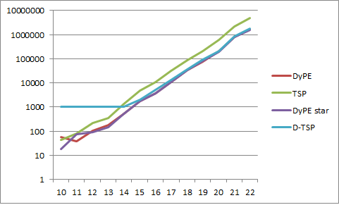
Figure 4 presents very preliminary simulation results.

References

- [1] Bistaffa, F., Farinelli, A., Cerquides, J., Rodríguez-Aguilar, J., and Ramchurn, S. D. 2014. Anytime coalition structure generation on synergy graphs. In Proceedings of the 13th International Conference on Autonomous Agents and Multi-agent Systems. AAMAS ’14. 13–20.
- [2] Michalak, T., Rahwan, T., Sroka, J., Dowell, A., Wooldridge, M., McBurney, P., and Jennings, N. R. 2009. On representing coalitional games with externalities. In ACM EC ’09: Tenth ACM Conference on Electronic Commerce. 11–20.
- [3] Myerson, R. 1977. Graphs and cooperation in games. Mathematics of Operations Research 2, 3, 225–229.
- [4] Rahwan, T. and Jennings, N. R. 2008. An improved dynamic programming algorithm for coalition structure generation. In AAMAS’08: Seventh International Conference on Autonomous Agents and Multi-Agent Systems. 1417–1420.
- [5] Rahwan, T., Michalak, T., Elkind, E., Wooldridge, M., and Jennings, N. R. 2014. An exact algorithm for coalition structure generation and complete set partitioning. http://www.cs.ox.ac.uk/publications/publication6962-abstract.html.
- [6] Rahwan, T., Michalak, T., and Jennings, N. R. 2012. A hybrid algorithm for coalition structure generation. In Proceedings of the 26th AAAI Conference on Artificial Intelligence (AAAI-2012).
- [7] Rahwan, T., Michalak, T., Wooldridge, M., and Jennings, N. R. 2012. Anytime coalition structure generation in multi-agent systems with positive or negative externalities. Artificial Intelligence 186, 0, 95 – 122.
- [8] Rahwan, T., Michalak, T., Wooldridge, M., and Jennings, N. R. 2015. Coalition structure generation: A survey. Artificial Intelligence 229, 0, 139 – 174.
- [9] Rahwan, T., Ramchurn, S. D., Giovannucci, A., and Jennings, N. R. 2009. An anytime algorithm for optimal coalition structure generation. Journal of Artificial Intelligence Research (JAIR) 34, 521–567.
- [10] Vinyals, M., Voice, T., Ramchurn, S., and Jennings, N. R. 2013. A hierarchical dynamic programming algorithm for optimal coalition structure generation. http://arxiv.org/abs/1310.6704.