Intervalley coupling by quantum dot confinement potentials in monolayer transition metal dichalcogenides
Abstract
Monolayer transition metal dichalcogenides (TMDs) offer new opportunities for realizing quantum dots (QDs) in the ultimate two-dimensional (2D) limit. Given the rich control possibilities of electron valley pseudospin discovered in the monolayers, this quantum degree of freedom can be a promising carrier of information for potential quantum spintronics exploiting single electrons in TMD QDs. An outstanding issue is to identify the degree of valley hybridization, due to the QD confinement, which may significantly change the valley physics in QDs from its form in the 2D bulk. Here we perform a systematic study of the intervalley coupling by QD confinement potentials on extended TMD monolayers. We find that the intervalley coupling in such geometry is generically weak due to the vanishing amplitude of the electron wavefunction at the QD boundary, and hence valley hybridization shall be well quenched by the much stronger spin-valley coupling in monolayer TMDs and the QDs can well inherit the valley physics of the 2D bulk. We also discover sensitive dependence of intervalley coupling strength on the central position and the lateral length scales of the confinement potentials, which may possibly allow tuning of intervalley coupling by external controls.
pacs
73.22.-f, 73.21.La, 73.61.LeI Introduction
Semiconductor quantum dots (QDs) have been widely explored in the past several decades for technological applications such as lasers and medical markers [Tartakovskii_Tartakovskii_2012____Quantum]. Spin and other quantum degrees of freedom of single electron or hole confined in QDs are also extensively researched as potential carriers of information for quantum computing and quantum spintronics [Hanson_Vandersypen_2007_79_1217__Spins, Liu_Sham_2010_59_703__Quantum, Loss_DiVincenzo_1998_57_120__Quantum, Reimann_Manninen_2002_74_1283__Electronic, Burkard_Loss_1999_59_2070__Coupled]. QDs in conventional semiconductors are realized either by forming nanocrystals or by lateral confinements in two-dimensional (2D) heterostructures. Such lateral confinements can be provided by the thickness variations of the heterostructures or patterned electrodes [Liu_Sham_2010_59_703__Quantum, Hanson_Vandersypen_2007_79_1217__Spins]. The emergence of graphene [CastroNeto_Geim_2009_81_109__electronic, Geim_Novoselov_2007_6_183__rise], the 2D crystal with single atom thickness, has offered a new system to host QDs. Because of the zero gap nature of graphene, QD confinement has to be facilitated by terminations of the monolayer, and the various geometries explored include the graphene nano-island connected to source and drain contacts via narrow graphene constrictions [Ponomarenko_Geim_2008_320_356__Chaotic, Guttinger_Ensslin_2009_103_46810__Electron, Wang_Chang_2011_99_112117__Gates], and graphene nanoribbon of armchair edges with patterned electrodes [Trauzettel_Burkard_2007_3_192__Spin]. The properties of these graphene QDs are affected significantly by the edges, and precise control on edge terminations are thus desired.
Monolayer group-VIB transition metal dichalcogenides (TMDs) are newly emerged members of the 2D crystal family [Wang_Strano_2012_7_699__Electronics]. These TMDs have the chemical composition of MX2 (M = Mo,W; X = S,Se), and the monolayer has a structure of X-M-X covalently bonded hexagonal quasi-2D network. The 2D bulk has a direct bandgap in the visible frequency range [splendiani_emerging_2010, mak_atomically_2010], ideal for optoelectronic applications. This bandgap also makes possible the realization of QDs without the assistance of termination edges [Kormanyos_Burkard_2014_4_11034__Spin]. QDs can be defined by lateral confinement potentials on an extended monolayer, e.g. by patterned electrodes, similar to the QDs in III-V heterostructures [Hanson_Vandersypen_2007_79_1217__Spins]. As the conduction and valence band edges are shifted in the same way by the electrodes, the QDs will have a unique type-II band alignment with its surroundings (cf. figure 1). Moreover, QD confinement potentials can also be realized by the lateral heterojunctions between different TMDs within a single uniform crystalline monolayer. Various band alignment can form between different TMDs with different bandgaps and workfunctions. Lateral heterostructures with MoSe2 islands surrounded by WSe2 on a crystalline monolayer has been realized very recently [Huang_Xu_2014____Lateral]. This can realize QD confinement, also with type-II band alignment, for electrons at the MoSe2 region. The band edge discontinuity at the heterojunction, with an order of magnitude of 0.2–0.4 eV [Rivera_Xu_2014___1403.4985_Observation, Lee_Kim_2014___1403.3062_Atomically, Furchi_Mueller_2014___1403.2652_Photovoltaic, Cheng_Duan_2014___1403.3447_Electroluminescence, Fang_Javey_2014___1403.3754_Strong], forms the potential well (with a vertical wall).
Besides the unique 2D geometries, monolayer TMD QDs are highly appealing because of the interesting properties of the 2D bulk. The conduction and valence band edges are both at the degenerate and valleys at the corners of the hexagonal Brillouin zone. Remarkably, the direct-gap optical transitions are associated with a valley dependent selection rule: left- (right-) handed circular polarized light excites interband transitions in the () valley only [Yao_Niu_2008_77_235406__Valley, Xiao_Yao_2012_108_196802__Coupled]. Based on this selection rule, optical pumping of valley polarization [zeng_valley_2012, mak_control_2012, cao_valley_selective_2012], and optical generation of valley coherence [Jones_Xu_2013_8_634__Optical], have been demonstrated. Another remarkable property of the 2D TMDs is the strong interplay between spin and the valley pseudospin [Gong_Yao_2013___1303.3932_Magnetoelectric, Jones_Xu_2014_10_130__Spin, Xu_Heinz_2014____]. These quantum degrees of freedom with versatile controllability well suggest that single electron in monolayer TMD QDs can be promising carrier of information for quantum spintronics, provided that the bulk properties of interest can be inherited by the QDs. Since these interesting bulk properties are associated with the valley pseudospin, a central problem is whether valley is still a good quantum number and whether the bulk valley physics is preserved in the QDs. A natural concern is that the lateral QD confinement may result in valley hybridization, like in silicon QDs [Saraiva_Koiller_2009_80_81305__Physical, Koiller_Das_2004_70_115207__Shallow, Goswami_Eriksson_2007_3_41__Controllable, Friesen_Coppersmith_2010_81_115324__Theory, Culcer_Das_2010_82_155312__Quantum, Friesen_Coppersmith_2007_75_115318__Valley, Nestoklon_Ivchenko_2006_73_235334__Spin, Boykin_Lee_2004_84_115__Valley], which may completely change the valley physics in QDs.
In this paper, we present a systematic study on the intervalley coupling strength by QD confinement potentials on extended TMD monolayer. The numerical calculations used two methods: (i) the envelope function method (EFM) [Kohn_canonical_transformation, Pantelides_Sah_1974_10_621__Theory, DiVincenzo_Mele_1984_29_1685__Self, Wang_Zunger_1999_59_15806__Linear], in conjunction with first-principles wavefunctions of the band-edge Bloch states of the 2D bulk; and (ii) the real-space tight-binding (RSTB) approach based on a three-band model for monolayer TMDs [Liu_Xiao_2013_88_85433__Three]. The EFM is limited to circular shaped QDs and is used primarily as a benchmark for the RSTB approach which can handle arbitrarily shaped QDs. The intervalley coupling is defined here as the off-diagonal matrix element, due to the QD potentials, between states with the same spin but opposite valley index. For circular QD potentials with various lateral size, potential depth and smoothness, the intervalley couplings from the two different approaches agree well, which justify both methods. We then use the RSTB method to address QD potentials of lower symmetry, including the triangular, hexagonal, and square shaped QDs, where the intervalley coupling strength is investigated as functions of lateral size, depth and smoothness of confinement potentials.
Our main findings are summarized below. For confinement potentials with the rotational symmetry (like that of the lattice), both the numerical results and the symmetry analysis show that the intervalley coupling strength depends sensitively on the central position of the potential: the coupling is maximized (zero) if the potential is centered at a M (X) site (cf. figure 1). The results stated below refer to the M-centered potentials. The intervalley coupling as a function of the lateral size of the QDs exhibits fast oscillations with an nearly exponentially decaying envelop. When the wall of the potential well changes from a vertical one to a sloping one, the intervalley coupling strength has a fast decrease by 2-3 orders of magnitude, and saturates when the length scale of the slope is beyond five lattice constants. For potentials with sloping walls, the intervalley coupling increases with increasing the potential depth. For potentials with vertical walls, the dependence on the potential depth is non-monotonic. Interestingly, when all parameters are comparable, the intervalley coupling can be smaller by several orders of magnitude in certain QD potentials. These include the circular shaped QDs, the triangular and hexagonal shaped QDs with all sides along the zigzag crystalline axes. The latter two types of confinement potentials can be relevant in QDs formed by lateral heterostructures of different TMDs [Huang_Xu_2014____Lateral]. In contrast to graphene QDs [Trauzettel_Burkard_2007_3_192__Spin] and silicon QDs [Saraiva_Koiller_2009_80_81305__Physical, Koiller_Das_2004_70_115207__Shallow, Goswami_Eriksson_2007_3_41__Controllable, Friesen_Coppersmith_2010_81_115324__Theory, Culcer_Das_2010_82_155312__Quantum, Friesen_Coppersmith_2007_75_115318__Valley, Nestoklon_Ivchenko_2006_73_235334__Spin, Boykin_Lee_2004_84_115__Valley], the intervalley coupling here is much smaller as the electron wavefunction vanishes at the boundary of QDs. For all QDs studied, the largest intervalley coupling is upper bounded by 0.1 meV, found for small QDs with diameters of 20 nm and with confinement potentials of vertical walls. Such intervalley coupling is much smaller compared to the diagonal energy difference between states with the same spin but opposite valley index, which arises from the spin-valley coupling and ranges from several to several tens meV in different monolayer TMDs [Liu_Xiao_2013_88_85433__Three]. Therefore, our results mean that valley hybridization is in general negligible, and valley pseudospin in monolayer TMD QDs is a good quantum degree of freedom as in the 2D bulk, with the optical addressability for quantum controls.
The rest of the paper is organized as follows. In section II, we formulate the EFM for the two-band model of the monolayer TMDs [Xiao_Yao_2012_108_196802__Coupled], which can be exactly solved for circular shaped QDs. We then present the numerical results for intervalley coupling, calculated in conjunction with the first-principles wavefunctions. In section III, we present the symmetry analysis on the M-centered and X-centered potentials with rotational symmetry. Section IV is on the RSTB approach. Numerical results by RSTB method for circular QDs are first compared with the EFM results, and then the RSTB results for various shaped QDs is presented. The results are qualitatively the same and quantitatively comparable for different MX2, and MoS2 is presented as the example throughout the paper.
II Circular QDs in envelope function method
II.1 The model and method

We consider first a QD defined by a circular shaped potential in a TMD monolayer. Such confinement potential can be characterized by three parameters: the lateral size, the depth, and the smoothness of the potential well. Without loss of generality, we assume the potential has the form
| (1) |
where and are respectively the lateral size and the depth of the potential well. characterizes the smoothness of the potential well boundary [see figure 1(c)]. Large corresponds to smooth potentials (e.g. in confinement generated by patterned electrodes), while corresponds to potential well with vertical wall (e.g. in lateral heterostructures of different TMDs). The parameter is used here.
For typical confinement with much larger than the lattice constants, the bound states in the QDs are formed predominantly from the band-edge Bloch states in the valleys of the 2D bulk. In the EFM, we start off with the two-band Hamiltonian derived for the band edges at the valleys of monolayer TMDs [Xiao_Yao_2012_108_196802__Coupled, Liu_Xiao_2013_88_85433__Three], where valley is a discrete index. Thus the EFM leads to confined wavefunctions formed with the and valley Bloch states respectively, denoted as where is the valley index denoting the valley, and or is the spin index. Taking these states as the basis, intervalley coupling here refers to the off-diagonal matrix elements between these states due to the confinement potential [Saraiva_Koiller_2009_80_81305__Physical].
As confinement potential is spin-independent, intervalley coupling vanishes between states with opposite spin index. For holes, the band edges of the 2D bulk are spin-valley locked because of the giant spin-orbit coupling [zhu_giant_2011, Xiao_Yao_2012_108_196802__Coupled], i.e. valley () has spin up (down) only. Thus, intervalley coupling is absent for holes. We concentrate on the intervalley coupling of confined electron states and in the two valleys with the same spin index, which is defined as
| (2) |
here is the off-diagonal matrix element, due to the QD potentials, between states with the same spin but opposite valley index. This quantity determines to what degree the two bulk valleys can hybridize in the QD confinement, by competing with the diagonal energy difference between and . If is much smaller than the diagonal energy difference, then the bulk valley index is still a good quantum number in QD. If the coupling is comparable or larger than the diagonal energy difference, then the QD eigenstates will be superpositions of the two bulk valleys. In the limit that is much larger than the diagonal energy difference, the QD eigenstates are the symmetric and antisymmetric superpositions of the two valleys, and their energy splitting is given by . Due to the time-reversal symmetry, . Hence we consider here only spin-up case and drop the spin index in superscripts for brevity.
To obtain in EFM, we substitute for in the Hamiltonian of the 2D bulk[Xiao_Yao_2012_108_196802__Coupled, Liu_Xiao_2013_88_85433__Three], and the confinement potential is added as an onsite energy term. The QD Hamiltonian in each valley is then [Hewageegana_Apalkov_2008_77_245426__Electron, Pereira_Peeters_2007_7_946__Tunable, Chen_Chakraborty_2007_98_186803__Fock, Matulis_Peeters_2008_77_115423__Quasibound, Recher_Trauzettel_2009_79_85407__Bound, Pereira_Farias_2009_79_195403__Landau, Hewageegana_Apalkov_2009_79_115418__Trapping]
| (3) |
where eV is the bulk bandgap of TMD monolayer, is the lattice constant, and is the effective hopping. The bases of the Hamiltonian (3) are the conduction and valence Bloch states at point, (c, v and is the cell periodic part), and the eigenfunction of (3) is a spinor of envelope function
| (4) |
which satisfy the Schrodinger equation . The overall wavefunctions of the QD states are then
| (5) |
Since has the rotational symmetry, it is easy to verify that the eigen spinor is of the form
| (6) |
where is integer, and are the polar coordinates of . and are real radial functions that satisfy
| (7) |
and are Bessel functions in the region where is a constant ( or ), and need to be solved numerically in the region . Boundary conditions are then matched at and to determine the solutions and eigenvalues. Bound states are found to exist in the energy range , as expected. Here is used as the unit of energy and as the unit of length.
| (9) |
| (10) |
and
| (11) |
In the above equations, {c, v}, and are the Fourier coefficients of the periodic part of the Bloch function . is a reciprocal lattice vector (RLV), and is also a RLV. Here we are interested in the QD ground states only, which correspond to the case in equation (10) [see figure 2(a)]. The coefficients are obtained here from the first-principles all-electron wavefunctions calculated by the ABINIT package [abinit1, note2].
We note that the Hamiltonian in equation (3) does not contain the conduction band spin-valley interaction [Liu_Xiao_2013_88_85433__Three, Kormanyos_Falko_2013_88_45416__Monolayer], which is of the Ising form that changes only the diagonal energies but not the wavefunctions of the states and . Thus, this spin-valley interaction does not affect the intervalley coupling strength defined here, but it leads to an energy difference between states and that ranges from several to several tens meV [Liu_Xiao_2013_88_85433__Three, Kormanyos_Falko_2013_88_45416__Monolayer]. Valley hybridization in the QDs is determined by the competition between and this diagonal energy difference.
II.2 Numerical results
In this subsection we present the numerical calculation results. The parameters from [Xiao_Yao_2012_108_196802__Coupled] are used: eV, Å, eV, and eV. We consider potentials centered at a Mo site, as shown in figure 1(a). As we will prove in Section III, the intervalley coupling is strongest for such Mo-centered confinement potential, and will vanish if the circular confinement potential is centered at a S site.
II.2.1 Energy levels and bound states
We first look at the energy eigenvalues and eigenstates of equation (3), which give the energy spectrum in the circular QD confinement, and the radial envelope functions to calculate the intervalley coupling [cf. equation (2)]. The energy spectra are shown in figure 2(a) for , and three well depths0.2, 0.05, and 0.005. For and 0.05, only the low-energy parts of the spectra are shown. is the azimuthal quantum number of the envelope function defined in equation (6). Obviously, the ground state has . The spectra shown are for the valley () and it is obvious from equation (7) that states of , , are degenerate with states of , . For the ground states, the radial envelope functions and are shown in figure 2(b), from which we can see that they are smooth and localized within the well and the components are orders of magnitude smaller compared to . This means that for electron confined in the quantum dot, the wavefunction is predominantly contributed by the conduction band edge Bloch functions, and the contribution from the valence band edge is negligible. In general, the Hamiltonian (3) shall be solved for addressing confinement of Dirac fermions, as we did here. Nevertheless, as shown here, the much simplified approach of effective mass approximation can be well justified for monolayer TMDs with the large bandgap. Importantly, the wavefunction has vanishing amplitude at the QD boundary [green shaded region in figure 2(b)]. This is in contrast to the wavefunctions in graphene QDs [Trauzettel_Burkard_2007_3_192__Spin] and silicon QDs [Saraiva_Koiller_2009_80_81305__Physical, Koiller_Das_2004_70_115207__Shallow, Goswami_Eriksson_2007_3_41__Controllable, Friesen_Coppersmith_2010_81_115324__Theory, Culcer_Das_2010_82_155312__Quantum, Friesen_Coppersmith_2007_75_115318__Valley, Nestoklon_Ivchenko_2006_73_235334__Spin, Boykin_Lee_2004_84_115__Valley] where significant valley hybridization is found.
II.2.2 The intervalley coupling
With the envelope functions given above, and the band-edge Bloch functions from the ABINIT package [abinit1, note2], we can calculate the numerical values for the intervalley coupling [cf. equation (8)],
Figure 3 shows the intervalley coupling strength versus the radius of the potential for circular QDs with fixed smoothness ( and 10) and depth () of potential [cf. equation (1)]. The curve with is more than two orders of magnitude smaller than the one with , which can also be seen in figure 4 and discussed in detail later. From figure 3(b) and (c), we can see that the dominant contribution to the intervalley coupling is from , which is orders of magnitude larger than , , [cf. equation (9)], consistent with the fact that the wavefunction of confined electron is predominantly from the conduction band edge Bloch functions. Figures 3(b) and (c) also clearly show that oscillates vs in the scale of the lattice constant . The oscillation with the size of QD is a generic feature of intervalley coupling, due to the large momentum space separation of the two valleys, which have been noted in previous works [Boykin_Lee_2004_84_115__Valley, Nestoklon_Ivchenko_2006_73_235334__Spin, Friesen_Coppersmith_2007_75_115318__Valley]. Apart from these fast oscillations, the intervalley coupling strength decreases with the increase of in a nearly exponential way.
Figure 4 shows the as a function of , the smoothness of the potential, for circular QDs with and . Largest intervalley coupling is found at that corresponds to a circular square well, where the potential has a sudden jump at the QD boundary. It can be seen that decreases monotonically as increases up to a value of 5, and then it starts to oscillate rapidly around a constant value. The inset is the zoom in for , which shows that the oscillation is also in the length scale of lattice constant, similar to the vs. relation.
Figure 5 shows the dependence of on the potential depth , when and and 10. We can see that increases with increasing when , and it first increases and then decreases with increasing when . In this figure, we also compare the intervalley couplings calculated with and without spin-orbit coupling (SOC). For the calculation without SOC, we set in equation (3), and the plane-wave coefficients in equation (11) are also calculated without including the SOC in the ABINIT package. In figure 5, it is clear that intervalley couplings with and without SOC coincide when , and have small difference when . We also compared the vs. curve (fixing , ) and vs. curve (fixing , ), for the calculations with and without SOC, and the differences are also negligible. This means that SOC has negligible effects on . This is well expected as here is just the off-diagonal matrix element of the confinement potential, between the QD wavefunctions in the and valleys. The SOC in the valleys is of the longitudinal form [Xiao_Yao_2012_108_196802__Coupled], which does not affect the wavefunction. The SOC, however, will cause spin splittings and hence affect the spectral of quantum dot states in the and valleys [cf. figure 2(a)]. When we consider the effect of intervalley coupling on the quantum dot states, the off-diagonal matrix element will then compete with the differences in these diagonal energies, and the SOC induced spin splitting will play an important role.
From the dependence of on , , and discussed above, we find that the intervalley coupling strength in a circular confinement potential varies over several orders of magnitude, depending on the length scale, smoothness, and depth of the confinement. The magnitude of the intervalley coupling is small on the whole, in the order of eV or below. This is much smaller compared to intervalley coupling in QDs formed in silicon inversion layers [Saraiva_Koiller_2009_80_81305__Physical, Nestoklon_Ivchenko_2006_73_235334__Spin, Koiller_Das_2004_70_115207__Shallow, Goswami_Eriksson_2007_3_41__Controllable, Friesen_Coppersmith_2007_75_115318__Valley, Friesen_Coppersmith_2010_81_115324__Theory, Culcer_Das_2010_82_155312__Quantum, Boykin_Lee_2004_84_115__Valley].
III Symmetry analysis for QDs with rotational symmetry
In the above section, we have seen that the intervalley coupling is very sensitive to the geometry of the confinement potential, as evident from the fast oscillations of versus or . Here, based on symmetry analysis, we will show that the intervalley coupling strength also depends on the position of the potential center, in a way that is largest when the potential is centered at Mo atom [figure 1(a)] but vanishes if centered at S atom [figure 1(b)]. To explain this, we analyze [see equation (9)] by examining the behavior of and under the rotation.
Using the Fourier relation in which is the area of the 2D cell, can be rewritten as
| (12) | |||||
| (13) |
where . Equation (12) shows that its integrand is a cell periodic function. This periodicity leads to the invariance of under the rotation of its integrand. For convenience, we rewrite . Using the form of integrand in equation (13), we get
| (14) | |||||
where is the eigenvalue of operation corresponding to the Bloch function .
For the integral , we also rewrite it as . Using the integral form of the Bessel function of order (integer) , we can simplify to single integrals as
| (15) |
| (16) |
| (17) |
| (18) |
where is the polar angle of the 2D vector . It is obvious that under , the integral parts of equations (15)–(18) do not change, and hence the ratio is determined only by the prefactor in front of the integrals:
| (19) |
Because the set of ’s, , also has the symmetry, we can choose one third elements of , denoted as , such that . Using equations (14) and (19), we have
| (20) | |||||
where
| (21) |
is already given in equation (19) and the rest is to determine .
For MoS2 monolayer, the conduction and valence band edge Bloch functions at points are formed predominantly by the (i.e. ) and [i.e. ] orbitals of Mo atoms respectively [Xiao_Yao_2012_108_196802__Coupled, Liu_Xiao_2013_88_85433__Three, note2]. There are two contributions to the eigenvalue of the rotation on the Bloch function (details in Appendix A): (i) the rotation of atomic orbital around its own center, i.e. and ; (ii) the change of lattice phase, defined as the value of the planewave phase factor at each lattice site (cf. figure 1 for the case of ). The change of the lattice phase factor under rotation depends on the rotation center. If the rotation center is at Mo atom as shown in figure 1(a), the rotation does not change the lattice phase factors leaving only contribution (i) taking effect, and we obtain
| (22) |
However, if the rotation center is at S atom, as shown in figure 1(b), both contributions (i) and (ii) take effect and we have
| (23) |
Putting equations (19) and (22) [or (23)] into equation (21), we obtain that for Mo centered potential and for S centered potential, and the final intervalley coupling is
| (24) |
From the above symmetry analysis, we conclude that the intervalley coupling induced by a circular confinement potential is sensitive to the center of the potential. The intervalley coupling is enhanced when the potential is centered at Mo atom, while it vanishes if the potential is centered at S atom. This is due to the dependence of , the eigenvalue of the Bloch function under the rotation, on the location of rotation center. Below, we show that the same conclusions can be drawn as long as the confinement potential has the symmetry, i.e. intervalley coupling is strongest (zero) if the center of the potential is at Mo (S) site.
III.1 Noncircular QD with symmetry
Consider a noncircular QD confinement potential with symmetry only, . In such potential that lacks the circular symmetry, we do not have exact solution in general for the massive Dirac Fermion Hamiltonian in equation (3). Nevertheless, the numerical results presented in section II.2 have well justified the effective mass approximation, where we can construct the QD electron wavefunction based on the conduction band edge Bloch function only. The ground-state envelope function can be obtained by solving the following effective-mass Hamiltonian
| (25) |
where is the effective mass of conduction band at . With the same at , the envelope functions in the two valleys are the same: . To analyze the symmetry, we need to know and [see equations (20) and (21)]. is independent of the shape of the QD, and equations (22) and (23) are still valid here. is determined by the symmetry of the envelope function . Since is symmetric under rotation, the non-degenerate ground-state envelope function in each valley has to be an eigenstate of , i.e. where . Using equation (10) and , we have
| (26) | |||||
Thus , consistent with equation (19). The conclusion of equation (24) is therefore valid for QD confinement potential with symmetry.
In summary, the band edge Bloch functions at and have the rotational symmetry of the lattice. However, they transform differently when the rotation center is Mo site or S site, as shown in Figure 1a and 1b respectively. When the QD confinement potential also has the rotational symmetry about a S site, the rotational symmetry of the band edge Bloch functions about the S site leads to destructive interference and hence vanishing intervalley coupling. This is the physical origin of the dependence of intervalley coupling on the central position of QD potential.
IV Real-space tight-binding method
In the EFM, except for the circular shaped confinement potential, it is difficult to find the exact wavefunction of the bound states in the QD. To investigate the intervalley coupling in the more general case of the QDs with noncircular shape, we consider here the alternative approach of real-space tight-bind (RSTB) method. Using RSTB, we first calculate intervalley couplings of circular shaped QDs and compare with the results from EFM. The agreement between the two methods well justifies the validity of the RSTB method. Then we calculate intervalley couplings of noncircular shaped QDs and analyze the results. Since SOC has negligible effects on intervalley coupling, we did not take into account SOC in the RSTB calculation.
IV.1 The RSTB model
We use supercell and periodic boundary condition to model a QD. The supercell is a square with side length (cf. figure 9). Each supercell has lattice points for primitive cells. All lengths are in unit of lattice constant . We adopt the three-band tight-binding model developed in [Liu_Xiao_2013_88_85433__Three], considering hoppings between nearest-neighbour Mo-, , and orbitals. The coordinates of the lattice sites of Mo atoms are denoted as . The tight-binding Hamiltonian of the QD is
| (27) |
where is the QD confinement potential at , are orbital indices, is the creation operator for electron on site with orbital . is the hopping between orbital at position and orbital at position , and denotes summation over nearest-neighbor pairs only. In practice, we write the Hamiltonian in form of a matrix. The part of involving hoppings between site and can be written as a block , where is either or the six nearest-neighbour vectors to defined in [Liu_Xiao_2013_88_85433__Three]. Using the real hopping parameters defined in [Liu_Xiao_2013_88_85433__Three] (the GGA-version parameters therein), we have,
| (28) |
| (29) |
| (30) |
| (31) |
The RSTB Hamiltonian matrix for a QD is then diagonalized to find the eigenstates and eigenenergies.
Unlike the EFM approach where the bound state wavefunctions are first given in each valley, and the intervalley coupling then calculated as the off-diagonal matrix element between them [cf. equation (2)], the eigenstates and eigenenergies of the RSTB Hamiltonian already include the effects of intervalley coupling. The intervalley coupling causes a fine splitting of the energy levels, which otherwise have the two-fold valley degeneracy in the absence of SOC. This energy splitting is just . Thus, the magnitude of the intervalley coupling is read out from the difference between the lowest two conduction-band energy eigenvalues of in the RSTB solution [note1].
IV.2 Circular shaped QDs
We study here circular shaped QDs using RSTB and compare with the results in EFM. First, we check the impact of supercell size on the intervalley coupling. Figure 6 shows the vs. relation for different circular QDs. We can see that converges fast with increasing , which means that the finite-size effects introduced by the method can be well eliminated by having large enough supercell. Figure 6 also shows that converges faster with increasing for larger potential depth , just as expected.
calculated using RSTB method with a large supercell () is compared with the results from EFM in figure 7. For the vs. dependence [figure 7(a)], the vs. dependence [figure 7(b)], and the vs. dependence [figure 7(c)], the RSTB data, including the rapid local oscillations, agree quantitatively well with the EFM ones. The EFM results rely on the details of the first-principles wavefunctions of Bloch states from the ABINIT package, while the RSTB calculations are based on a few hopping matrix elements only. This agreement between the two entirely different approaches well justify both the RSTB method and EFM.
In figure 8, we analyze the dependence of the intervalley coupling strength on the central position of the confinement potential. Figure 8(a) shows vs. curves of the same circular shaped potential centered at a Mo or S site. Consistent with the symmetry analysis in Section III, is three orders of magnitude larger for the Mo-centered case compared to the S-centered ate, the latter can be regarded as the numerical errors from zero. Figure 8(b) plots as a function of the central position of the confinement potential. Clearly, decreases when the potential center moves away from the Mo site and eventually vanishes when the potential center is at the S site.
IV.3 Intervalley coupling in noncircular QD potentials with vertical wall ()
QDs can be formed by the lateral heterostructures between different monolayer TMDs. Currently such heterostructures are grown by chemical vapor deposition (CVD), where the shape of confinement is triangular [Huang_Xu_2014____Lateral]. The lateral size of the confinement in available heterostructures is several m, still too large for QDs. Nevertheless, growth of monolayer TMDs flakes with sizes ranging from tens of nm to tens of m and with both triangular and hexagonal shapes have been reported by various groups [Helveg_Besenbacher_2000_84_951__Atomic, bollinger_one_dimensional_2001, Zande_Hone_2013_12_554__Grains, Peimyoo_Yu_2013_7_10985__Nonblinking, Najmaei_Lou_2013_12_754__Vapour, Cong_Yu_2014_2_131__Synthesis, Wu_Xu_2013_7_2768__Vapor, Gutierrez_Terrones_2013_13_3447__Extraordinary]. Smaller QDs formed by the lateral heterostructures can be well expected. In such heterostructures, the confinement potential is due to the band edge difference between the TMDs. Thus the potential well has a vertical wall at the QD boundary, corresponding to the limit discussed above. Here we use RSTB method to investigate intervalley coupling of these noncircular QDs. We studied QDs with triangular, hexagonal as well as the square shapes for comparison.
As shown in figure 9, the triangular, hexagonal, and square QDs are defined by the confinement potentials , , and respectively, where equals to 0 within the QDs (yellow regions), and equals to the constant outside (white regions). The ’radius’ of the QDs is denoted as (see figure 9). For the triangular and hexagonal QDs, we have chosen the orientation of the confinement potential such that the sides are all along the zigzag crystalline axes, corresponding to those realizable by the lateral heterostructures of different dichalcogenides. For the square QDs, two sides are along the zigzag and the others are along the armchair crystalline axes.
Figure 10 plots the intervalley coupling as function of the QDs size, for three different potential depthseV, eV and eV. With increasing , the intervalley coupling strength has an overall trend to decrease, but with rapid local oscillations. These features are similar to the circular QDs (cf. figure 3). Interestingly, for the triangular and hexagonal QDs, intervalley coupling is found to be much smaller with the larger potential jump at the QD boundary. In figure 11, the dependence of the intervalley coupling on is investigated, in which all curves are non-monotonic. The non-monotonic dependence of intervalley coupling strength is also found for the circular QDs when (cf. figure 5). We note that in heterostructures formed between different monolayer dichalcogenides (e.g. MoSe2 and WSe2), the conduction and valence band edge discontinuities are discovered to be in the range of 0.2–0.4 eV [Rivera_Xu_2014___1403.4985_Observation]. For this range of values for , the intervalley coupling is well negligible for the triangular and hexagonal QDs.
Comparing QDs of different shapes, the intervalley coupling in square QDs is orders of magnitude larger than that in the triangular and hexagonal QDs. Such a sharp difference is due to the relative orientation of the sides of the confinement potential to the crystalline axes. Inhomogeneous junctions along the zigzag (armchair) crystalline axes preserves the momentum along (perpendicular to) the lines connecting the two valleys in the momentum space. Thus, the zigzag junctions introduce the minimum intervalley coupling, while the armchair junctions cause maximum intervalley coupling. For the triangular and hexagonal QDs, all sides are along the zigzag crystalline axes, while for square QDs two sides are along the armchair directions and thus intervalley coupling is much larger. This is further verified by examine the change of the intervalley coupling when we rotate the QD confinement potential by an angle relative to the orientation defined in figure 9, as shown in figure 12. For triangular and hexagonal QDs, we find the intervalley coupling increases with significantly, and reaches a maximum at where the intervalley coupling becomes comparable with the square QDs. Note that at , the sides of the confinement potential of the triangular and hexagonal QDs are along the armchair crystalline axes [cf. figure 12(a) and (b)].
Figure 13 shows the dependence of on the central position of the confinement potential in a unit cell for the three kinds of noncircular QDs. It is clear that strongly depends on the potential center. For triangular and hexagonal QDs with the rotational symmetry, the dependence is similar to the circular QDs [cf. figure 8(b)], i.e. intervalley coupling is strongest if the potential is centered at a Mo site, but vanishes if the potential is centered at a S site. Such behavior is absent for the square QDs that lacks the rotational symmetry.
IV.4 Intervalley coupling in smooth noncircular QD potential
Finally, we examine square shaped QDs but with a smooth slope for the potential change on the boundary (i.e. finite ), which represents a general situation for QDs defined by patterned electrodes. The calculated intervalley coupling strength as a function of QD size is shown in figure 14. The peak value of intervalley coupling decreases nearly exponentially with the QD size. The dependence on the smoothness is similar to the circular shaped QDs (cf. figure 4), i.e. drops fast by several orders of magnitude when increases from 0 to 5, and becomes largely independent of for . From figure 14, we can see that the curves as functions of for , , and are basically the same, except for the location of some fine dips.
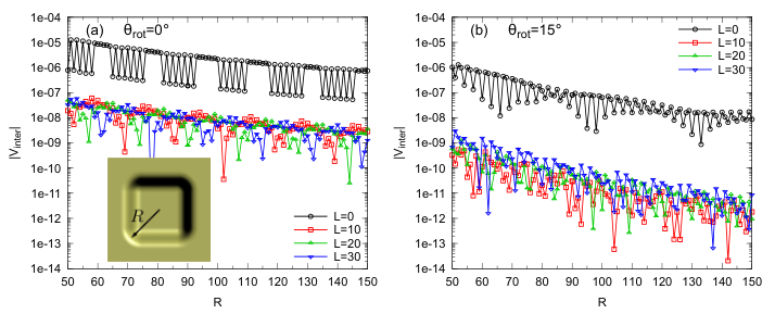
V conclusions and discussions
To conclude, we have investigated intervalley coupling in QDs defined by confinement potentials of various shapes on extended TMD monolayer. The numerical results obtained using two completely different approaches agree well with each other. For confinement potentials with the rotational symmetry, the intervalley coupling is maximized (zero) if the potential is centered at a M (X) site. Comparing smooth confinement potentials with slopping walls and sharp confinement potentials with vertical walls, the intervalley coupling in the latter is much stronger. When the length scales of the QDs vary, the intervalley coupling exhibits fast oscillations where the maxima can be two orders of magnitude larger than the neighboring minima, and the envelop of the maxima has an overall nearly exponential decay with the increase of the QDs size. When all parameters are comparable, the intervalley coupling can be smaller by several orders of magnitude in circular shaped QDs, and in triangular and hexagonal shaped QDs with all sides along the zigzag crystalline axes. For all QDs studied, the largest intervalley coupling is upper bounded by 0.1 meV, found for small QDs with diameters of 20 nm and with sharp confinement potentials (i.e. vertical walls).
The intervalley coupling in these monolayer TMD QDs is much smaller compared to that in graphene nanoribbon QDs [Trauzettel_Burkard_2007_3_192__Spin] and in silicon QDs [Saraiva_Koiller_2009_80_81305__Physical, Koiller_Das_2004_70_115207__Shallow, Goswami_Eriksson_2007_3_41__Controllable, Friesen_Coppersmith_2010_81_115324__Theory, Culcer_Das_2010_82_155312__Quantum, Friesen_Coppersmith_2007_75_115318__Valley, Nestoklon_Ivchenko_2006_73_235334__Spin, Boykin_Lee_2004_84_115__Valley]. In QDs formed in 2D crystals, intervalley coupling mainly occurs at the boundary where the translational invariance is lost, thus the coupling strength is proportional to the probability distribution of the electron at the QD boundary. In the TMD QDs studied here, the electron wavefunction has vanishing amplitude at the QD boundary [cf. green shaded region in figure 2(b)]. This is a characteristic of the QDs defined by confinement potentials on an otherwise extended crystalline monolayer, as opposed to the nanoribbon QDs [Trauzettel_Burkard_2007_3_192__Spin]. The geometry here is also qualitatively different from the QDs formed in silicon inversion layers. In those silicon QDs, the two valleys are separated by a wavevector along -direction (perpendicular to the inversion layer), and their coupling is caused by the sharp confinement with a length scale of nm in the -direction [Saraiva_Koiller_2009_80_81305__Physical, Koiller_Das_2004_70_115207__Shallow, Goswami_Eriksson_2007_3_41__Controllable, Friesen_Coppersmith_2010_81_115324__Theory, Culcer_Das_2010_82_155312__Quantum, Friesen_Coppersmith_2007_75_115318__Valley, Nestoklon_Ivchenko_2006_73_235334__Spin, Boykin_Lee_2004_84_115__Valley]. Such confinement strongly squeezes the wavefunction, giving rise to its large amplitude at the interface where valley hybridization occurs, and hence there is a stronger intervalley coupling in the order of meV. In contrast, here it is the much larger lateral size of the QDs that determines the wavefunction amplitude at the QD boundary. We can expect that intervalley coupling is generically small in QDs defined by confinement potentials on otherwise extended monolayer.
Because of the very small intervalley coupling in the monolayer TMD QDs, valley hybridization is then well quenched by the much stronger spin-valley coupling of the electron in monolayer TMDs. As a result, the QDs can well inherit the valley physics of the 2D bulk such as the valley optical selection rules, making the valley pseudospin of single confined electron a perfect candidate of quantum bit. The sensitive dependence of intervalley coupling strength on the central position and the lateral length scales of the confinement potentials further makes possible the tuning of the intervalley coupling by external controls. The qualitative conclusions here are also applicable to QDs formed by confinement potentials on other 2D materials with finite gap.
Acknowledgements.
The work was supported by the Croucher Foundation under the Croucher Innovation Award, the Research Grant Council of HKSAR under Grant No. HKU705513P and HKU9/CRF/13G (G.B.L., H.P., and W.Y.); the NSFC with Grant No. 11304014, the National Basic Research Program of China 973 Program with Grant No. 2013CB934500 and the Basic Research Funds of Beijing Institute of Technology with Grant No. 20131842001 and 20121842003 (G.B.L.); the MOST Project of China with Grants Nos. 2014CB920903 and 2011CBA00100, the NSFC with Grant Nos. 11174337 and 11225418, the Specialized Research Fund for the Doctoral Program of Higher Education of China with Grants No. 20121101110046 (Y.Y.).Appendix A The eigenvalue of Bloch function under rotation
Here we give a derivation of , the eigenvalue of the Bloch function under the rotation. We first express in terms of linear combination of atomic orbitals (c, v),
| (32) |
in which is lattice vector, is the position of Mo atom in the unit cell, , and . According the definition of and using the orthogonality of (), we have
| (33) |
Summing over all Mo positions is equivalent to summing over all positions when the rotation center locates at either Mo or S site (see figure 1). Accordingly, with the substitution , the above equation becomes
| (34) |
Because is an element of the wave-vector group of , we have and consequently
| (35) |
Define , we have
| (36) |
Plugging equations (35) and (36) into (34), we obtain
| (37) |
and therefore
| (38) |
in which the factor comes from the rotation of atomic orbital around its own center and the factor comes from the change of the lattice phase of Mo atom after rotation. According to equation (38), when the rotation center locates at Mo [figure 1(a)], we have and hence [equation (22)]; when the rotation center locates at S [figure 1(b)], we have and hence [equation (23)].