Recombining binomial tree for constant elasticity of variance process
Hi Jun Choe, Jeong Ho Chu and So Jeong Shin
Department of Mathematics, Yonsei University, Seoul, Republic of Korea
ABSTRACT.
The theme in this paper is the recombining binomial tree to price
American put option when the underlying stock follows constant
elasticity of variance(CEV) process. Recombining nodes of binomial
tree are decided from finite difference scheme to emulate CEV
process and the tree has a linear complexity. Also it is derived
from the differential equation the asymptotic envelope of the
boundary of tree. Conducting numerical experiments, we confirm the
convergence and accuracy of the pricing by our recombining binomial
tree method.
As a result, we can compute the price of American put option under CEV model, effectively.
Keywords. Recombination, Binomial tree, Envelope, CEV model, American put option
1. INTRODUCTION
Black and Scholes[2] derived the celebrated option pricing formula under the assumption that underlying stock price follows Geometric Brownian Motion(GBM). Under this assumption the distribution of prices is lognormal and the volatility is constant. However, the empirical evidence does not support the assumptions in the lognormal distribution and the constant volatility. In other words, unlike the basic assumption of GBM, we observe that the implied volatility embedded in the market price of option changes according to the exercise price and expiration. This phenomenon is called ‘volatility smile’. CEV model can explain the ‘volatility smile’ phenomenon and can more closely approximate the real world than GBM. So CEV model has been a popular alternative stock process model and there have been many attempts for financial applications. The option pricing formula when the underlying stock process follows CEV model was derived by Cox and Ross[4]. The financial implications of the CEV model are studied by Beckers[1]. It was noted that CEV model can fit the volatility skew of stock options. Indeed, Cox and Ross[4] and Emanuel and MacBeth[7] derived a closed-form solution for European option when a positive elasticity is assumed. Schroder[10] simplified the formula. However computations involving the non-central chi-square distribution function are complicated, and as an attempt Schroder introduced an analytic approximation of option pricing for CEV model. The explicit formula is only useful for European vanilla options, not for American options and other exotic options. Therefore it is common practice that American option is computed by binomial tree method. Nelson and Ramaswamy[6] suggested a simple binomial process approximation to describe CEV process. But, as noted by Nelson and Ramaswamy ([6], p.418), their simple binomial process approximation proposed deteriorates as maturity is lengthened. To overcome such a computational burden, we propose a real simple and accurate binomial tree to estimate the value of American put options and so on. The novelty of our binomial tree is exact recombination for CEV model. From finite difference scheme for partial differential equation a recombining tree is made for CEV model.
Moreover it is well known that the early exercise valuation problem can be solved by the binomial tree method. The binomial tree is an efficient and powerful method for pricing American options in contrast to the partial differential equation method and other numerical methods such as Monte-Carlo simulation. Tomer Neu-Ner[11] discussed alternative methods of pricing and compared them with the binomial method. He claimed that the binomial tree method is an extremely valuable tool for option pricing under CEV model. The remainder of this paper is organized as follows. In section 2, we review briefly CEV model. Section 3 is the main part in this paper. First, we derive a partial differential equation which holds for any type of option. Second, we build a binomial tree to approximate the CEV process and to evaluate the American put option valuation. In other words, we introduce the structure of binomial tree which can exactly recombine. In section 4, we present numerical results and discuss about the convergence of binomial process built in chapter 3. In section 5, we compute American put option value under the CEV model by the recombining binomial tree. In the final section, we present the conclusion of this paper.
2. CONSTANT ELASTICITY OF VARIANCE MODEL
CEV model was proposed by Cox and Ross[4] as an alternative to the Black and Scholes[2] model(GBM). This model proposes the following relationship between stock price and volatility
It means that the elasticity of return variance with respect to stock price equals .
In CEV model, the stock price is assumed to be governed by the diffusion process:
Here, we denote the stock price at an instant of time as , the change in the stock price over the increment as . , and are positive constants. is Wiener process. We assume the stock pays no dividends.
If , then the volatility is . So in this case, CEV model is just GBM model. Otherwise, observe that volatility varies with moves in the stock price level and time. If , the volatility and stock price move in the same direction. If , the volatility increases as the stock price decreases. In this case, the probability distribution is similar to that observed for stock option with a heavy left tail. It is known, based on empirical data, that stock prices and volatility have an inversely relationship. So we only consider the situation when .
3. BINOMIAL TREE FOR CEV DIFFUSION
3.1. FINITE DIFFERENCE METHOD FOR BLACK-SCHOLES EQUATION
We consider the general stock process.
First, define a function that gives the option value for an asset price at any time with . The key idea is hedging to eliminate risk. We can obtain the following equation by doing similar arguments to obtain a Black-Scholes equation:
| (1) |
where is the risk free rate and it is constant and positive. We are to recognize that time goes backward in (1).
Second, we apply FDM to the above equation. FDM is a straightforward method for solving Partial Differential Equations(PDE). FDM requires the domain to be replaced by a grid. The key step in deriving FDM is to replace differential operators with finite difference operators. By plugging the difference formula into the PDE (1), a difference equation (2) is obtained:
| (2) |
Here, denotes the value of the option corresponding to asset price at node. The superscript indicates the time level.
By simplifying we obtain
So, we have the explicit form of as following
| (3) |
where
If the finite difference scheme corresponds to the binomial tree, we have to make , that is,
| (4) |
We observe that, if then .
3.2. STRUCTURE OF THE BINOMIAL TREE
In CEV model and by simplifying the equation (4), we obtain the essential recombination equation
| (5) |
Now, we build a recombining binomial tree of stock prices. The basic idea of binomial tree construction is as follows. Here, we let (=) denote the price of stock at i-time level (). Put , , . And and are determined from the equation (5).
Note that is underlying stock price at -th time step. We explain the procedure in detail. First, is the current stock price. Put . If is given, then two known values and , and one unknown value should satisfy the recombination equation (5) because the stock price follows CEV model. That is, the value is determined by the two known values , and the equation (5).
Now, put and . Again, the value is determined by the two known values , and the equation (5). Similarly we obtain as determined by , and the equation (5).
We describe one more step. Put , . We obtain as determined by the equation (5) with the two known values and plugged in. Similarly, putting and , we obtain by plugging the two known values and into the equation (5). Observe that , , satisfy the equation (5). Continuing in the same manner, we can build a binomial tree of stock price of CEV model. Observe that, once has been determined, the binomial tree is uniquely determined.
The largest benefit of the binomial tree constructed in this manner is as follows. This is a most natural and simplest binomial tree that allows exact recombining under CEV model. Cox & Rubinstein([5], p362) have constructed a binomial approximation for the CEV diffusion. However, it turns out that computation is not appropriate in their case because tree does not recombine and thus the number of nodes doubles at each time step. When the binomial tree does not recombine at each node, the computation is not efficient. On the other hand, the binomial tree in which recombining occurs at each level is efficient and speedy to compute because the number of nodes grows at most linearly with the number of time intervals. That is, in a recombining binomial process, the stock price can take possible values after periods, for .
3.3. FINDING THE FIRST VALUE OF TREE(Determine the increasing rate of the stock price )
Now we have a problem. How can we set the value of ? In other words, we have to tune the parameter(: move up factor) and explain why.
By using the Euler’s discretization
Take so that
Since is far larger than for a small , we can ignore the term to get
Note that if ,
So we set the value of .
3.4. PROBABILITY OF UPWARD MOVE AT EACH NODE
In the CEV model, the volatility is not constant but varies with the value of the underlying price. When the volatility varies with the value of the price, the probability of an upward move has to be recomputed at each node. Now, we compute the probability of an upward move at each node. For notational simplicity, let . Then the equation (4) becomes
On the other hand, in the process of binomial tree, we have
Here, is the increasing probability of the stock price at node. So, we obtain the following equation by comparing with (3)
Since , we also have
Let
then with very small error, we can write
Then the above equation becomes
Therefore, in CEV model, we have
| (6) |
4. NUMERICAL TEST
In section 3, we built a binomial tree to emulate CEV diffusion. It provides an efficiency tool to price options because it recombines exactly. At this point, we present the convergence of pricing by binomial tree by numerical experiments.
4.1. EUROPEAN PUT OPTION
We have stochastic differential equation representing CEV process as follows:
where , , and are parameters of risk free rate, dividend yield and elasticity, respectively. Under CEV model, the closed-form formulas for pricing of European call and put options are available. Cox[3] obtained that
when (or ), and Emanuel and MacBeth[7] derived that
when (or ) with
, , where and
is the cumulative distribution function of a noncentral chi-square
random variable with noncentrality parameter and
degrees of freedom.
Now we compare European put option value between analytic solution and binomial tree solution to check the convergence of the binomial tree solution.
| Analytic solution | Tree-time step=365 | Tree-time stpe 365*2 | |||||||||
|---|---|---|---|---|---|---|---|---|---|---|---|
| =1/4 | =1/2 | =1 | =1/4 | =1/2 | =1 | =1/4 | =1/2 | =1 | |||
| =0.5 | 0.5 | 1 | 0.4876 | 0.4753 | 0.4447 | 0.4859 | 0.4719 | 0.4450 | 0.4858 | 0.4719 | 0.4449 |
| � | 1 | 1 | 0.0337 | 0.0442 | 0.0537 | 0.0332 | 0.0432 | 0.0539 | 0.0332 | 0.0432 | 0.0539 |
| � | 1.5 | 1 | 0.0000 | 0.0000 | 0.0002 | 0.0000 | 0.0000 | 0.0002 | 0.0000 | 0.0000 | 0.0002 |
| =1 | 0.5 | 1 | 0.4876 | 0.4753 | 0.4417 | 0.4851 | 0.4704 | 0.4419 | 0.4858 | 0.4704 | 0.4418 |
| � | 1 | 1 | 0.0337 | 0.0442 | 0.0519 | 0.0326 | 0.0421 | 0.0520 | 0.0332 | 0.0422 | 0.0520 |
| � | 1.5 | 1 | 0.0000 | 0.0000 | 0.0003 | 0.0000 | 0.0000 | 0.0003 | 0.0000 | 0.0000 | 0.0003 |
| =2 | 0.5 | 1 | 0.4876 | 0.4753 | 0.4412 | 0.4851 | 0.4703 | 0.4412 | 0.4851 | 0.4703 | 0.4412 |
| � | 1 | 1 | 0.0337 | 0.0442 | 0.0487 | 0.0316 | 0.0403 | 0.0487 | 0.0316 | 0.0403 | 0.0488 |
| � | 1.5 | 1 | 0.0000 | 0.0001 | 0.0007 | 0.0000 | 0.0000 | 0.0007 | 0.0000 | 0.0000 | 0.0007 |
Suppose that , and denote current stock price, strike price and time to maturity, respectively. We use analytic solution and binomial tree solution to value European put with , , ,, , and . Analytic Solution and Tree represent the option values obtained by using the analytic closed form formula and by using the binomial tree method constructed by this paper, respectively. Table 1 shows the result for , and closed form solution. Observe that with all choice of the binomial tree method approximation Tree is close to Analytic Solution at least two decimal places. It implies the convergence of the binomial tree built in this paper. So we claim confidently that recombining binomial tree method constructed in this paper is good approximation for the solution.
In a different aspect, Nelson and Ramaswamy[6] proposed a binomial process approximation for option pricing under CEV model by using transformation. But as noted by Nelson and Ramaswamy([6], p.418), their binomial process approximation deteriorates as maturity is lengthened. Our recombining binomial tree approximates the value of option with linear complexity although maturity is lengthened. It’s simple and efficient.
We compare the European put option values between closed-form solution and binomial tree method by picture. Stock varies 0 to 3, strike price , , and . Also, we know that European put options value is increasing as is decreasing. Indeed we show the fact by presenting Figure 3 and 4. In Figure 3 and 4, we computed European put options value as stock price varies to .


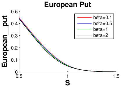
Stock varies to , strike price , , and
-red :
-blue :
-green :
-black :
4.2. ENVELOPE
In this section we study the range of node set of tree. We find an asymptotic envelope of boundary of tree.
Let which is the uppermost branch of tree. Then the recombination equation (5) becomes
Let different time scale and final time , then .
Consequently, letting go to zero, we obtain the envelope equation
| (7) | ||||
We find easily the solution of the envelope equation (7):


-blue : ode-solution envelope
-red : binomial tree envelope under the situation and , , , .
(a), (b)
We compare the envelope of binomial tree with the analytic envelope. Figure 5 gives a plot of the envelope when , and , , , . The envelopes of binomial trees follow the asymptotic solutions. There are two graph in each figure. One(-red) is binomial tree envelope, the other(-blue) is the solution to the envelope equation (7). We see that two curves agree well.
5. PRICING AMERICAN PUT OPTION UNDER CEV MODEL
American put option gives its holder the right (but not the obligation) to sell to the writer a prescribed asset for a prescribed price at any time between the start date and a prescribed expiry date in the future. American option differs from European option by the early exercise possibility. American option can be exercised at any time between the start date and the expiry date unlike European option which can only be exercised at maturity. Unfortunately, there is no analytic solution to the American option problem in general. It turns out that the binomial tree method can be used to value American put option. At each node we calculate the value of the option as a function of the next period prices. In chapter , the asset prices in the binomial model under the CEV diffusion are determined. If the put option is held until its maturity date , then
| (8) |
Here, , and is an exercise price. We work backward through the tree. If the option is retained, then is . However, exercising the option would produce . Hence choosing the best of the two possibilities leads to the relation.
| (9) |
Then we compute the time zero option value.

-, , and as stock price varies to
-red :
-blue :
-green :
-black :
Note , , denotes current stock price, strike price, time to maturity, respectively.
In Figure 6, we present numerical value for an American put, computed by the recombining binomial tree method with , , and as stock price varies to . Observe that American put option value is increasing as is decreasing like European put option value.
In figure 7, we also compare the probability distribution function of the recombining tree solution and the probability distribution of analytic solution
when .

6. CONCLUSION
In this paper, we discuss the pricing of American put option when the underlying stock follows Constant Elasticity of Variance (CEV) process. We constructed a recombining binomial tree to emulate CEV process. So we can apply it to pricing American put option, effectively. We tried to show the convergence of binomial tree method by comparing the European put option value between analytic solution and binomial tree. Our numerical results shows a good convergence. The binomial tree constructed in this paper has the advantage of being a most natural and simplest because it exactly recombines and has linear complexity for CEV model. It is our guess that our idea can be applied to different stochastic processes if we can derive Black-Scholes type partial differential equation.
References
- [1] S. BECKERS, The Constant Elasticity of Variance Model and Its Implications For Option Pricing , J. Finance, Vol. 35, No. 3(Jun., 1980), pp.661-673.
- [2] F. Black and M. Scholes, The pricing of options and corporate liabilities, The Journal of Political Economy, 81 (1973), 637-659.
- [3] J. Cox, Notes on Option Pricing I: Constant Elasticity of Diffusions, Unpublished draft, Stanford University, 1975.
- [4] J. Cox and S. Ross, The valuation of options for alternative stochastic processes, Journal of Financial Economics, 4 (1976), 145-166.
- [5] J. Cox and M. Rubinstein, Options markets, Prentice-Hall, 1985.
- [6] D. Nelson and K. Ramaswamy, Simple Binomial Processes as Diffusion Approximations in Financial Models, The Review of Financial Studies, Vol. 3, No. 3 (1990), 393-430
- [7] D. Emanuel and J. MacBeth, Further Results on the Constant Elasticity of Variance Call Option Pricing Model, Journal of Financial and Quantitative Analysis, 17 (1982), 533-554
- [8] R. Lu and Y. Hsu, Valuation of Standard Options under the Constant Elasticity of Variance Model, International Journal of Business and Economics, Vol. 4(2005), No. 2, 157-165
- [9] B. Peng and F. Peng, Pricing Arithmetic Options under the CEV process, J. Econ. Finance Adm. Sci., 15(19) (2010).
- [10] M. Schroder, Computing the constant elasticity of variance option pricing formula, J. Finance, 44 (1989), 211-219.
- [11] Tomer Neu-Ner, An Effective Binomial Tree Algorithm for the CEV Model. Technical report, School of Computational and Applied Mathematics, University of the Witwatersrand, November 2005.
- [12] H. Wong, Closed Form solution for Dynamic Fund Protection under CEV,