跳到论文正文
W Papers独立论文阅读器 arXiv:1410.5697 论文正文 计算阅读时间 · 0%
引用这篇论文根据当前论文元数据生成,正式投稿前建议核对。


License: arXiv.org perpetual non-exclusive license
arXiv:1410.5697v1 [cs.NI] 21 Oct 2014

Dynamic Optimization For Heterogeneous Powered Wireless Multimedia Sensor Networks With Correlated Sources and Network Coding

Abstract

The energy consumption in wireless multimedia sensor networks (WMSN) is much greater than that in traditional wireless sensor networks. Thus, it is a huge challenge to remain the perpetual operation for WMSN. In this paper, we propose a new heterogeneous energy supply model for WMSN through the coexistence of renewable energy and electricity grid. We address to cross-layer optimization for the multiple multicast with distributed source coding and intra-session network coding in heterogeneous powered wireless multimedia sensor networks (HPWMSN) with correlated sources. The aim is to achieve the optimal reconstruct distortion at sinks and the minimal cost of purchasing electricity from electricity grid. Based on the Lyapunov drift-plus-penalty with perturbation technique and dual decomposition technique, we propose a fully distributed dynamic cross-layer algorithm, including multicast routing, source rate control, network coding, session scheduling and energy management, only requiring knowledge of the instantaneous system state. The explicit trade-off between the optimization objective and queue backlog is theoretically proven. Finally, the simulation results verify the theoretic claims.

Index Terms: 
Wireless multimedia sensor networks, heterogeneous energy, cross-layer optimization, Lyapunov optimization, network coding, distributed source coding.

I Introduction

Wireless Multimedia Sensor Networks (WMSN) are composed of a large number of heterogeneous multimedia sensors, interconnected through wireless medium to capture video and audio streams, still images, and scalar sensor data, and transmits them to the sink(s) through the wireless manner. WMSN has a lot of potential new applications, for example, multimedia surveillance, traffic avoidance and control, health monitoring, environment monitoring, automated manufacturing processes, and industrial process control [1].

Similar to wireless sensor networks (WSN), the sensor nodes in WMSN are traditionally battery-operated, where the battery is usually limited and non-rechargeable. As the multimedia applications in WMSN require high transmission rate and extensive processing, the energy consumption of WMSN is much greater than that of WSN. Moreover, the sensors may be placed in remote and dangerous areas, the replacement of sensors is unrealistic and impossible. Hence, the network lifetime is an important issue for the operation of the most applications in WMSN, and an efficient power management should be proposed to extend the network lifetime. Recently, a large number of works focus on the energy efficiency for WMSN with the limited battery capacity [2][3]. Although the energy efficiency techniques increases the sensor’s lifetime, the network lifetime still has an upper bound due to the limited battery capacity. In order to solve this problem, the renewable energy technique is applied to power the sensors via solar panels or wind-powered generators [4]. However, the renewable energy technique exits some shortcoming, such as low recharging rate and time-varying profile of energy replenishment process, which can not guarantee to provide the perpetual operation for WMSN. As the electricity grid can provide persistent power input, the coexistence of renewable energy and electricity grid, called Heterogeneous Power (HP) is expected to achieve the infinite network lifetime[5].

Since the sensors in MWSN are always densely deployed in the most application scenarios, and the sensors generally have large monitoring range. For example, the nearby camera sensors’s monitoring range may be overlapped, and the multimedia information flows generated by them have a certain degree of spatial correlation and redundancy [6]. By removing the correlation and redundancy of the multimedia data, the amount of data transmitted in the network can be reduced, thereby reducing the energy consumption and improving the energy efficiency for MWSN. Distributed source coding (DSC) is one of the techniques that can remove the correlation and redundancy of multiple correlated sources, without communication between the sources. By modeling the correlation between multiple sources at the decoder side, DSC is able to shift the computation burden in sources to the joint decoder [7][8]. Thus, DSC provides appropriate frameworks for WMSN with complexity-constrained sensors and powerful sink(s). It is more important to use DSC in HPWMSN, since DSC enables multiple correlated sources to trade energy resources among them.

Network coding (NC) can combine various traffic flows or packets into a single packet in the intermediate node via simple algebraic operations, and then forwards it through one or more outgoing links[9]. Thus, NC has the potential of achieving substantial throughput and power efficiency gains in wireless networks. NC applied in WMSN can save a lot of energy consumption, and then prolong the lifetime of WMSN.

In this paper, we address a discrete-time stochastic cross-layer optimization problem with joint DSC and NC for HPWMSN to achieve the high energy efficiency and the desirable network performce. The key contribution are summarized as follows:

  • •

    Since most multimedia applications in WMSN require extensive data processing, we propose the overall energy consumption model to include multiple energy consumptions due to data processing, transmission and reception. In order to obtain potentially infinite lifetime, we propose the new energy heterogenous supply model through the coexistence of renewable energy and electricity grid. Sensors in WMSN can be powered by renewable energy, or electricity grid or both.

  • •

    We address to cross-layer optimization for the multiple multicast with DSC and NC in HPWMSN with correlated sources. We formulate a discrete-time stochastic cross-layer optimization problem with the goal of minimizing the time-average utility of reconstruct distortion at sinks and minimizing the cost of purchasing energy from electricity grid subject to network strong stability, link capacity, and data/energy availability constraints. This will involves all the layer of the network, such as the transmission layer, the network layer, especially the physical layer and medium access layer.

  • •

    Based the Lyapunov drift-plus-penalty with perturbation technique, we transfer the stochastic optimization problem into a deterministic optimization problem. By Lagrange dual decomposition, the problem is decoupled into five subproblems, including energy harvesting and battery charging/discharging problem, source rate control problem, distortion control problem, information/physical flow rate and power control problem, and session scheduling. Finally, a fully distributed iterative algorithm is designed.

  • •

    We analyze the performance of the proposed distributed algorithm, and show that a control parameter VV enables an explicit trade-off between the average objective value and queue backlog. Specifically, our algorithm can achieve a time average objective value that is within 𝒪⁡(1/V){\cal{O}}(1/V) of the optimal objective for any V>0V>0, while ensuring that the average queue backlog is 𝒪⁡(V){\cal{O}}(V). Finally, the simulation results verify the theoretic claims.

Throughout this paper, we use the following notations. We denote the probability Pr(A)(A) of an event AA. For a random variable XX, 𝔼⁡[X]\mathbb{E}[X] represents its expected value, 𝔼⁡[X|A]\mathbb{E}[X|{A}] represents its expected value conditioned on event AA. 1A\textbf{1}_{A} is the indicator function for an event AA, it is 1 if AA occurs and is 0 otherwise. [x]+=max⁡(x,0){{{[x]}^{+}}=\max(x,0)}.

The remainder of the paper is organized as follows. The related works are given in Section II. In Section III, we give the system model and problem formulation. In Section IV, we present the distributed cross-layer optimization algorithm. In Section V, we present the performance analysis of our proposed algorithm. Simulation results are given in Section VI. Concluding remarks are provided in Section VI.

II Related Works

II-A Distributed Source Coding

Using Slepian-Wolf model and a joint entropy coding model, Cristescu et al. in [10] propose a minimum cost of data transmission optimization problem in WSNs, where the sources are spatially correlated. Wang et al. in [11] propose a methodology for cross-layer optimization between routing and DSC in WSNs. In order to meet the data transmission latency and QoS requirements, Khoshroo et al. in [12] jointly consider the resource allocation, channel coding, and DSC. Cheng et al. in [13] proposed a hierarchical DSC coding scheme to completely remove inter-node data correlation and redundancy. Wang et al. in [14] jointly consider the optimization of Slepian-Wolf (SW) source coding and transmission rates to obtain the maximum source rate over a Gaussian multiple access channel. However, these works do not consider the link capacity constraint, which may cause congestion and deteriorate the network performance. Hence, Yuen et al. in [15] introduce the fixed link capacity constraint. They propose a distributed algorithm of joint rate allocation and transmission structure in WSN with correlated data. In practice, the link capacity depends on the power allocated to the link and the channel state. Ramamoorthy in [16] introduce the unfixed link capacity constraints, and consider a minimum cost optimization problem in WSN with multiple correlated sources. He et al. in [17] firstly focus on the network lifetime maximization that jointly considers routing, power control, and link-layer random access.

As far as we know, almost all works usually ignore the energy consumption of the data processing. However, in some applications, the energy consumption of data processing may be comparable to the energy consumption of data transmission. Hence, Tapparello et al. in [18] consider the joint energy allocation for communication module and processing module together in the multihop WSN scenario. They show that through applying DSC, the sensor with sufficient energy can ease the transmission requirements of correlated data on nearby node with low energy. This characteristic of DSC is very suitable for energy-harvesting networks. In [19], Stankovic et al. in [19] apply DSC to improve the network performance, consider the multimedia multicast over heterogeneous wireless-wireline networks, and propose a network-aware cross-layer optimization problem. In [8], Puri et al. apply distributed video coding to model the correlation between multiple sources at the decoder side together with channel codes. To the end, the encoder is simple, and the computational complexity is shifted to the decoder. Hence DSC is a promising technique for WMSN.

II-B Network Coding

The network coding techniques have been widely used in WSN. Chachulski et al. [20] exploit the broadcast nature of wireless transmission and propose a random network coding scheme. Li et al. in [21] consider multirate multicast with network coding over wireless video networks, to optimize the video quality and network performance. Lin et al. in [22] propose an approximate optimization scheme to jointly optimize the link scheduling, rate control, and flow allocation problems for multicast with intraflow network coding in multirate multichannel wireless mesh networks. Ho et al. [23] design a random linear network coding (RLNC) for wireless transmission. Chen et al. in [24] study the multicast flow control based network coding for wired networks and wireless networks. Rajawat et al. in [25] consider the random network coding for slotted wireless multihop networks. These works show that NC can obtain throughput gain and save a lot of energy and thus prolong the network lifetime. However, these works usually assume the data transmission over link is free of interference, which weakens the applicability of NC technique. Hence, some works address to NC in interference-limited networks. Xi et al. in [27] propose a framework for the minimum-cost optimization problem in interference-limited wireless networks, and jointly consider the power allocation, network coding and multicast. NC and DSC are jointly considered in [28] and [29]. Given a time-varying networks, Ho et al. in [28] propose a dynamic algorithms for the problem of multiple multicast sessions with intra-session network coding. [29] jointly consider the adaptive DSC, channel coding, NC and power control with QoS constraint for Co-Channel Interference (CCI)-limited wireless networks. However, they do not take the energy constraint into consideration, which is one of the most important constraint in WMSN.

III SYSTEM MODEL

We consider a general interconnected multi-hop WSN that operates over time slots t∈𝒯={0,1,2,…}t\in{\cal T}=\left\{{0,1,2,\ldots}\right\}. WSN is modeled by a direct graph 𝒢={𝒩,ℒ}{\cal G}=\left\{{{\cal N},{\cal L}}\right\}. 𝒩=𝒩H∪𝒩G∪𝒩M={1,2,3,…,N}{\cal N}={{\cal N}_{H}}\cup{{\cal N}_{G}}\cup{{\cal N}_{M}}=\left\{{1,2,3,\ldots,N}\right\} denotes the set of sensor nodes in the network, 𝒩H{\cal N}_{H} is the set of EH nodes powered by renewable energy, 𝒩G{\cal N}_{G} is the set of EG nodes powered by electricity grid, and 𝒩M{\cal N}_{M} is the set of ME nodes powered by both renewable energy and electricity grid, respectively. 𝒩s={1,2,…,Ns}⊂𝒩{\cal N}_{s}=\{1,2,\ldots,N_{s}\}\subset{\cal N} denotes the set of all source nodes which measure the information source(s), therein, we note that the sources are continuous and correlated. 𝒩d={1,2,…,Nd}⊂𝒩{\cal N}_{d}=\{1,2,\ldots,N_{d}\}\subset{\cal N} denotes the set of all sink nodes. Let ℱ={1,2,…,F}{\cal F}=\{1,2,\ldots,F\} denote the set of sessions in the network, and we assume the sessions are multicast, i.e., for ∀f∈ℱ\forall f\in{\cal F}, the session ff has at least one source and one sink. Therefore, we define 𝒩sf={1,2,3,…,Nsf}{\cal N}_{s}^{f}=\left\{{1,2,3,\ldots,N_{s}^{f}}\right\} and 𝒩df={1,2,3,…,Ndf}{\cal N}_{d}^{f}=\left\{{1,2,3,\ldots,N_{d}^{f}}\right\} as the set of session f′f^{\prime}s sources and sinks, respectively, 𝒩sf⊂𝒩s{\cal N}_{s}^{f}\subset{{\cal N}_{s}}, 𝒩sd⊂𝒩d{\cal N}_{s}^{d}\subset{{\cal N}_{d}}. The source node transmits the data to the corresponding sink node through multi-hop routing. We use 𝒪⁡(n){\cal O}\left(n\right) to denote the set of nodes mm with (n,b)∈ℒ(n,b)\in\cal L, and ℐ⁡(n){\cal I}\left(n\right) to denote the set of nodes aa with (a,n)∈ℒ(a,n)\in\cal L. ℒ={(n,b),n,b∈𝒩}​b∈𝒪⁡(n){\cal L}{\rm{=}}\left\{{(n,b),n,b\in{\cal N}}\right\}\,b\in{\cal O}\left(n\right) represents the set of communication links.

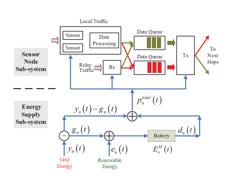
Fig. 1 describes the composition of a single node system, which is divided into two sub-systems, i.e., sensor node sub-system and energy supply sub-system. Sensor node sub-system includes data sensing/processing and data transmission/receiption. Their energy consumption is given in the subsection III-D. The energy supply sub-system is detailed described in the subsection III-E.
Refer to caption
Fig. 1: Node Composition.

III-A Network and Coding Model

In our network, in order to achieve the optimal throughout when transmit multiple multicast sessions, we apply the network coding technology. Note that the sink nodes only receive fractional sessions, combing different sessions together brings difficulty for data reconstruction, hence, we assume the network coding is limited within each session.

Let xn​bf​(t)x_{{nb}}^{f}\left(t\right) denote the physical flow rate of the session ff over link (n,b)\left({n,b}\right), and x~n​bf​s​d​(t)\tilde{x}_{nb}^{fsd}(t) denote the information flow rate of the session ff over link (n,b)\left({n,b}\right) from source s∈𝒩sfs\in{\cal N}_{s}^{f} to sink d∈𝒩dfd\in{\cal N}_{d}^{f}, where b∈𝒪⁡(n)b\in{\cal O}\left(n\right). Via network coding, the flows for different destinations of a multicast session can be coded together so that they can share the network capacity, while the actual physical flow over each link need only to be the maximum of the individual destinations’ flows, i.e.,

x~n​bf​s​d​(t)≤xn​bf​(t),f∈ℱ,s∈𝒩sf,d∈𝒩df,b∈𝒪⁡(n)\tilde{x}_{nb}^{fsd}\left(t\right)\leq x_{nb}^{f}\left(t\right),\;f\in{\cal F},\;s\in{\cal N}_{s}^{f},\;d\in{\cal N}_{d}^{f},\;b\in{\cal O}\left(n\right) (1)

III-B Distributed Lossy Coding

For continuous sources, we consider the lossy source coding which allows a reconstruction distortion. In our model, the distributed lossy coding can be described as the follows.

At every time slot tt, for each session ff, the node n∈𝒩sfn\in{\cal N}_{s}^{f} measures data from the environment and compresses it before transmission. We assume the node n∈𝒩sfn\in{\cal N}_{s}^{f} multicasts data to all the sinks of session ff at rate rnf​(t)r_{n}^{f}(t) with distortion Dnf​(t){D_{n}^{f}\left(t\right)}. Consider any subset ∀𝒩¯sf⊆𝒩sf\forall{\cal\underline{N}}_{s}^{f}\subseteq{\cal N}_{s}^{f}, for each node n∈𝒩¯sfn\in{\cal\underline{N}}_{s}^{f} ,we have:

∑n∈𝒩¯sfrnf​(t)≥H⁡(𝒩¯sf|𝒩sf−𝒩¯sf)−log⁡((2​π​e)|𝒩¯sf|​∏n∈𝒩¯sfDnf​(t))\sum\limits_{n\in{\cal\underline{N}}_{s}^{f}}{r_{n}^{f}}(t)\geq H\left({{\cal\underline{N}}_{s}^{f}|{\cal N}_{s}^{f}-{\cal\underline{N}}_{s}^{f}}\right)-\log((2{\pi}e)^{|{\cal\underline{N}}_{s}^{f}|}\prod\limits_{n\in{\cal\underline{N}}_{s}^{f}}{D_{n}^{f}\left(t\right)}) (2)

where H⁡(𝒩¯sf|𝒩sf−𝒩¯sf)H\left({{\cal\underline{N}}_{s}^{f}|{\cal N}_{s}^{f}-{\cal\underline{N}}_{s}^{f}}\right) represents the entropy of 𝒩¯sf{\cal\underline{N}}_{s}^{f} conditioned on 𝒩sf−𝒩¯sf{\cal N}_{s}^{f}-{\cal\underline{N}}_{s}^{f}.

We also assume that

0≤rnf​(t)≤Rmax,∀f∈ℱ,n∈𝒩sf0\leq{r_{n}^{f}}(t)\leq R_{\max}{\rm{,}}\forall f\in{\cal F},n\in{\cal N}_{s}^{f} (3)

and

Dmin≤Dnf​(t)≤Dmax,∀f∈ℱ,n∈𝒩sfD_{\min}\leq{D_{n}^{f}}(t)\leq D_{\max}{\rm{,}}\forall f\in{\cal F},n\in{\cal N}_{s}^{f} (4)

III-C Random Access and Data Transmission

We assume that the links in the network may interfere with each other when they transmit data simultaneously, we also assume each node cannot transmit or receive at the same time, and define qn​(t){q_{n}}\left(t\right) as the transmission probability of node nn at slot tt, with

0≤qn​(t)≤1,∀n∈𝒩.0\leq{q_{n}}\left(t\right)\leq 1,\forall n\in{\cal N}. (5)

When node nn is selected to transmits data at slot tt, the probability of choosing outgoing link (n,b),b∈𝒪⁡(n)\left({n,b}\right),b\in{\cal O}\left(n\right) is qn​b​(t){q_{nb}}\left(t\right), with ∑b∈𝒪⁡(n)qn​b​(t)=qn​(t)\sum\limits_{b\in{\cal O}\left(n\right)}{{q_{nb}}\left(t\right)}={q_{n}}\left(t\right) .

Then, we introduce the transmission probability matrix ȷ(t)={qn​b(t),(n,b)∈ℒ|0≤qn​b(t)≤1}{\bm{\jmath}}\left(t\right)=\left\{{{q_{nb}}\left(t\right),\left({n,b}\right)\in{\cal L}|0\leq{q_{nb}}\left(t\right)\leq 1}\right\} . Summary, the link (n,b)(n,b) can transmit data successfully at time slot tt with probability

αn​b​(t)=qn​b​(t)​(∏a∈ℐ⁡(n)(1−qa​n​(t)))⏟The​probabilityof​no​acceptionof​n​(1−∑c∈𝒪⁡(b)qb​c​(t)⏟The​probability​ofno​transmissionof​b){\alpha_{nb}}\left(t\right)={q_{nb}}\left(t\right)\underbrace{(\prod\limits_{a\in{\cal I}\left(n\right)}{(1-{q_{an}}\left(t\right)}))}_{\scriptstyle\;\rm{The}\,\rm{probability}\;\hfill\atop{\scriptstyle\;\rm{of}\,\rm{no}\,\,\rm{acception}\hfill\atop\scriptstyle\;\;\;\hskip 7.97224pt\rm{of}\,\rm{n}\hfill}}(\underbrace{1-\sum\limits_{c\in{\cal O}\left(b\right)}{{q_{bc}}\left(t\right)}}_{\scriptstyle\;\rm{The}\,\rm{probability}\;\rm{of}\,\hfill\atop{\scriptstyle\;\rm{no}\,\,\rm{transmission}\hfill\atop\scriptstyle\;\;\;\hskip 7.97224pt\rm{of}\,\rm{b}\hfill}}),

We define 𝑷⁡(t)=(pn​bT​(t),(n,b)∈ℒ){\bm{P}}\left(t\right){\rm{=}}\left({{p_{nb}^{T}}\left(t\right),\left({n,b}\right)\in{\cal L}}\right) as the power allocation matrix for data transmission at slot tt, where pn​bT​(t){p_{nb}^{T}}(t) is the power allocated to link (n,b)\left({n,b}\right), and each node nn satisfies

0≤∑b∈𝒪⁡(n)pn​bT​(t)≤Pnmax,0\leq\sum\limits_{b\in{\cal O}\left(n\right)}{{p_{nb}^{T}}(t)}\leq{P_{n}^{\max}}, (6)

Next, we use γn​b​(t){\gamma_{nb}}(t) to denote the signal to interference plus noise ratio (SINR) of link (n,b)\left({n,b}\right), which can be calculated by the following:

γn​b​(t)=Sn​bC​(t)​pn​bT​(t)Nn​b+∑a∈ℐn,b∑(a,c)∈ℒSa​bC​(t)​pa​cT​(t)​qa​c​(t),{\gamma_{nb}}(t)=\frac{{{S_{nb}^{C}(t)}{p_{nb}^{T}}\left(t\right)}}{{{N_{nb}}+\sum\limits_{a\in{\cal I}_{n,b}}\sum\limits_{\left({a,c}\right)\in{\cal L}}{{S_{ab}^{C}(t)}{p_{ac}^{T}}\left(t\right){q_{ac}}\left(t\right)}}}, (7)

where ℐn,b{\cal I}_{n,b} represents the set of nodes whose transmission can interfere the transmission over link (n,b)(n,b), Sn​bC​(t){S_{nb}^{C}(t)} represents the link fading coefficient from nn to bb, and Nn​b{N_{nb}} represents the noise which is assumed to be constant.We assume that Sn​bC​(t){S_{nb}^{C}}(t) may be time varying and i.i.d. at every slot. Denote 𝑺C​(t)={Sn​bC​(t),(n,b)∈ℒ}{\bm{S}}^{C}(t)=\{{S}_{nb}^{C}(t),(n,b)\in\cal L\} as the network channel state matrix, taking non-negative values from a finite but arbitrarily large set 𝒮C{\cal S}^{C}.

The link capacity is defined as the following:

Cn​b​(t)=B​W​αn​b​(t)​log⁡(γn​b​(t)){C_{nb}}\left(t\right)=BW{\alpha_{nb}(t)}\log\left({{\gamma_{nb}(t)}}\right) (8)

where B​WBW is the bandwidth.

Because of the total rates of all sessions cannot exceed the link capacity, so, the following constraints must be met:

0≤∑f∈ℱxn​bf​(t)≤Cn​b​(t),∀n∈𝒩,∀b∈𝒪⁡(n)0\leq\sum\limits_{f\in{\cal F}}{x_{{nb}}^{f}\left(t\right)}\leq C_{nb}(t),\forall n\in{\cal N},\forall b\in{\cal O}\left(n\right) (9)

Without loss of generality, we assume that for all time over all links under any power allocation matrix and any channel state, there exists some finite constant XmaxX_{\max} such that

0≤∑f∈ℱxn​bf​(t)≤Xmax0\leq\sum\limits_{f\in{\cal F}}{x_{{nb}}^{f}\left(t\right)}\leq X_{\max} (10)

III-D Energy Consumption Model

The energy consumption model is divided into three parts:data sensening/processing, data transmission and data reception. Therein, we define P~fS{\tilde{P}_{f}^{S}} and P~nR{\tilde{P}_{n}^{R}} as the cost of per data sensing and reception, respectively.

When node n∈𝒩sfn\in{\cal N}_{s}^{f} achieves the compressed data rate at rnf​(t)r_{n}^{f}(t) , we assume the energy consumed is P~fS​rnf​(t)\tilde{P}_{f}^{S}r_{n}^{f}(t), which is linear. When node nn receives session f∈ℱf\in\cal F from its neighbor node a∈ℐna\in{\cal I}_{n} at rate xa​nf​(t)x_{{an}}^{f}\left(t\right), the energy required is PnR​xa​nf​(t)P_{n}^{R}x_{{an}}^{f}\left(t\right). Above all, the total energy consumption pnT​o​t​a​l​(t)p_{n}^{Total}\left(t\right) of node nn at slot tt is:

pnT​o​t​a​l​(t)\displaystyle p_{n}^{Total}\left(t\right) =Δ\displaystyle\mathrel{\mathop{\kern 0.0pt=}\limits^{\Delta}} ∑f∈ℱ1n∈𝒩sf​P~fS​rnf​(t)+∑b∈𝒪⁡(n)pn​bT​(t)\displaystyle\sum\limits_{f\in{\cal F}}\textbf{1}_{n\in{{\cal N}_{s}^{f}}}{\tilde{P}_{f}^{S}}{r_{n}^{f}}\left(t\right)+\sum\limits_{b\in{\cal O}\left(n\right)}{p_{nb}^{T}\left(t\right)} (11)
+\displaystyle+ P~nR​∑a∈ℐ⁡(n)∑f∈ℱxa​nf​(t)\displaystyle\tilde{P}_{n}^{R}\sum\limits_{a\in{\cal I}\left(n\right)}{\sum\limits_{f\in{\cal F}}{x_{{an}}^{f}\left(t\right)}}

III-E Energy Supply Model

First, we describe the energy supply model of ME node shown in Fig.1. Each ME node is equipped with a battery. As depicted in Fig.1, the harvested energy en​(t)e_{n}(t) at time tt for ME node nn is stored in the battery. On the other hand, the energy supplied by the electricity grid at time tt for ME node nn is denoted with yn​(t)y_{n}(t). Some of this grid energy is used to charge the battery at a charging rate gn​(t)g_{n}(t), while the remaining energy yn​(t)−gn​(t)y_{n}(t)-g_{n}(t) is used to supply the operation of ME node nn. In addition, some energy from the battery is discharged at a discharging rate dn​(t)d_{n}(t) to supplement the energy drawn from the electricity grid so as to meet the energy demand of the node. Thus, the total energy consumption pnT​o​t​a​l​(t)p_{n}^{Total}\left(t\right) of a ME node nn at slot tt is determined by the energy supplied by the electricity grid, and the energy discharged from the battery, therefore expressed as

pnT​o​t​a​l​(t)=yn​(t)−gn​(t)+dn​(t)p_{n}^{Total}\left(t\right)={y_{n}}\left(t\right)-{g_{n}}\left(t\right)+{d_{n}}\left(t\right)

which is equivalent to

yn​(t)=Δgn​(t)−dn​(t)+pnT​o​t​a​l​(t),∀n∈𝒩G∪𝒩M.{y_{n}}\left(t\right)\mathrel{\mathop{\kern 0.0pt=}\limits^{\Delta}}{g_{n}}\left(t\right)-{d_{n}}\left(t\right)+p_{n}^{Total}\left(t\right),\forall n\in{\mathcal{N}}_{G}\cup{\mathcal{N}}_{M}. (12)

III-E1 Energy queue

We assume each ME-node nn knows its own current energy availability EnM​(t){{E_{n}^{M}}}\left(t\right)\; denoting the energy queue size for n∈𝒩M\,n\in{\cal N}_{M}\, at time slot tt. We define 𝑬M​(t)=(EnM​(t),n∈𝒩M){\bm{E}}_{M}\left(t\right)=\left({{{E_{n}^{M}}}\left(t\right),n\in{\cal N}_{M}}\right) over time slots t∈𝒯t\in\cal T as the vector of the energy queue sizes. For ME node nn, the energy queuing dynamic equation is

EnM​(t+1)=EnM​(t)+en​(t)+gn​(t)−dn​(t)E_{n}^{M}\left({t+1}\right)=E_{n}^{M}\left(t\right)+{{e_{n}}\left(t\right)+{g_{n}}\left(t\right)}-{d_{n}}\left(t\right) (13)

with EnM​(0)=0E_{n}^{M}\left(0\right)=0. In any time slot tt, the total energy consumption at ME node nn must satisfy the following energy-availability constraint:

EnM​(t)≥dn​(t),∀n∈𝒩M.{{E_{n}^{M}}}\left(t\right)\geq{d_{n}}\left(t\right),\;\;\forall n\in{{\cal N}_{M}}. (14)

III-E2 Two special cases

In fact, both EH node and EG node are two special cases of ME node.

For EH node, yn​(t)=0,gn​(t)=0{y_{n}}\left(t\right)=0,\;{g_{n}}\left(t\right)=0, and so pnT​o​t​a​l​(t)=dn​(t)p_{n}^{Total}\left(t\right)={d_{n}}\left(t\right). Thus, the energy queuing dynamic equation at EH node nn is changed from (13) into:

EnH​(t+1)=EnH​(t)+en​(t)−pnT​o​t​a​l​(t),n∈𝒩H,{{E_{n}^{H}}}\left({t+1}\right)={{E_{n}^{H}}}\left(t\right)+{e_{n}}\left(t\right)-p_{n}^{Total}\left(t\right),\;\;n\in{{\cal N}_{H}}, (15)

with EnH​(0)=0E_{n}^{H}\left(0\right)=0. The energy-availability constraint is changed from (14) into:

EnH​(t)≥pnT​o​t​a​l​(t),∀n∈𝒩H.{{E_{n}^{H}}}\left(t\right)\geq p_{n}^{Total}\left(t\right),\;\;\forall n\in{{\cal N}_{H}}. (16)

For EG node, en​(t)=0{e_{n}}\left(t\right)=0. Thus, the energy queuing dynamic equation at EG node nn is changed from (13) into:

EnG​(t+1)=EnG​(t)+gn​(t)−dn​(t),n∈𝒩G{{E_{n}^{G}}}\left({t+1}\right)={{E_{n}^{G}}}\left(t\right)+{g_{n}}\left(t\right)-{d_{n}}\left(t\right),\;\;n\in{{\cal N}_{G}} (17)

with EnG​(0)=0E_{n}^{G}\left(0\right)=0. The energy-availability constraint is changed from (14) into:

EnG​(t)≥dn​(t),∀n∈𝒩G.{{E_{n}^{G}}}\left(t\right)\geq{d_{n}}\left(t\right),\;\;\forall n\in{{\cal N}_{G}}. (18)

We define 𝑬H​(t)=(EnH​(t),n∈𝒩H){\bm{E}}_{H}\left(t\right)=\left({{{E_{n}^{H}}}\left(t\right),n\in{\cal N}_{H}}\right) and 𝑬G​(t)=(EnG​(t),n∈𝒩G){\bm{E}}_{G}\left(t\right)=\left({{{E_{n}^{G}}}\left(t\right),n\in{\cal N}_{G}}\right) over time slots t∈𝒯t\in{\cal T} as the vector of the energy queue sizes for all EH nodes and that for all EG nodes, respectively.

III-E3 Some constraints

We assume the available amount of harvesting energy at slot tt is hn​(t){h_{n}}\left(t\right) with hn​(t)≤hmax{h_{n}}\left(t\right)\leq{h_{\max}} for all tt. The amount of actually harvested energy en​(t){e_{n}}\left(t\right) at slot tt, should satisfy

0≤en​(t)≤hn​(t),∀n∈𝒩H∪𝒩M,0\leq{e_{n}}\left(t\right)\leq{h_{n}}(t),\forall n\in{{{\cal N}_{H}}\cup{{\cal N}_{M}}}, (19)

where hn​(t){h_{n}}\left(t\right) is randomly varying over time slots in an i.i.d. fashion according to a potentially unknown distribution and taking non-negative values from a finite but arbitrarily large set 𝒮H{\cal S}^{H}. We define the harvestable energy vector 𝑺H​(t)=(hn​(t),n∈𝒩H∪𝒩M){{\bm{S}}^{H}}(t)=\left({{h_{n}}\left(t\right),n\in{{{\cal N}_{H}}\cup{{\cal N}_{M}}}}\right), called the harvestable energy state.

The charging rate gn​(t){g_{n}}\left(t\right)\; of the battery of node nn at slot tt should satisfy:

0≤gn​(t)≤gnmax,∀n∈𝒩G∪𝒩M,0\leq{g_{n}}\left(t\right)\leq g_{n}^{\max},\forall n\in{{{\cal N}_{G}}\cup{{\cal N}_{M}}}, (20)

with some finite gnmaxg_{n}^{\max}.

The discharging rate dn​(t){d_{n}}\left(t\right)\; of the battery of node nn at slot tt should satisfy:

0≤dn​(t)≤dnmax,∀n∈𝒩G∪𝒩M,0\leq{d_{n}}\left(t\right)\leq d_{n}^{\max},\forall n\in{{{\cal N}_{G}}\cup{{\cal N}_{M}}}, (21)

with some finite dnmaxd_{n}^{\max}.

the energy supplied by the electricity grid yn​(t){y_{n}}\left(t\right)\; of the node nn at slot tt should satisfy:

0≤yn​(t)≤ynmax,∀n∈𝒩G∪𝒩M,0\leq{y_{n}}\left(t\right)\leq y_{n}^{\max},\forall n\in{{{\cal N}_{G}}\cup{{\cal N}_{M}}}, (22)

with some finite ynmaxy_{n}^{\max}.

Moreover, at any time slot tt, we also assume the total energy volume stored in battery on node n∈𝒩Hn\in{\cal N}_{H} is limited by the weight perturbation θne​H\theta_{n}^{{eH}} introduced in section IV, the reason will be explained in Theorem 1, thus the following inequations must be satisfied

EnH​(t)+en​(t)≤θne​H,∀n∈𝒩H{{E_{n}^{H}}}(t)+{e_{n}}\left(t\right)\leq{\theta_{n}^{{eH}}},\forall n\in{{\cal N}_{H}} (23)

III-F Electricity Price Model

At time slot tt, the cost of purchasing one unit electricity from the electricity grid at node n∈𝒩G∪𝒩Mn\in{\mathcal{N}}_{G}\cup{\mathcal{N}}_{M} is characterized by the function PnG​(t)P_{n}^{G}(t), which may be with respect to the energy yn​(t)y_{n}(t) supplied by EG and the electricity price state variable SnG​(t)S_{n}^{G}(t). We assume SnG​(t)S_{n}^{G}(t) is an i.i.d. process and takes non-negative values from a finite but arbitrarily large set 𝒮G{\cal S}^{G}. Denote 𝑺G​(t)={SnG​(t),n∈𝒩G∪𝒩M}{\bm{S}}^{G}(t)=\{S_{n}^{G}(t),n\in{{{\cal N}_{G}}\cup{{\cal N}_{M}}}\} as the electricity price vector. Therein, we assume that PnG​(t)P_{n}^{G}(t) is a function of both SnG​(t)S_{n}^{G}(t) and yn​(t)y_{n}(t), i.e.,

PnG​(t)=PnG​(SnG​(t),yn​(t))P_{n}^{G}(t)=P_{n}^{G}(S_{n}^{G}(t),y_{n}(t))

Note that the dependence of PnG​(t)P_{n}^{G}(t) on SnG​(t)S_{n}^{G}(t) and yn​(t)y_{n}(t) is implicit for notational convenience in the sequel. For each SnG​(t)S_{n}^{G}(t), PnG​(t)P_{n}^{G}(t) is assumed to be a increasing and continuous convex function of yn​(t)y_{n}(t).

III-G Data Queue Model

For f∈ℱf\in{\cal F} at node nn, we use Qnf​s​d​(t){Q}_{n}^{fsd}\left(t\right)\; to denote the data backlog of the ff-th session from source s∈𝒩sfs\in{\cal N}_{s}^{f} to sink d∈𝒩dfd\in{\cal N}_{d}^{f} at slot tt. We define 𝑸⁡(t)=(Qnf​s​d​(t),n∈𝒩,f∈ℱ,s∈𝒩sf,d∈𝒩df){{\bm{Q}}}\left(t\right)=\left({{Q}_{n}^{fsd}\left(t\right),n\in{\cal N},f\in{\cal F},s\in{\cal N}_{s}^{f},d\in{\cal N}_{d}^{f}}\right) over time slots t∈𝒯t\in\cal T . Then, the data queuing dynamic equation at the network layer is

Qnf​s​d​(t+1)\displaystyle{Q}_{n}^{fsd}(t{\rm{+1}}) =\displaystyle= Qnf​s​d​(t)−∑b∈𝒪⁡(n)x~n​bf​s​d​(t)\displaystyle{Q}_{n}^{fsd}(t)-\sum\limits_{b\in{\cal O}\left(n\right)}{\tilde{x}_{{nb}}^{fsd}\left(t\right)} (24)
+\displaystyle+ ∑a∈ℐ⁡(n)x~a​nf​s​d​(t)+1f∈ℱn​rnf​(t).\displaystyle\sum\limits_{a\in{\cal I}\left(n\right)}{\tilde{x}_{{an}}^{fsd}\left(t\right)}+{\textbf{1}_{f\in{{\cal F}_{n}}}}{r_{n}^{f}}\left(t\right).

with Qnf​s​d​(0)=0{Q}_{n}^{fsd}\left(0\right)=0. Also, the following data-availability constraint at the network layer should be satisfied:

0\displaystyle 0 ≤∑b∈𝒪⁡(n)x~n​bf​s​d​(t)≤Qnf​s​d​(t),\displaystyle\leq\sum\limits_{b\in{\cal O}\left(n\right)}{\tilde{x}_{{nb}}^{fsd}\left(t\right)}\leq{{{Q}_{n}^{fsd}}}\left(t\right), (25)
∀n∈𝒩,f∈ℱ,s∈𝒩sf,d∈𝒩df.\displaystyle\forall n\in{{\cal N}},f\in{{\cal F}},s\in{\cal N}_{s}^{f},d\in{\cal N}_{d}^{f}.

To ensure the network is strongly stable, the following inequation must be satisfied:

limT→∞1T​∑t=0T−1∑n∈𝒩∑f∈ℱ∑s∈𝒩sf∑d∈𝒩df𝔼⁡{Qnf​s​d​(t)}<∞\mathop{\lim}\limits_{T\to\infty}\frac{1}{T}\sum\limits_{t=0}^{T-1}{\sum\limits_{n\in{\cal N}}{\sum\limits_{f\in{\cal F}}{\sum\limits_{s\in{\cal N}_{s}^{f}}{\sum\limits_{d\in{\cal N}_{d}^{f}}\mathbb{E}{\left\{{Q_{n}^{fsd}(t)}\right\}<\infty}}}}} (26)

III-H Optimization Problem

For each session ff, at each node n∈𝒩sfn\in{\cal N}_{s}^{f}, we assume the utility is Unf​(Dnf​(t)){U_{n}^{f}\left({D_{n}^{f}\left(t\right)}\right)} with the corresponding distortion Dnf​(t)D_{n}^{f}\left(t\right). We assume the Unf​(⋅){U_{n}^{f}\left(\cdot\right)} is decreasing and concave. So, our goal is to design a full distributed algorithm that achieves the optimal trade-off between the time-average utility of the distortion and the time-average cost of energy consumption in electricity grid subject to all of the constraints described above.

Mathematically, we will address the stochastic optimization problem P1 as follows:

maximize{𝝌⁡(t),t∈𝒯}\displaystyle\mathop{\mbox{maximize}}_{\{{\bm{\chi}}(t),t\in\cal T\}} O¯=limT→∞1T​∑t=0T−1𝔼⁡{O⁡(t)}\displaystyle\overline{O}=\mathop{\lim}\limits_{T\to\infty}\;\frac{1}{T}\sum\limits_{t=0}^{T-1}\mathbb{E}{\left\{{O\left(t\right)}\right\}} (27)
subject to (1)−(6),(9),(10),(12),(14),\displaystyle\eqref{networkcoding}-\eqref{energy constraint},\eqref{link_rate constraint},\eqref{Xmax},\eqref{EG_energysupply},\eqref{EMenergy_availability},
(16),(18),(19)−(23),(25),(26)\displaystyle\eqref{EHenergy_availability},\eqref{EGenergy_availability},\eqref{harvesting_decision}-\eqref{limitedcapacityeh},\eqref{Data_availability},\eqref{qstable}

with the queuing dynamics (13) for ∀n∈𝒩M\forall n\in{{\cal N}_{M}}, (15) for ∀n∈𝒩H\forall n\in{{\cal N}_{H}}, (17) for ∀n∈𝒩G\forall n\in{{\cal N}_{G}}, and (24) for ∀n∈𝒩,∀f∈ℱ,s∈𝒩sf,d∈𝒩df\forall n\in{\cal N},\forall f\in{\cal F},s\in{\cal N}_{s}^{f},d\in{\cal N}_{d}^{f}.

𝝌⁡(t)=Δ(𝒆⁡(t),𝒓⁡(t),𝑫⁡(t),𝒚⁡(t),𝒈⁡(t),𝒅⁡(t),𝒑T​(t),𝒙⁡(t),𝒙~​(t),𝒒⁡(t)){\bm{\chi}}(t)\mathrel{\mathop{\kern 0.0pt=}\limits^{\Delta}}({\bm{e}}(t),{\bm{r}}(t),{\bm{D}}(t),{\bm{y}}(t),{\bm{g}}(t),{\bm{d}}(t),{\bm{p}}^{T}(t),{\bm{x}}(t),\tilde{{\bm{x}}}(t),\\ {\bm{q}}(t)) is the set of the optimal variables of the problem P1, where 𝒆⁡(t){\bm{e}}(t), 𝒓⁡(t){\bm{r}}(t), 𝑫⁡(t){\bm{D}}(t), 𝒚⁡(t){\bm{y}}(t), 𝒈⁡(t){\bm{g}}(t), 𝒅⁡(t){\bm{d}}(t), 𝒑T​(t){\bm{p}}^{T}(t), 𝒙⁡(t){\bm{x}}(t) ,𝒙~​(t)\tilde{{\bm{x}}}(t), 𝒒⁡(t){\bm{q}}(t) are the vector of en​(t){e_{n}}(t), rnf​(t){r_{n}^{f}}(t), Dnf​(t){D_{n}^{f}}(t), yn​(t){y_{n}}(t), gn​(t){g_{n}}(t), dn​(t){d_{n}}(t), pnT​(t){p_{n}^{T}}(t), xn​bf​(t){x}_{nb}^{f}(t), x~n​bf​s​d​(t)\tilde{x}_{nb}^{fsd}(t), qn​b​(t)q_{nb}(t), respectively.

O⁡(t)\displaystyle O\left(t\right) =\displaystyle= ϖ1​∑f∈ℱ∑n∈𝒩sfUnf​(Dnf​(t))\displaystyle\varpi_{1}\sum\limits_{f\in{\cal F}}\sum\limits_{n\in{\cal N}_{s}^{f}}U_{n}^{f}(D_{n}^{f}(t))
−\displaystyle- (1−ϖ1)​ϖ2​∑n∈𝒩G∪𝒩MPnG​(t)​yn​(t)\displaystyle(1-\varpi_{1})\varpi_{2}\sum\limits_{n\in{{{\cal N}_{G}}\cup{{\cal N}_{M}}}}{P_{n}^{G}(t)}{y_{n}(t)}

IV Distributed Cross-layer Optimization Algorithm

In this section, we assume the rand access probabilities are known a prior, so we will only determine the energy harvesting, the energy purchasing and battery dischage/charge, energy allocation, routing and scheduling decisions.

We will propose a fully distributed algorithm which makes greedy decisions at each time slot without requiring any statistical knowledge of the harvestable energy states, of the electricity price states and of the channel states.

IV-A Lyapunov optimization

First, we introduce the weight perturbation 𝜽e​H=(θne​H,n∈𝒩H){{\bm{\theta}}^{{eH}}}=\left({\theta_{n}^{{eH}},n\in{{\cal N}_{H}}}\right), 𝜽e​M=(θne​M,n∈𝒩M){{\bm{\theta}}^{{eM}}}=\left({\theta_{n}^{{eM}},n\in{{\cal N}_{M}}}\right) and 𝜽e​G=(θne​G,n∈𝒩G){{\bm{\theta}}^{{eG}}}=\left({\theta_{n}^{{eG}},n\in{{\cal N}_{G}}}\right). Then we define the network state at time slot tt as
𝒁⁡(t)=Δ(𝑺C​(t),𝑺H​(t),𝑺G​(t),𝑸⁡(t),𝑬𝑴​(t),𝑬𝑯​(t),𝑬𝑮​(t)){\bm{Z}}(t)\mathrel{\mathop{\kern 0.0pt=}\limits^{\Delta}}({{\bm{S}}^{C}}(t),{{\bm{S}}^{H}}(t),{{\bm{S}}}^{G}(t),{\bm{Q}}(t),{\bm{E_{M}}}(t),{\bm{E_{H}}}(t),{\bm{E_{G}}}(t)). Define the Lyapunov function as

L⁡(t)\displaystyle{L}(t) =\displaystyle= 12​∑n∈𝒩∑f∈ℱ∑s∈𝒩sf∑d∈𝒩df(Qnf​s​d​(t))2\displaystyle\frac{1}{2}\sum\limits_{n\in{\cal N}}{\sum\limits_{f\in{\cal F}}\sum\limits_{s\in{\cal N}_{s}^{f}}\sum\limits_{d\in{\cal N}_{d}^{f}}{{{\left({{Q}_{n}^{fsd}(t)}\right)}^{2}}}} (28)
+\displaystyle+ 12​∑n∈𝒩H(EnH​(t)−θne​H)2\displaystyle\frac{1}{2}\sum\limits_{n\in{{\cal N}_{H}}}{{{\left({{{E_{n}^{H}}}\left(t\right)-\theta_{n}^{{eH}}}\right)}^{2}}}
+\displaystyle+ 12​∑n∈𝒩M(EnM​(t)−θne​M)2\displaystyle\frac{1}{2}\sum\limits_{n\in{{\cal N}_{M}}}{{{\left({{{E_{n}^{M}}}\left(t\right)-\theta_{n}^{{eM}}}\right)}^{2}}}
+\displaystyle+ 12​∑n∈𝒩G(EnG​(t)−θne​G)2\displaystyle\frac{1}{2}\sum\limits_{n\in{{\cal N}_{G}}}{{{\left({{{E_{n}^{G}}}\left(t\right)-\theta_{n}^{{eG}}}\right)}^{2}}}

Remark 3.1 From the above equation (28), we can see that when minimizing the Lyapunov function L⁡(t)L(t), we push the queue backlog towards the corresponding perturbed variable value. So, as long as we choose appropriate perturbed variables, the constraint (14), (16) and (18) will always be satisfied. The detailed proof will be given in the next section. Thus, we can get rid of this constraint in the sequel.

Now define the drift-plus-penalty as
ΔV​(t)=Δ𝔼⁡(L⁡(t+1)−L⁡(t)−V​O​(t)|𝒁⁡(t)){\Delta_{V}}\left(t\right)\mathrel{\mathop{\kern 0.0pt=}\limits^{\Delta}}\mathbb{E}\left(L(t+1)-L(t)-VO(t)|{\bm{Z}}(t)\right), where VV is a non-negative weight, which can be tuned to control O¯\overline{O} arbitrarily close to the optimum with a corresponding tradeoff in average queue size. Next, the upper bound of ΔV​(t){\Delta_{V}}\left(t\right) is given in

ΔV(t)≤B+𝔼(Δ^V(t)|𝒁(t)),{\Delta_{V}}\left(t\right)\leq B+\mathbb{E}\left({\hat{{\Delta}}_{V}}\left(t\right)\left|{{\bm{Z}}(t)}\right.\right), (29)

where Δ^V​(t){\hat{\Delta}_{V}}\left(t\right) is shown in (30),

Δ^V​(t)\displaystyle{\hat{{\Delta}}_{V}}\left(t\right) =\displaystyle= ∑n∈𝒩∑f∈ℱ∑s∈𝒩sf∑d∈𝒩dfQnf​s​d​(t)​(∑a∈ℐ⁡(n)x~a​nf​s​d​(t)+𝟏n=s​rsf​(t)−∑b∈𝒪⁡(n)x~n​bf​s​d​(t))\displaystyle\sum\limits_{n\in{\cal N}}{\sum\limits_{f\in{\cal F}}{\sum\limits_{s\in{\cal N}_{s}^{f}}{\sum\limits_{d\in{\cal N}_{d}^{f}}{Q_{n}^{fsd}(t)\left({\sum\limits_{a\in{\cal I}(n)}{\tilde{x}_{an}^{fsd}(t)}+{{\bm{1}}_{n=s}}r_{s}^{f}(t)-\sum\limits_{b\in{\cal O}(n)}{\tilde{x}_{nb}^{fsd}(t)}}\right)}}}} (30)
+\displaystyle+ ∑n∈𝒩H(EnH​(t)−θne​H)​(en​(t)−pnT​o​t​a​l​(t))\displaystyle{\sum\limits_{n\in{{\cal N}_{H}}}{\left({{{E_{n}^{H}}}\left(t\right)-\theta_{n}^{{eH}}}\right)\left({e_{n}}\left(t\right)-p_{n}^{Total}\left(t\right)\right)}}
+\displaystyle+ ∑n∈𝒩M(EnM​(t)−θne​M)​(en​(t)+gn​(t)−dn​(t))\displaystyle{\sum\limits_{n\in{{\cal N}_{M}}}{\left({{{E_{n}^{M}}}\left(t\right)-\theta_{n}^{{eM}}}\right)\left({e_{n}}\left(t\right)+{g_{n}}\left(t\right)-{d_{n}}\left(t\right)\right)}}
+\displaystyle+ ∑n∈𝒩G(EnG​(t)−θne​G)​(gn​(t)−dn​(t))\displaystyle{\sum\limits_{n\in{{\cal N}_{G}}}{\left({{{E_{n}^{G}}}\left(t\right)-\theta_{n}^{{eG}}}\right)\left({g_{n}}\left(t\right)-{d_{n}}\left(t\right)\right)}}
−\displaystyle- V⁡(ϖ1​∑f∈ℱ∑n∈𝒩sfUnf​(Dnf​(t))−(1−ϖ1)​ϖ2​∑n∈𝒩G∪𝒩MPnG​(t)​yn​(t))\displaystyle V\left({\varpi_{1}\sum\limits_{f\in{\cal F}}{\sum\limits_{n\in{\cal N}_{s}^{f}}{U_{n}^{f}\left({D_{n}^{f}\left(t\right)}\right)}-(1-\varpi_{1})\varpi_{2}\sum\limits_{n\in{{\cal N}_{G}}\cup{{\cal N}_{M}}}{P_{n}^{G}\left(t\right){y_{n}}\left(t\right)}}}\right)

 
B\displaystyle{B} =\displaystyle= ∑n∈𝒩∑f∈ℱ∑s∈𝒩sf∑d∈𝒩dfBQ+∑n∈𝒩HBEH\displaystyle\sum\limits_{n\in{\cal N}}\sum\limits_{f\in{\cal F}}\sum\limits_{s\in{\cal N}_{s}^{f}}\sum\limits_{d\in{\cal N}_{d}^{f}}B_{{Q}}+\sum\limits_{n\in{{\cal N}_{H}}}{B_{E}^{H}}
+\displaystyle+ ∑n∈𝒩MBEM+∑n∈𝒩GBEG,\displaystyle\sum\limits_{n\in{{\cal N}_{M}}}{B_{E}^{M}}+\sum\limits_{n\in{{\cal N}_{G}}}{B_{E}^{G}},

and lmax{l_{\max}} denotes the largest number of the outgoing/incoming links that any node in the network can have. BQ=32​lmax2​Xmax2+12​Rmax2{B_{{Q}}}{\rm{=}}\frac{3}{2}l_{\max}^{2}{{X}}_{\max}^{2}+\frac{1}{2}{R_{\max}^{\rm{2}}}, BEH=12​(hmax)2+12​(Pn,maxT​o​t​a​l)2{B_{E}^{H}}=\frac{1}{2}{\left(h_{\max}\right)^{2}}+\frac{1}{2}{\left({P_{n,\max}^{Total}}\right)^{2}}, BEM=12​(hmax+gnmax)2+12​(dnmax)2{B_{E}^{M}}=\frac{1}{2}{\left({h_{\max}+g_{n}^{\max}}\right)^{2}}+\frac{1}{2}{\left({d_{n}^{\max}}\right)^{2}}, BEG=12​(gnmax)2+12​(dnmax)2{B_{E}^{G}}=\frac{1}{2}{\left({g_{n}^{\max}}\right)^{2}}+\frac{1}{2}{\left({d_{n}^{\max}}\right)^{2}}, Pn,maxT​o​t​a​l=∑f∈ℱ1n∈𝒩sf​P~fS​Rmax+Pnmax+P~nR​lmax​XmaxP_{n,\max}^{Total}=\sum\limits_{f\in{{\cal F}}}\textbf{1}_{n\in{{\cal N}_{s}^{f}}}{\tilde{P}_{f}^{S}{R_{\max}}}+P_{n}^{\max}+\tilde{P}_{n}^{R}{l_{\max}}{X_{\max}}.

After using the Lyapunov optimization, our optimization problem (27) is changed into minimizing Δ^V​(t){\hat{{\Delta}}_{V}}\left(t\right) i.e., P2 as follows:

minimize\displaystyle\mathop{\mbox{minimize}} Δ^V​(t)\displaystyle{\hat{{\Delta}}_{V}}\left(t\right) (31)
subject to (1)−(4),(6),(9),(10),(12),\displaystyle\eqref{networkcoding}-\eqref{distortion_constraint},\eqref{energy constraint},\eqref{link_rate constraint},\eqref{Xmax},\eqref{EG_energysupply},
(19)−(23),(25)\displaystyle\eqref{harvesting_decision}-\eqref{limitedcapacityeh},\eqref{Data_availability}

As our optimization problem (31) is non-convex, first, we will show that it can be an equivalent convex problem by using the l​o​glog change.

First, let p^n​bT​(t)=log⁡(pn​bT​(t)){\hat{p}_{nb}^{T}}(t)=\log\left({{p_{nb}^{T}}(t)}\right), the definition (11) of pnT​o​t​a​l​(t)p_{n}^{Total}\left(t\right) is changed into

pnT​o​t​a​l​(t)\displaystyle p_{n}^{Total}\left(t\right) =Δ\displaystyle\mathrel{\mathop{\kern 0.0pt=}\limits^{\Delta}} ∑f∈ℱ1n∈𝒩sf​P~fS​rnf​(t)+∑b∈𝒪⁡(n)ep^n​bT​(t)\displaystyle\sum\limits_{f\in{\cal F}}\textbf{1}_{n\in{{\cal N}_{s}^{f}}}{\tilde{P}_{f}^{S}}{r_{n}^{f}}\left(t\right)+\sum\limits_{b\in{\cal O}\left(n\right)}e^{\hat{p}_{nb}^{T}\left(t\right)} (32)
+\displaystyle+ P~nR​∑a∈ℐ⁡(n)∑f∈ℱxa​nf​(t)\displaystyle\tilde{P}_{n}^{R}\sum\limits_{a\in{\cal I}\left(n\right)}{\sum\limits_{f\in{\cal F}}{x_{{an}}^{f}\left(t\right)}}

the constraint (6) changes as follows

∑b∈𝒪⁡(n)ep^n​bT​(t)≤Pnmax,\sum\limits_{b\in{\cal O}\left(n\right)}e^{{\hat{p}_{nb}^{T}}(t)}\leq{P_{n}^{\max}}, (33)

and the constraint (9) is changed into the following:

∑f∈ℱxn​bf​(t)≤C~n​b​(t),∀n∈𝒩,∀b∈𝒪⁡(n)\sum\limits_{f\in{\cal F}}{x_{{nb}}^{f}\left(t\right)}\leq\tilde{C}_{nb}(t),\forall n\in{\cal N},\forall b\in{\cal O}\left(n\right) (34)

where C~n​b​(t)=B​W​ρn​b​(t)​log⁡(γ~n​b​(t))\tilde{C}_{nb}(t)=BW{\rho_{nb}(t)}\log\left({{{\tilde{\gamma}}_{nb}}\left(t\right)}\right), with

γ~n​b​(t)=Sn​bC​(t)​ep^n​bT​(t)Nn​b+∑a∈ℐn,b∑(a,m)∈ℒSa​bC​(t)​ep^a​mT​(t)​qa​m​(t).{\tilde{\gamma}_{nb}}(t)=\frac{{{S_{nb}^{C}(t)}e^{{\hat{p}_{nb}^{T}}\left(t\right)}}}{{{N_{nb}}+\sum\limits_{a\in{\cal I}_{n,b}}\sum\limits_{\left({a,m}\right)\in{\cal L}}{{S_{ab}^{C}(t)}e^{{\hat{p}_{am}^{T}}\left(t\right)}{q_{am}}\left(t\right)}}}. (35)

Then, plugging (32) into (30), and rearranging all terms of the righthand side (RHS) in (30), the Δ^V​(t){\hat{{\Delta}}_{V}}\left(t\right) is changed into Δ~V​(t){\widetilde{\Delta}_{V}}\left(t\right) in (36).

Δ~V​(t)\displaystyle{\widetilde{\Delta}_{V}}\left(t\right) =\displaystyle= ∑n∈𝒩H(EnH​(t)−θneH)​en​(t)+∑n∈𝒩M(EnM​(t)−θneM)​en​(t)\displaystyle\sum\limits_{n\in{{\cal N}_{H}}}{\left({{{E_{n}^{H}}}(t)-\theta_{n}^{{e_{H}}}}\right){e_{n}}(t)}+\sum\limits_{n\in{{\cal N}_{M}}}{\left({{{E_{n}^{M}}}(t)-\theta_{n}^{{e_{M}}}}\right){e_{n}}(t)} (36)
+\displaystyle+ ∑n∈𝒩G[(EnG​(t)−θnG)​(gn​(t)−dn​(t))+V⁡(1−ϖ1)​ϖ2​PnG​(t)​yn​(t)]\displaystyle\sum\limits_{n\in{{\cal N}_{G}}}\left[\left({E_{n}^{G}\left(t\right)-\theta_{n}^{G}}\right)({g_{n}}\left(t\right)-{d_{n}}\left(t\right))+V(1-\varpi_{1})\varpi_{2}{P_{n}^{G}}(t){y_{n}}(t)\right]
+\displaystyle+ ∑n∈𝒩M[(EnM​(t)−θnM)​(gn​(t)−dn​(t))+V⁡(1−ϖ1)​ϖ2​PnG​(t)​yn​(t)]\displaystyle\sum\limits_{n\in{{\cal N}_{M}}}\left[{\left({E_{n}^{M}\left(t\right)-\theta_{n}^{M}}\right)({g_{n}}\left(t\right)-{d_{n}}\left(t\right))+V(1-\varpi_{1})\varpi_{2}{P_{n}^{G}}(t){y_{n}}(t)}\right]
−\displaystyle- ∑f∈ℱ∑n∈𝒩sf[V​ϖ1​Unf​(Dnf​(t))−∑d∈𝒩dfQnf​n​d​(t)​rnf​(t)+𝟏n∈𝒩H​(EnH​(t)−θne​H)​P~fS​rnf​(t)]\displaystyle\sum\limits_{f\in{\cal F}}{\sum\limits_{n\in{\cal N}_{s}^{f}}{\left[{V\varpi_{1}U_{n}^{f}\left({D_{n}^{f}(t)}\right)-\sum\limits_{d\in{\cal N}_{d}^{f}}{Q_{n}^{fnd}(t)}r_{n}^{f}(t)+{{\bm{1}}_{n\in{{\cal N}_{H}}}}\left({E_{n}^{H}\left(t\right)-\theta_{n}^{eH}}\right)\tilde{P}_{f}^{S}r_{n}^{f}(t)}\right]}}
−\displaystyle- ∑n∈𝒩∑b∈𝒪⁡(n)∑f∈ℱ∑s∈𝒩sf∑d∈𝒩dfx~n​bf​s​d​(t)​(Qnf​s​d​(t)−Qbf​s​d​(t))\displaystyle\sum\limits_{n\in{\cal N}}{\sum\limits_{b\in{\cal O}(n)}{\sum\limits_{f\in{\cal F}}{\sum\limits_{s\in{\cal N}_{s}^{f}}{\sum\limits_{d\in{\cal N}_{d}^{f}}{\tilde{x}_{nb}^{fsd}(t)\left({Q_{n}^{fsd}(t)-Q_{b}^{fsd}(t)}\right)}}}}}
−\displaystyle- ∑n∈𝒩∑b∈𝒪⁡(n)[∑f∈ℱ𝟏b∈𝒩H​(EbH​(t)−θbe​H)​P~bR​xn​bf​(t)+𝟏n∈𝒩H​(EnH​(t)−θne​H)​ep^n​bT​(t)]\displaystyle\sum\limits_{n\in{\cal N}}{\sum\limits_{b\in{\cal O}(n)}{\left[{\sum\limits_{f\in{\cal F}}{{{\bm{1}}_{b\in{{\cal N}_{H}}}}\left({E_{b}^{H}\left(t\right)-\theta_{b}^{eH}}\right)\tilde{P}_{b}^{R}x_{nb}^{f}\left(t\right)}+{{\bm{1}}_{n\in{{\cal N}_{H}}}}\left({E_{n}^{H}\left(t\right)-\theta_{n}^{eH}}\right)e^{\hat{p}_{nb}^{T}\left(t\right)}}\right]}}


Finally, our optimization problem P2 is changed into the equivalent problem P3 as follows:

minimize\displaystyle\mathop{\mbox{minimize}} Δ~V​(t)\displaystyle{\widetilde{\Delta}_{V}}\left(t\right) (37)
subject to (1)−(4),(10),(12),(19)−(23),\displaystyle\eqref{networkcoding}-\eqref{distortion_constraint},\eqref{Xmax},\eqref{EG_energysupply},\eqref{harvesting_decision}-\eqref{limitedcapacityeh},
(25),(33),(34)\displaystyle\eqref{Data_availability},\eqref{new energy constraint},\eqref{new link_rate constraint}

Above all, we have the following Theorem 1: Assume the random access probabilities are known a prior and the battery capacity of EH nodes have an upper bound 𝜽e​H{{\bm{\theta}}^{{eH}}}. By using the l​o​glog change for (8), the optimization problem P3 is convex.

Proof:First, we show the object function in (37) is convex. Due to the function of 𝒆⁡(t){\bm{e}}(t),𝒓⁡(t){\bm{r}}(t),𝒚⁡(t){\bm{y}}(t),𝒅⁡(t){\bm{d}}(t),𝒙⁡(t){\bm{x}}(t) and 𝒙~​(t)\tilde{{\bm{x}}}(t) is linear, hence ,we only have to show the function of 𝑫⁡(t){\bm{D}}(t),𝒈⁡(t){\bm{g}}(t) and 𝒑T​(t){\bm{p}}^{T}(t) is convex.By assuming the the battery capacity of EH nodes have an upper bound 𝜽e​H{{\bm{\theta}}^{{eH}}}, we have that EnH​(t)−θneH<0,∀n∈𝒩H{{{E_{n}^{H}}}(t)-\theta_{n}^{{e_{H}}}}<0,\forall n\in{{\cal N}_{H}}. Due to the the electricity price PnG​(t)P_{n}^{G}(t) is assumed to be a increasing and continuous convex function of gn​(t)g_{n}(t) for each given SnG​(t)S_{n}^{G}(t), the Unf​(⋅){U_{n}^{f}\left(\cdot\right)} is concave and the convexity of ep^n​bT​(t)e^{\hat{p}_{nb}^{T}(t)}, we can get the conclusion that our object function is a convex function of 𝝌⁡(t)\bm{\chi}(t).

Second, we show the constraints in (37) are convex. We can easily have the constraints (1)-(4), (10), (14), (16), (18), (19)-(23), (25) are convex, and due to the convexity of ep^n​bT​(t)e^{\hat{p}_{nb}^{T}(t)}, we can have (12),(33) are convex. Next,

log⁡(γ~n​b​(t))=log⁡Sn​bC​(t)+p^n​bT​(t)\displaystyle\log\left({{\tilde{\gamma}_{nb}}(t)}\right)=\log{S_{nb}^{C}(t)}+\hat{p}_{nb}^{T}(t) (38)
−log⁡(Nn​b+∑a∈ℐn,b∑(a,m)∈ℒSa​bC​(t)​qa​m​(t)​ep^a​mT​(t)).\displaystyle-\log\left({N_{nb}+\sum\limits_{a\in{\cal I}_{n,b}}\sum\limits_{\left({a,m}\right)\in{\cal L}}{S_{ab}^{C}(t)q_{am}(t)e^{\hat{p}_{am}^{T}(t)}}}\right).

it is not difficult to prove that log⁡(γ~n​b​(t))\log\left({{\tilde{\gamma}_{nb}}(t)}\right) is a strictly concave function of a logarithmically transformed power vector 𝒑^T​(t)\bm{\hat{p}}^{T}(t)[30], so (34) is convex.

IV-B Framework of

The framework of our algorithm is summarized in TABLE I.

TABLE I: Algorithm 1
1 Initialization: The perturbed variables 𝜽eH{{\bm{\theta}}^{{e_{H}}}}, 𝜽eG{{\bm{\theta}}^{{e_{G}}}}, 𝜽eM{{\bm{\theta}}^{{e_{M}}}} and the penalty parameter VV is given. 2 Repeat at each time slot t∈𝒯t\in\cal T: 3 Observe 𝒁⁡(t){\bm{Z}}(t); 4 Choose the set 𝝌∗​(t){\bm{\chi}^{*}(t)} of the optimal variables as the optimal solution to the following optimization problem P3. 5 Update the energy queues and data queues according to (13), (15), (17) and (24), respectively.

IV-C Dual decomposition

Therein, we apply the dual decomposition to solve problem P3.

As the object is to minimize the function of 𝒚⁡(t){\bm{y}}(t), and the function is convex, so the constraint (12) is equivalent to the following inequation

yn​(t)≥gn​(t)−dn​(t)+pnT​o​t​a​l​(t).{y_{n}}\left(t\right)\geq{g_{n}}\left(t\right)-{d_{n}}\left(t\right)+p_{n}^{Total}(t). (39)

Obviously, due to the constraint (2) in P3, the variables 𝒓⁡(t){\bm{r}}(t) and 𝑫⁡(t){\bm{D}}(t) are coupled. And due to the constraint (39), the variables 𝒚⁡(t){\bm{y}}(t), 𝒈⁡(t){\bm{g}}(t), 𝒅⁡(t){\bm{d}}(t), 𝒑~T​(t){\bm{\tilde{p}}}^{T}(t), 𝒙⁡(t){\bm{x}}(t) and 𝒓⁡(t){\bm{r}}(t) are coupled, we can decouple them by using the Lagrangian dual method. We introduce two dual variables 𝝀⁡(t){\bm{\lambda}}(t) and 𝝆⁡(t){\bm{\rho}}(t), with 𝝀(t)=(λn(t),∀n∈𝒩G∪𝒩M){\bm{\lambda}}\left(t\right)=\left({{\lambda_{n}}\left(t\right),\forall n\in{{\cal N}_{G}}\cup{{\cal N}_{M}}}\right), 𝝆(t)=(ρmf(t),∀f∈ℱ,m=1,2,…,2Nsf−1){\bm{\rho}}\left(t\right)=\left({\rho_{m}^{f}\left(t\right),\forall f\in{\cal F},m=1,2,\ldots,{2^{{N}_{s}^{f}-1}}}\right).

Thus, the problem P3 is changed into P4:

minimize\displaystyle\mathop{\mbox{minimize}} ℒ⁡(𝝌⁡(t),𝝀⁡(t),𝝆⁡(t))\displaystyle{\cal L}\left({{\bm{\chi}}\left(t\right),{\bm{\lambda}}\left(t\right),{\bm{\rho}}\left(t\right)}\right) (40)
subject to (1),(3),(4),(10),(19)−(23),\displaystyle\eqref{networkcoding},\eqref{source_rate_constraint},\eqref{distortion_constraint},\eqref{Xmax},\eqref{harvesting_decision}-\eqref{limitedcapacityeh},
(25),(33),(34)\displaystyle\eqref{Data_availability},\eqref{new energy constraint},\eqref{new link_rate constraint}

where ℒ⁡(𝝌⁡(t),𝝀⁡(t),𝝆⁡(t)){\cal L}\left({{\bm{\chi}}\left(t\right),{\bm{\lambda}}\left(t\right),{\bm{\rho}}\left(t\right)}\right) is the Lagrangian function of problem P3,

ℒ⁡(𝝌⁡(t),𝝀⁡(t),𝝆⁡(t))=Δ~V​(t)\displaystyle{\cal L}\left({{\bm{\chi}}\left(t\right),{\bm{\lambda}}\left(t\right),{\bm{\rho}}\left(t\right)}\right)={\tilde{\Delta}_{V}}(t)
+∑n∈𝒩G∪𝒩Mλn(t)(gn(t)−dn(t)+pnT​o​t​a​l(t)−yn(t))\displaystyle+\sum\limits_{n\in{{\cal N}_{G}}\cup{{\cal N}_{M}}}{{\lambda_{n}}\left(t\right)}\left({{g_{n}}\left(t\right)-{d_{n}}\left(t\right)+p_{n}^{Total}(t)-{y_{n}}\left(t\right)}\right)
+∑f∈ℱ∑m=12Nsf−1ρmf(t)[H(𝒩¯s​mf|𝒩sf−𝒩¯s​mf)−∑n∈𝒩¯s​mfrnf(t)\displaystyle+\sum\limits_{f\in{\cal F}}\sum\limits_{m=1}^{{2^{N_{s}^{f}}}-1}\rho_{m}^{f}\left(t\right)[H\left({\underline{{\cal N}}_{sm}^{f}|{\cal N}_{s}^{f}-\underline{{\cal N}}_{sm}^{f}}\right){\rm{-}}\sum\limits_{n\in\underline{{\cal N}}_{sm}^{f}}{r_{n}^{f}\left(t\right)}
−log((2πe)|𝒩¯s​mf|∏n∈𝒩¯s​mfDnf(t))]\displaystyle{\rm{-}}\log({({2\pi e})}^{|\underline{{\cal N}}_{sm}^{f}|}\prod\limits_{n\in\underline{{\cal N}}_{sm}^{f}}{D_{n}^{f}(t)})] (41)

Therein, we note that for each session ff, there exits 2Nsf−1{2^{N_{s}^{f}}}-1 subsets 𝒩¯s​mf\underline{{\cal N}}_{sm}^{f} of its source set 𝒩sf{\cal N}_{s}^{f}.

Plugging (36) into (41), we have

ℒ⁡(𝝌⁡(t),𝝀⁡(t),𝝆⁡(t))\displaystyle{\cal L}\left({{\bm{\chi}}\left(t\right),{\bm{\lambda}}\left(t\right),{\bm{\rho}}\left(t\right)}\right)
=∑n∈𝒩H(EnH​(t)−θneH)​en​(t)+ℒ1​(𝒆⁡(t),𝒈⁡(t),𝝀⁡(t))\displaystyle=\sum\limits_{n\in{{\cal N}_{H}}}{\left({{{E_{n}^{H}}}(t)-\theta_{n}^{{e_{H}}}}\right){e_{n}}(t)}+{\cal L}_{1}({\bm{e}}(t),{\bm{g}}(t),{\bm{\lambda}}(t))
+ℒ2​(𝒅⁡(t),𝒚⁡(t),𝝀⁡(t))+ℒ3​(𝒈⁡(t),𝒅⁡(t),𝒚⁡(t),𝝀⁡(t))\displaystyle+{\cal L}_{2}({\bm{d}}(t),{\bm{y}}(t),{\bm{\lambda}}(t))+{\cal L}_{3}({\bm{g}}(t),{\bm{d}}(t),{\bm{y}}(t),{\bm{\lambda}}(t))
−ℒ4​(𝑫⁡(t),𝝀⁡(t))−ℒ5​(𝒓⁡(t),𝝀⁡(t),𝝆⁡(t)CLOSE\displaystyle-{\cal L}_{4}({\bm{D}}(t),{\bm{\lambda}}(t))-{\cal L}_{5}({\bm{r}}(t),{\bm{\lambda}}(t),{\bm{\rho}}(t)
−ℒ6​(𝒙⁡(t),𝒙~​(t),𝒑^T​(t),𝝀⁡(t))\displaystyle-{\cal L}_{6}({\bm{x}}(t),\tilde{{\bm{x}}}(t),{\bm{\hat{p}}}^{T}(t),{\bm{\lambda}}(t)) (42)

where

ℒ1​(𝒆⁡(t),𝒈⁡(t),𝝀⁡(t))\displaystyle{\cal L}_{1}({\bm{e}}(t),{\bm{g}}(t),{\bm{\lambda}}(t)) (43)
=∑n∈𝒩M[(EnM(t)−θnM+λn)gn(t)\displaystyle=\sum\limits_{n\in{{\cal N}_{M}}}[\left({E_{n}^{M}\left(t\right)-\theta_{n}^{M}+{\lambda_{n}}}\right){g_{n}}\left(t\right)
+(EnM(t)−θnM)en(t)],\displaystyle+\left({E_{n}^{M}\left(t\right)-\theta_{n}^{M}}\right){e_{n}}\left(t\right)],
ℒ2​(𝒅⁡(t),𝒚⁡(t),𝝀⁡(t))\displaystyle{\cal L}_{2}({\bm{d}}(t),{\bm{y}}(t),{\bm{\lambda}}(t))
=∑n∈𝒩M[(V(1−ϖ1)ϖ2PnG(t)−λn)yn(t)\displaystyle=\sum\limits_{n\in{{{\cal N}_{M}}}}[\left({V(1-\varpi_{1})\varpi_{2}{P_{n}^{G}}(t)-{\lambda_{n}}}\right){y_{n}}(t)
−(EnM(t)−θnM+λn)dn(t)]\displaystyle-\left({E_{n}^{M}\left(t\right)-\theta_{n}^{M}+{\lambda_{n}}}\right){d_{n}}\left(t\right)]
ℒ3​(𝒈⁡(t),𝒅⁡(t),𝒚⁡(t),𝝀⁡(t))\displaystyle{\cal L}_{3}({\bm{g}}(t),{\bm{d}}(t),{\bm{y}}(t),{\bm{\lambda}}(t))
=∑n∈𝒩G[(EnG(t)−θnG+λn)(gn(t)−dn(t))\displaystyle=\sum\limits_{n\in{{\cal N}_{G}}}[\left({E_{n}^{G}\left(t\right)-\theta_{n}^{G}+{\lambda_{n}}}\right)({g_{n}}\left(t\right)-{d_{n}}\left(t\right))
+(V(1−ϖ1)ϖ2PnG(t)−λn)yn(t)],\displaystyle+\left({V(1-\varpi_{1})\varpi_{2}{P_{n}^{G}}(t)-{\lambda_{n}}}\right){y_{n}}(t)], (45)
ℒ4​(𝑫⁡(t),𝝀⁡(t))\displaystyle{\cal L}_{4}({\bm{D}}(t),{\bm{\lambda}}(t))
=∑f∈ℱ∑n∈𝒩sf[Vϖ1Unf(Dnf(t))\displaystyle=\sum\limits_{f\in{\cal F}}\sum\limits_{n\in{\cal N}_{s}^{f}}[V\varpi_{1}U_{n}^{f}\left({D_{n}^{f}(t)}\right)
+log(Dnf(t))∑m:n∈𝒩¯s​mfρmf(t)],\displaystyle+\log\left({D_{n}^{f}(t)}\right)\sum\limits_{m:n\in\underline{{\cal N}}_{sm}^{f}}{\rho_{m}^{f}\left(t\right)}], (46)
ℒ5​(𝒓⁡(t),𝝀⁡(t),𝝆⁡(t))\displaystyle{\cal L}_{5}({\bm{r}}(t),{\bm{\lambda}}(t),{\bm{\rho}}(t))
=∑f∈ℱ∑n∈𝒩sf[∑m:n∈𝒩¯s​mfρmf(t)\displaystyle=\sum\limits_{f\in{\cal F}}\sum\limits_{n\in{\cal N}_{s}^{f}}[\sum\limits_{m:n\in\underline{{\cal N}}_{sm}^{f}}{\rho_{m}^{f}\left(t\right)}
−∑d∈𝒩dfQnf​n​d(t)+An(t)P~fS]rnf(t),\displaystyle-\sum\limits_{d\in{\cal N}_{d}^{f}}{Q_{n}^{fnd}(t)}+A_{n}(t)\tilde{P}_{f}^{S}]r_{n}^{f}(t), (47)

with

An​(t)=Δ1n∈𝒩H​(EnH​(t)−θne​H)−1n∈𝒩G∪𝒩M​λnA_{n}(t)\mathrel{\mathop{\kern 0.0pt=}\limits^{\Delta}}{\textbf{1}_{n\in{{\cal N}_{H}}}}\left({{{E_{n}^{H}}}(t)-\theta_{n}^{{eH}}}\right)-{\textbf{1}_{n\in{{{\cal N}_{G}}\cup{{\cal N}_{M}}}}}{\lambda}_{n} (48)
ℒ6​(𝒙⁡(t),𝒙~​(t),𝒑^T​(t),𝝀⁡(t))\displaystyle{\cal L}_{6}({\bm{x}}(t),\tilde{{\bm{x}}}(t),{\bm{\hat{p}}}^{T}(t),{\bm{\lambda}}(t))
=∑n∈𝒩∑b∈𝒪⁡(n)∑f∈ℱ∑s∈𝒩sf∑d∈𝒩dfx~n​bf​s​d​(t)​(Qnf​s​d​(t)−Qbf​s​d​(t))\displaystyle=\sum\limits_{n\in{\cal N}}{\sum\limits_{b\in{\cal O}(n)}{\sum\limits_{f\in{\cal F}}{\sum\limits_{s\in{\cal N}_{s}^{f}}{\sum\limits_{d\in{\cal N}_{d}^{f}}{\tilde{x}_{nb}^{fsd}(t)\left({Q_{n}^{fsd}(t)-Q_{b}^{fsd}(t)}\right)}}}}}
−∑n∈𝒩∑b∈𝒪⁡(n)[∑f∈ℱAb(t)P~bRxn​bf(t)+An(t)ep^n​bT​(t)]\displaystyle-\sum\limits_{n\in{\cal N}}{\sum\limits_{b\in{\cal O}(n)}[}\sum\limits_{f\in{\cal F}}{A_{b}(t)\tilde{P}_{b}^{R}x_{nb}^{f}\left(t\right)}+A_{n}(t)e^{\hat{p}_{nb}^{T}\left(t\right)}] (49)

Let 𝒟⁡(𝝀⁡(t),𝝆⁡(t)){\cal D}({\bm{\lambda}}(t),{\bm{\rho}}(t)) be the solution of P4, the dual problem of P4 is

max𝝀⁡(t)⪰0,𝝆⁡(t)⪰0\displaystyle\mathop{\mbox{max}}_{{\bm{\lambda}}(t)\succeq 0,{\bm{\rho}}(t)\succeq 0} 𝒟⁡(𝝀⁡(t),𝝆⁡(t))\displaystyle{\cal D}({\bm{\lambda}}(t),{\bm{\rho}}(t)) (50)

and can be solved by a gradient projection method, i.e.,

λn​(ti+1)=[λn​(ti)+κλ​(ti)​∂ℒ⁡(𝝌⁡(ti),𝝀⁡(ti),𝝆⁡(ti))∂λn​(ti)]+{\lambda_{n}}\left({{t_{i+1}}}\right)={\left[{{\lambda_{n}}\left({{t_{i}}}\right)+{\kappa_{\lambda}}\left({{t_{i}}}\right)\frac{{\partial{\cal L}\left({\bm{\chi}\left({{t_{i}}}\right),\bm{\lambda}\left({{t_{i}}}\right),\bm{\rho}\left({{t_{i}}}\right)}\right)}}{{\partial{\lambda_{n}}\left({{t_{i}}}\right)}}}\right]^{+}} (51)
ρmf​(ti+1)=[ρmf​(ti)+κρ​(ti)​∂ℒ⁡(𝝌⁡(ti),𝝀⁡(ti),𝝆⁡(ti))∂ρmf​(ti)]+\rho_{m}^{f}\left({{t_{i+1}}}\right)={\left[{\rho_{m}^{f}\left({{t_{i}}}\right)+{\kappa_{\rho}}\left({{t_{i}}}\right)\frac{{\partial{\cal L}\left({\bm{\chi}\left({{t_{i}}}\right),\bm{\lambda}\left({{t_{i}}}\right),\bm{\rho}\left({{t_{i}}}\right)}\right)}}{{\partial\rho_{m}^{f}\left({{t_{i}}}\right)}}}\right]^{+}} (52)

where

∂ℒ⁡(𝝌⁡(ti),𝝀⁡(ti),𝝆⁡(ti))∂λn​(ti)\displaystyle\frac{{\partial{\cal L}\left({\bm{\chi}\left({{t_{i}}}\right),\bm{\lambda}\left({{t_{i}}}\right),\bm{\rho}\left({{t_{i}}}\right)}\right)}}{{\partial{\lambda_{n}}\left({{t_{i}}}\right)}}
=gn​(t)−dn​(t)+∑f∈ℱ1n∈𝒩sf​P~fS​rnf​(t)\displaystyle={g_{n}}\left(t\right)-{d_{n}}\left(t\right)+\sum\limits_{f\in{\cal F}}{{1_{n\in{\cal N}_{s}^{f}}}\tilde{P}_{f}^{S}r_{n}^{f}(t)}
+∑b∈𝒪⁡(n)ep^n​bT​(t)+∑a∈ℐ⁡(n)∑f∈ℱxa​nf(t)−yn(t)\displaystyle+\sum\limits_{b\in{\cal O}(n)}e^{\hat{p}_{nb}^{T}(t)}+\sum\limits_{a\in{\cal I}(n)}{\sum\limits_{f\in{\cal F}}{x_{an}^{f}(t)}}-{y_{n}}\left(t\right) (53)
∂ℒ⁡(𝝌⁡(ti),𝝀⁡(ti),𝝆⁡(ti))∂ρmf​(ti)\displaystyle\frac{{\partial{\cal L}\left({\bm{\chi}\left({{t_{i}}}\right),\bm{\lambda}\left({{t_{i}}}\right),\bm{\rho}\left({{t_{i}}}\right)}\right)}}{{\partial\rho_{m}^{f}\left({{t_{i}}}\right)}}
=H(𝒩¯s​mf|𝒩sf−s​mf)−log((2πe)|𝒩¯s​mf|∏n∈𝒩¯s​mfDnf(t))\displaystyle=H\left({\underline{{\cal N}}_{sm}^{f}|{\cal N}_{s}^{f}-_{sm}^{f}}\right){\rm{-}}\log\left({{{\left({2\pi e}\right)}^{|\underline{{\cal N}}_{sm}^{f}|}}\prod\limits_{n\in\underline{{\cal N}}_{sm}^{f}}{D_{n}^{f}\left(t\right)}}\right)
−∑n∈𝒩¯s​mfrnf(t)\displaystyle{\rm{-}}\sum\limits_{n\in\underline{{\cal N}}_{sm}^{f}}{r_{n}^{f}\left(t\right)} (54)

where tit_{i} represents the iteration number at time slot t, κλ​(ti){\kappa_{\lambda}}\left({{t_{i}}}\right) and κρ​(ti){\kappa_{\rho}}\left({{t_{i}}}\right) are the step sizes.

IV-D Solving P4

Our problem P4 can be divided into five independent subproblems, in the following subsections, we will give the full subscriptions.

(1) Energy harvesting on EH node For each EH node n∈𝒩Hn\in{{\cal N}_{H}}, combining the first term of the RHS of (42) with the constraint (19) and (23), we have the optimization problem of en​(t){e_{n}}(t) as follows:

minimizeen​(t)\displaystyle\mathop{\mbox{minimize}}_{e_{n}(t)} (EnH​(t)−θneH)​en​(t)\displaystyle\left({{{E_{n}^{H}}}(t)-\theta_{n}^{{e_{H}}}}\right){e_{n}}(t) (55)
subject to 0≤en​(t)≤hn​(t)\displaystyle 0\leq{e_{n}}(t)\leq{h_{n}}(t) (56)
EnH​(t)+en​(t)≤θne​H\displaystyle{{E_{n}^{H}}}(t)+{{e_{n}}\left(t\right)}\leq{\theta_{n}^{{eH}}}

Remark 3.2 (56) indicates that all the incoming energy is stored if there is enough room in the energy buffer according to the limitation imposed by θneH{\theta_{n}^{e_{H}}}, and otherwise it stores all the energy that it can, filling up the battery size of θneH{\theta_{n}^{e_{H}}}. Hence, EnH​(t)<θneH{{E_{n}^{H}}}(t)<{\theta_{n}^{{e_{H}}}} for all tt, which means that our algorithm can be implemented with finite energy storage capacity θneH{\theta_{n}^{{e_{H}}}} at node n∈𝒩Hn\in{\cal N}_{H}.

(2) Energy harvesting and Battery charging on ME nodes Combining the ℒ1{\cal L}_{1} with the constraints (19) and (20), for each ME node n∈𝒩Mn\in{{\cal N}_{M}}, we have the optimization problem of en​(t){e_{n}}(t) and gn​(t){g_{n}}(t) as follows:

minimizeen​(t),gn​(t)\displaystyle\mathop{\mbox{minimize}}_{e_{n}(t),g_{n}(t)} (EnM​(t)−θnM+λn)​gn​(t)\displaystyle\left({E_{n}^{M}\left(t\right)-\theta_{n}^{M}+{\lambda_{n}}}\right){g_{n}}\left(t\right) (57)
+(EnM​(t)−θnM)​en​(t)\displaystyle+\left({E_{n}^{M}\left(t\right)-\theta_{n}^{M}}\right){e_{n}}\left(t\right)
subject to 0≤en​(t)≤hn​(t)\displaystyle 0\leq{e_{n}}(t)\leq{h_{n}}(t)
0≤gn​(t)≤gnmax\displaystyle 0\leq{g_{n}}\left(t\right)\leq g_{n}^{\max}

(3) Energy purchase and Battery discharging on ME nodes Combining the ℒ2{\cal L}_{2} with the constraints (21) and (22), for each ME node n∈𝒩Mn\in{{\cal N}_{M}}, we have the optimization problem of dn​(t){d_{n}}(t) and yn​(t){y_{n}}(t) as follows:

minimizedn​(t),yn​(t)\displaystyle\mathop{\mbox{minimize}}_{{d_{n}}(t),{y_{n}}(t)} (V⁡(1−ϖ1)​ϖ2​PnG​(t)−λn)​yn​(t)\displaystyle\left({V(1-\varpi_{1})\varpi_{2}{P_{n}^{G}}(t)-{\lambda_{n}}}\right){y_{n}}(t) (58)
−(EnM​(t)−θnM+λn)​dn​(t)\displaystyle-\left({E_{n}^{M}\left(t\right)-\theta_{n}^{M}+{\lambda_{n}}}\right){d_{n}}\left(t\right)
subject to 0≤dn​(t)≤dnmax\displaystyle 0\leq{d_{n}}\left(t\right)\leq d_{n}^{\max}
0≤yn​(t)≤ynmax\displaystyle 0\leq{y_{n}}\left(t\right)\leq y_{n}^{\max}

(4) Energy purchase and Battery charge/discharge on EG node Combining the ℒ3{\cal L}_{3} with the constraints (20)-(22) for each node n∈𝒩Gn\in{{\cal N}_{G}}, we get the optimization problem of yn​(t){y_{n}}(t) , gn​(t){g_{n}}(t) and dn​(t){d_{n}}(t) as follows:

minimizeyn​(t),dn​(t),gn​(t)\displaystyle\mathop{\mbox{minimize}}_{{y_{n}}(t),{d_{n}}(t),{g_{n}}(t)} (EnG​(t)−θnG+λn)​(gn​(t)−dn​(t))\displaystyle\left({E_{n}^{G}\left(t\right)-\theta_{n}^{G}+{\lambda_{n}}}\right)({g_{n}}\left(t\right)-{d_{n}}\left(t\right)) (59)
+(V⁡(1−ϖ1)​ϖ2​PnG​(t)−λn)​yn​(t)\displaystyle+\left({V(1-\varpi_{1})\varpi_{2}{P_{n}^{G}}(t)-{\lambda_{n}}}\right){y_{n}}(t)
subject to 0≤gn​(t)≤gnmax\displaystyle 0\leq{g_{n}}\left(t\right)\leq g_{n}^{\max}
0≤dn​(t)≤dnmax\displaystyle 0\leq{d_{n}}\left(t\right)\leq d_{n}^{\max}
0≤yn​(t)≤ynmax\displaystyle 0\leq{y_{n}}\left(t\right)\leq y_{n}^{\max}

(5) Distortion optimization Combining the ℒ4{\cal L}_{4} with the constraints (4), for each session f∈ℱf\in{{\cal F}}, at node n∈𝒩sfn\in{{\cal N}_{s}^{f}}, we get the optimization problem of Dnf​(t){D_{n}^{f}}(t) as follows:

maximizeDnf​(t)\displaystyle\mathop{\mbox{maximize}}_{{D_{n}^{f}}(t)} Vϖ1Unf(Dnf(t))+log(Dnf(t))∑m:n∈𝒩¯s​mfρmf(t)\displaystyle V\varpi_{1}U_{n}^{f}\left({D_{n}^{f}(t)}\right)+\log\left({D_{n}^{f}(t)}\right)\sum\limits_{m:n\in\underline{{\cal N}}_{sm}^{f}}{\rho_{m}^{f}\left(t\right)}
subject to Dmin≤Dnf​(t)≤Dmax\displaystyle D_{\min}\leq{D_{n}^{f}}\left(t\right)\leq D_{\max} (60)

(6) Source rate control Combining the ℒ5{\cal L}_{5} with the constraints (3), for each session f∈ℱf\in{{\cal F}}, at node n∈𝒩sfn\in{{\cal N}_{s}^{f}}, we get the optimization problem of rnf​(t){r_{n}^{f}}(t) as follows:

maximizernf​(t)\displaystyle\mathop{\mbox{maximize}}_{{r_{n}^{f}}(t)} [∑m:n∈𝒩¯s​mfρmf(t)−∑d∈𝒩dfQnf​n​d(t)]rnf(t)\displaystyle[\sum\limits_{m:n\in\underline{{\cal N}}_{sm}^{f}}{\rho_{m}^{f}\left(t\right)}-\sum\limits_{d\in{\cal N}_{d}^{f}}{Q_{n}^{fnd}(t)}]r_{n}^{f}(t)
+An​(t)​P~fS​rnf​(t)\displaystyle+A_{n}(t)\tilde{P}_{f}^{S}r_{n}^{f}(t)
subject to 0≤rnf​(t)≤Rmax\displaystyle 0\leq{r_{n}^{f}}\left(t\right)\leq R_{\max} (61)

(7) Information rate, Physical rate and Power allocation We have the optimization problem of 𝒙~​(t){\tilde{\bm{x}}}(t), 𝒙⁡(t){{\bm{x}}}(t) and 𝒑^T​(t){\bm{\hat{p}}}^{T}(t) as follows:

maximize𝒙~​(t),𝒙⁡(t),𝒑^T​(t)\displaystyle\mathop{\mbox{maximize}}_{{\tilde{\bm{x}}}(t),{{\bm{x}}}(t),{\bm{\hat{p}}}^{T}(t)} ℒ6​(𝒙⁡(t),𝒙~​(t),𝒑^T​(t),𝝀⁡(t))\displaystyle\;\;{\cal L}_{6}({\bm{x}}(t),\tilde{{\bm{x}}}(t),{\bm{\hat{p}}}^{T}(t),{\bm{\lambda}}(t)) (62)
subject to x~n​bf​s​d​(t)≤xn​bf​(t),∀n∈𝒩,b∈𝒪⁡(n),\displaystyle\;\;\tilde{x}_{nb}^{fsd}(t)\leq x_{nb}^{f}\left(t\right),\;\forall n\in{\cal N},b\in{\cal O}(n), (63)
f∈ℱ,s∈𝒩sf,d∈𝒩df\displaystyle\;\;\;\;\;\;\;\;\;\;\quad f\in{\cal F},s\in{\cal N}_{s}^{f},d\in{\cal N}_{d}^{f}
∑b∈𝒪⁡(n)x~n​bf​s​d​(t)≤Qnf​s​d​(t),\displaystyle\;\;\sum\limits_{b\in{\cal O}\left(n\right)}{\tilde{x}_{{nb}}^{fsd}\left(t\right)}\leq{{{Q}_{n}^{fsd}}}\left(t\right),
∀n∈𝒩,f∈ℱ,s∈𝒩sf,d∈𝒩df\displaystyle\;\;\;\;\;\;\;\;\;\;\forall n\in{\cal N},f\in{\cal F},s\in{\cal N}_{s}^{f},d\in{\cal N}_{d}^{f}
∑f∈ℱxn​bf​(t)≤C~n​b​(t),∀n∈𝒩,b∈𝒪⁡(n)\displaystyle\;\;\sum\limits_{f\in{\cal F}}{x_{nb}^{f}\left(t\right)}\leq{\tilde{C}_{nb}}\left(t\right),\;\forall n\in{\cal N},b\in{\cal O}(n)
∑b∈𝒪⁡(n)ep^n​bT​(t)≤Pnmax,∀n∈𝒩\displaystyle\;\;\sum\limits_{b\in{\cal O}\left(n\right)}e^{{\hat{p}_{nb}^{T}}(t)}\leq{P_{n}^{\max}},\;\;\forall n\in{{\cal N}}

Next, we replace the variable x~n​bf​s​d​(t)\tilde{x}_{nb}^{fsd}(t) with the variable xn​bf​(t)x_{nb}^{f}(t) due to the constraint (63), we have

ℒ6​(𝒙⁡(t),𝒑^T​(t),𝝀⁡(t))\displaystyle{\cal L}_{6}({\bm{x}}(t),{\bm{\hat{p}}}^{T}(t),{\bm{\lambda}}(t))
=∑n∈𝒩∑b∈𝒪⁡(n)[∑f∈ℱwn​bf​(t)​xn​bf​(t)+An​(t)​ep^n​bT​(t)]\displaystyle=\sum\limits_{n\in{\cal N}}{\sum\limits_{b\in{\cal O}(n)}}[\sum\limits_{f\in{\cal F}}{w_{nb}^{f}(t)x_{nb}^{f}\left(t\right)}+A_{n}(t)e^{\hat{p}_{nb}^{T}\left(t\right)}] (64)

where

wn​bf​(t)=∑s∈𝒩sf∑d∈𝒩df(Qnf​s​d​(t)−Qbf​s​d​(t))+Ab​(t)​P~bRw_{nb}^{f}\left(t\right)=\sum\limits_{s\in{\cal N}_{s}^{f}}{\sum\limits_{d\in{\cal N}_{d}^{f}}{(Q_{n}^{fsd}(t)-Q_{b}^{fsd}(t))}}+{A_{b}}\left(t\right)\tilde{P}_{b}^{R} (65)

We define Wn​bf​(t)=Δ[wn​bf​(t)−∑s∈𝒩sf∑d∈𝒩dfϵ]+{W_{nb}^{f}}(t)\mathrel{\mathop{\kern 0.0pt=}\limits^{\Delta}}{\left[{w}_{nb}^{f}(t)-\sum\limits_{s\in{\cal N}_{s}^{f}}{\sum\limits_{d\in{\cal N}_{d}^{f}}\epsilon}\right]^{+}},
where ϵ=lmax​Xmax+Rmax\epsilon=l_{\max}{X}_{\max}+R_{\max}. Note that the data-availability constraint (25) is always satisfied by introducing ϵ\epsilon, we will show it in Part D of Theorem 2. Thus, we can get rid of this constraint.

Transmission Power Allocation Component For each node nn, find any f∗∈arg⁡maxf​Wn​bf​(t){f^{*}}\in\arg{\max_{f}}\;W_{nb}^{f}(t). Define Wn​b∗​(t)=maxf⁡Wn​bf​(t)W_{nb}^{*}(t)={{{\max}_{f}}\;W_{nb}^{f}(t)} as the corresponding optimal weight of link (n,b)\left({n,b}\right). Observe the current channel state 𝑺⁡(t){\bm{S}}(t), and select the transmission powers ^pT∗{\bm{\hat{}}{p}}^{T*} by solving the following optimization problem :

maximize𝒑^T​(t)\displaystyle\mathop{\mbox{maximize}}_{{\bm{\hat{p}}}^{T}(t)} ∑n∈𝒩∑b∈𝒪⁡(n)(Wn​b∗​(t)​C~n​b​(t)+An​(t)​ep^n​b​(t))\displaystyle\sum\limits_{n\in{\cal N}}{\sum\limits_{b\in{\cal O}\left(n\right)}{\left({W_{nb}^{*}(t){\tilde{C}_{nb}(t)}+{A_{n}}(t)e^{{\hat{p}_{nb}}(t)}}\right)}}
subject to ∑b∈𝒪⁡(n)ep^n​bT​(t)≤Pnmax,∀n∈𝒩\displaystyle\sum\limits_{b\in{\cal O}\left(n\right)}e^{{\hat{p}_{nb}^{T}(t)}}\leq{P_{n}^{\max}},\forall n\in{\cal N} (66)

Session Scheduling The data of session f∗{f^{*}} is selected for routing over link (n,b)(n,b) whenever Wn​bf∗​(t)>0W_{nb}^{{f^{*}}}(t)>0. That is, if Wn​bf∗​(t)>0W_{nb}^{{f^{*}}}(t)>0, set xn​bf∗(t)=C~n​b(^pT∗,𝑺(t))x_{nb}^{{f^{*}}}(t)={\tilde{C}_{nb}}\left({\bm{\hat{}}{p}}^{T*},{\bm{S}}(t)\right). Next, for each session f∈ℱf\in\cal F, if f=f∗f=f^{*} and Qnf​s​d​(t)−Qbf​s​d​(t)+Ab​(t)​P~bR−ϵ>0Q_{n}^{fsd}(t)-Q_{b}^{fsd}(t)+{A_{b}}\left(t\right)\tilde{P}_{b}^{R}-\epsilon>0,let x~n​bf​s​d=C~n​b(^pT∗,𝑺(t))\tilde{x}_{nb}^{fsd}={\tilde{C}_{nb}}\left({\bm{\hat{}}{p}}^{T*},{\bm{S}}(t)\right).

Remark 3.3: To distributively solve the problem (66), we propose a distributed iterative algorithm based on block coordinate descent (BCD) method.

V Performance analysis

Now, we analyze the performance of our proposed algorithm. To start with, we assume that there exists δ>0\delta>0 such that

Cn​b​(𝒑T​(t),𝑺⁡(t))≤δ​B​W​pn​bT​(t),∀n∈𝒩,∀b∈𝒪⁡(n).{C_{nb}}\left({{{\bm{p}}^{T}}\left(t\right),{\bm{S}}\left(t\right)}\right)\leq\delta BW{p_{nb}^{T}}\left(t\right),\forall n\in{\cal N},\forall b\in{\cal O}\left(n\right). (67)

We define p~S=minfp~fS\tilde{p}_{S}=\mathop{\min}\limits_{f}\tilde{p}_{f}^{S}, p~R=minnp~nR\tilde{p}_{R}=\mathop{\min}\limits_{n}\tilde{p}_{n}^{R}, σ=min⁡{p~S,p~R,1}\sigma=\min\{\tilde{p}_{S},\tilde{p}_{R},1\}, and

β=ϖ1​supDmin≤Dnf​(t)≤DmaxUnf​(Dnf​(t))−Unf​(Dmax)log⁡(Dmax)−log⁡(Dnf​(t))\beta=\varpi_{1}{\sup_{{D_{\min}}\leq D_{n}^{f}\left(t\right)\leq{D_{\max}}}}\frac{{U_{n}^{f}\left({D_{n}^{f}\left(t\right)}\right)-U_{n}^{f}\left({{D_{\max}}}\right)}}{{\log\left({{D_{\max}}}\right)-\log\left({D_{n}^{f}\left(t\right)}\right)}}

.

Theorem 2: The perturbed variables are chosen as follows:

θne​H\displaystyle\theta_{n}^{eH} =\displaystyle= max⁡{1σ,δ​B​W}​Ns​Nd​β​V+Pn,maxT​o​t​a​l,n∈𝒩H,\displaystyle{\max\{\frac{{1}}{\sigma},\delta BW\}}N_{s}N_{d}\beta V+P_{n,\max}^{Total},n\in{\cal N}_{H}, (68)
θne​G\displaystyle\theta_{n}^{eG} =\displaystyle= 1σ​β​V+dnmax,n∈𝒩G,\displaystyle\frac{{1}}{{\sigma}}\beta V+d_{n}^{\max},n\in{\cal N}_{G}, (69)
θne​M\displaystyle\theta_{n}^{eM} =\displaystyle= 1σ​β​V+dnmax,n∈𝒩M,\displaystyle\frac{{1}}{{\sigma}}\beta V+d_{n}^{\max},n\in{\cal N}_{M}, (70)

Then, implementing the algorithm with any fixed parameter V>0V>0 for all time slots, we have the following performance guarantees:

(A). Suppose the initial data queues and the initial energy queues satisfy:

Qnf​s​d​(0)\displaystyle Q_{n}^{fsd}\left(0\right) ≤\displaystyle\leq β​V+Rmax,∀n,f,s∈𝒩sf,d∈𝒩df\displaystyle\beta V+R_{\max},\forall n,f,s\in{\cal N}_{s}^{f},d\in{\cal N}_{d}^{f} (71)
EnH​(0)\displaystyle E_{n}^{H}\left(0\right) ≤\displaystyle\leq θne​H,n∈𝒩H\displaystyle\theta_{n}^{eH},\quad n\in{{\cal N}_{H}} (72)
EnG​(0)\displaystyle E_{n}^{G}\left(0\right) ≤\displaystyle\leq θne​G+gnmax,n∈𝒩G\displaystyle\theta_{n}^{eG}+g_{n}^{\max},\quad n\in{{\cal N}_{G}} (73)
EnM​(0)\displaystyle E_{n}^{M}\left(0\right) ≤\displaystyle\leq θne​M+gnmax+hmax,n∈𝒩M\displaystyle\theta_{n}^{eM}+g_{n}^{\max}+h_{\max},\quad n\in{{\cal N}_{M}} (74)

then, the data queues and the energy queues of all nodes for all time slots tt are always bounded as

Qnf​s​d​(t)\displaystyle Q_{n}^{fsd}\left(t\right) ≤\displaystyle\leq β​V+Rmax,∀n,f,s∈𝒩sf,d∈𝒩df\displaystyle\beta V+R_{\max},\forall n,f,s\in{\cal N}_{s}^{f},d\in{\cal N}_{d}^{f} (75)
EnH​(t)\displaystyle E_{n}^{H}\left(t\right) ≤\displaystyle\leq θne​H,n∈𝒩H\displaystyle\theta_{n}^{eH},\quad n\in{{\cal N}_{H}} (76)
EnG​(t)\displaystyle E_{n}^{G}\left(t\right) ≤\displaystyle\leq θne​G+gnmax,n∈𝒩G\displaystyle\theta_{n}^{eG}+g_{n}^{\max},\quad n\in{{\cal N}_{G}} (77)
EnM​(t)\displaystyle E_{n}^{M}\left(t\right) ≤\displaystyle\leq θne​M+gnmax+hmax,n∈𝒩M\displaystyle\theta_{n}^{eM}+g_{n}^{\max}+h_{\max},\quad n\in{{\cal N}_{M}} (78)

(B). The objective function value of the problem P1 achieved by the proposed algorithm satisfies the bound

O¯≥O∗−B~V\overline{O}\geq{O^{*}}-\frac{{\tilde{B}}}{V} (79)

where O∗{O^{*}} is the optimal value of the problem P1, and B~=B+N​F​Ns​Nd​ϵ​lmax​Xmax\tilde{B}=B+NFN_{s}N_{d}\epsilon l_{\max}X_{\max}.

(C). When node n∈𝒩Hn\in{{\cal N}_{H}} allocates nonzero power for data sensing, data transmission and/or data reception, we have:

EnH​(t)≥Pn,maxT​o​t​a​l,n∈𝒩H.E_{n}^{H}\left(t\right)\geq P_{n,\max}^{Total},n\in{{\cal N}_{H}}. (80)

When the battery on node n∈𝒩G​⋃𝒩Mn\in{{\cal N}_{G}}\bigcup{{\cal N}_{M}} is discharging, we have:

EnG​(t)≥dnmax,n∈𝒩G,E_{n}^{G}\left(t\right)\geq d_{n}^{\max},n\in{{\cal N}_{G}}, (81)
EnM​(t)≥dnmax,n∈𝒩M.E_{n}^{M}\left(t\right)\geq d_{n}^{\max},n\in{{\cal N}_{M}}. (82)

(D). For each node n∈𝒩n\in{{\cal N}}, when the node nn transmits the ff-th session from source s∈𝒩sfs\in{\cal N}_{s}^{f} to sink d∈𝒩dfd\in{\cal N}_{d}^{f},we have:

Qnf​s​d​(t)≥lmax​Xmax.Q_{n}^{fsd}\left(t\right)\geq l_{\max}{X}_{\max}. (83)

Proof: Please see Appendix A-D.

Remark 4.1: Theorem 2 shows that a control parameter VV enables an explicit trade-off between the average objective value and queue backlog. Specifically, for any V>0V>0, the proposed distributed algorithm CLEAR can achieve a time average objective that is within 𝒪⁡(1/V){\cal{O}}(1/V) of the optimal objective, while ensuring that the average data/energy queues have upper bounds of 𝒪⁡(V){\cal{O}}(V). In the next section, the simulations will verify the theoretic claims.

Remark 4.2: The inequations (80)-(83) guarantees that the energy-availability constraints (14), (16) , (18), and the data-availability constraints (25) are satisfied for all nodes and all times.

VI Simulation Results

In this section, we provide some numerical examples to verify the performance of our alforithm. We consider the network topology in Fig.2, which has 6 nodes, 7 links. Moreover, we assume there is only one multicast session, the nodes {A,B}\{A,B\} are the two correlated sources and the nodes {E,F}\{E,F\} are the sinks. Throughout, the form of the rate utility function is set as Unf​(Dnf​(t))=log⁡(1−Dnf​(t))U_{n}^{f}(D_{n}^{f}(t))=\log(1-D_{n}^{f}(t)). The form of the electricity cost function is set as PnG​(t)=SnG​(t)P_{n}^{G}(t)=S_{n}^{G}(t).

Refer to caption
Fig. 2: Network topology.

VI-A Default simulation setting

Set 𝒩H={A,D},𝒩G={B},𝒩M={C}\mathcal{N}_{H}=\{A,D\},\mathcal{N}_{G}=\{B\},\mathcal{N}_{M}=\{C\} as the default node scenario. Set several default values as in TABLE II:

TABLE II: Values of parameters
Parameter Value
RmaxR_{\max} 10
DminD_{\min} 0.01
DmaxD_{\max} 0.8
Pnmax,∀n∈𝒩P_{n}^{\max},\forall n\in{\cal N} 8
Nn​b,∀(n,b)∈ℒN_{nb},\forall(n,b)\in{\cal L} 5×10−135\times 10^{-13}
B​WBW 10
XmaxX_{\max} 10
P~fS,∀f∈ℱ{\tilde{P}}_{f}^{S},\forall f\in{\cal F} 0.1
P~nR,∀n∈𝒩{\tilde{P}}_{n}^{R},\forall n\in{\cal N} 0.05
gnmax,∀n∈𝒩G∪𝒩Mg_{n}^{\max},\forall n\in{{{\cal N}_{G}}\cup{{\cal N}_{M}}} 15
dnmax,∀n∈𝒩G∪𝒩Md_{n}^{\max},\forall n\in{{{\cal N}_{G}}\cup{{\cal N}_{M}}} 15
ynmax,∀n∈𝒩G∪𝒩My_{n}^{\max},\forall n\in{{{\cal N}_{G}}\cup{{\cal N}_{M}}} 25
lmaxl_{\max} 2
ϖ1\varpi_{1} 0.7
ϖ2\varpi_{2} 0.1
β\beta 2.8
σ\sigma 0.05
δ\delta 2

Therein, we assume the Sn​bC​(t)=dn​b−4S_{nb}^{C}(t)=d_{nb}^{-4}. The energy-harvesting vector 𝑺H​(t){\bm{S}}^{H}(t) has independent entries that are uniformly distributed in [0,10][0,10] at ME nodes and [0,50][0,50] at EH nodes. The electricity price vector 𝑺G​(t){\bm{S}}^{G}(t) has independent entries that are uniformly distributed in [SminG,SmaxG][S_{\min}^{G},S_{\max}^{G}] with SminG=0.5S_{\min}^{G}=0.5, SmaxG=1S_{\max}^{G}=1 as default values.

The initial queue sizes and the queue upper bounds are set according to Theorem 2. Therein, we set all the initial queue sizes to be zero. According to (68)-(70) in Theorem 2, we set θne​H=224​V+38\theta_{n}^{{eH}}=224V+38,θne​G=56​V+15\theta_{n}^{{eG}}=56V+15,θne​M=56​V+15\theta_{n}^{{eM}}=56V+15. According to (75)-(78), for ∀n,f,s∈𝒩sf,d∈𝒩df\forall n,f,s\in{\cal N}_{s}^{f},d\in{\cal N}_{d}^{f}, each data queue Qnf​s​dQ_{n}^{fsd} has an upper bound 2.8​V+102.8V+10, and the battery buffer sizes of each EH node, of each EG node, and of each ME node are set to be 224​V+38224V+38, 56​V+3056V+30 and 56​V+4056V+40, respectively.

Refer to caption
Fig. 3: Verification of Theorem 1.

VI-B Algorithm performance evaluation

We simulate V=[50,100,200,300,500,1000,2000,3500]V=[50,100,200,300,500,1000,2000,3500]. In all simulations, the simulation time is 7×1047\times 10^{4} time slots.

We first examine the effect of parameter V we described in Theorem 2, which can achieve a tradeoff (V,1/V)(V,1/V) between queue sizes and the gap from the optimal value. In Fig. 3,(a) describes the gap from the optimal value, and we can see that as VV increases, the time average optimization objective value keep increasing and converge to very close to the optimum. This confirms the results of (79). (b) describes the data queue sizes, we see that as VV increases, the queue size keeps increasing. (c)-(e)describes the energy queue sizes, we observe that the queue size increases as VV increases. These confirm the results of (75)-(78).

Refer to caption
Fig. 4: Detailed verification of the queueing bounds.

Fig 4 shows three data queue processes and three energy queue processes under V=100V=100. (a) shows the data queue processes of node AA from source node AA to sink node EE, node BB from source node BB to sink node FF and node CC from source node AA to sink node FF, respectively. (b) shows the energy queue processes for EH node AA, EG node BB and ME node CC, respectively. It can be seen that the queue sizes are all bounded with upper bound given in Theorem 2.

VII Conclusions

It is a huge challenge to remain the perpetual operation for WMSN, due to the extensive energy consumption. In this paper, we consider the coexistence of renewable energy and grid power supply for WMSN. We consider multiple energy consumptions, and heterogeneous energy supplies in the system model, and formulate a discrete-time stochastic cross-layer optimization problem for the multiple multicast with DSC and NC to achieve the optimal reconstruct distortion at sinks and the minimal cost of purchasing electricity from electricity grid. Based on the Lyapunov drift-plus-penalty with perturbation technique and dual decomposition technique, we propose a fully distributed and low-complexity cross-layer algorithm only requiring knowledge of the instantaneous system state. The theoretic proof and the simulation results show that a parameter VV enables an explicit trade-off between the optimization objective and queue backlog. In the future, we are interested in delay reduction by modifying the queueing disciplines.

Appendix A Proof of Part (A) in Theorem 2

For t=0t=0, we can easily have (75), then we assume (75) is hold at time slot tt, next we will show that it holds at t+1t+1.

Case 1: If queue Qnf​s​d​(t)Q_{n}^{fsd}(t) doesn’t receive any data at time tt, we have Qnf​s​d​(t+1)≤Qnf​s​d​(t)≤β​V+RmaxQ_{n}^{fsd}\left({t+1}\right)\leq Q_{n}^{fsd}\left({t}\right)\leq{\beta}V+R_{\max}.

Case 2: If queue Qnf​s​d​(t)Q_{n}^{fsd}(t) receives the endogenous data from other nodes a∈ℐ⁡(n)a\in{\cal I}\left(n\right), we can get from the session scheduling component that Qaf​s​d​(t)−Qnf​s​d​(t)+An​(t)​P~nR−ϵ≥0Q_{a}^{fsd}(t)-Q_{n}^{fsd}(t)+{A_{n}}\left(t\right)\tilde{P}_{n}^{R}-\epsilon\geq 0. By plugging the definition of ϵ\epsilon, and due to An​(t)≤0A_{n}(t)\leq 0 and P~nR>0\tilde{P}_{n}^{R}>0, we have

Qnf​s​d​(t)≤Qaf​s​d​(t)−(Rmax+lmax​Xmax).Q_{n}^{fsd}\left(t\right)\leq{{Q}}_{a}^{fsd}\left(t\right)-\left({R_{\max}+{l_{\max}}{X_{\max}}}\right). (84)

Plugging (75) into (84), we have

Qnf​s​d​(t)\displaystyle Q_{n}^{fsd}\left(t\right) ≤\displaystyle\leq β​V+Rmax−(Rmax+lmax​Xmax)\displaystyle\beta V+R_{\max}-\left({R_{\max}+{l_{\max}}{X_{\max}}}\right) (85)
=\displaystyle= β​V−lmax​Xmax.\displaystyle\beta V-{l_{\max}}{X_{\max}}.

At every slot, the node can receive the amount of session ff data from source s∈𝒩sfs\in{\cal N}_{s}^{f} to sink d∈𝒩dfd\in{\cal N}_{d}^{f} at most Rmax+lmax​XmaxR_{\max}+{l_{\max}}{X_{\max}}. So

Qnf​s​d​(t+1)\displaystyle Q_{n}^{fsd}\left({t+1}\right) ≤\displaystyle\leq Qnf​s​d​(t)+lmax​Xmax+Rmax.\displaystyle Q_{n}^{fsd}\left(t\right)+{l_{\max}}{X_{\max}}+R_{\max}. (86)

Combing (85) and (86), we have Qnf​s​d​(t+1)≤β​V+rfmaxQ_{n}^{fsd}\left({t+1}\right)\leq\beta V+r_{f}^{\max}.

Case 3: Lemma 1: For any vector 𝝀∗\bm{\lambda}^{*},𝝆∗\bm{\rho}^{*} that maximizing (50), we have

∑m:n∈𝒩¯s​mfρmf∗(t)≤βV\sum\limits_{m:n\in\underline{{\cal N}}_{sm}^{f}}{\rho_{m}^{f*}\left(t\right)}\leq\beta V (87)
λn∗≤1σ​β​V\lambda_{n}^{*}\leq\frac{{1}}{{\sigma}}\beta V (88)

Proof: please see Appendix E

If queue Qnf​s​d​(t)Q_{n}^{fsd}(t) only receives the new local data, in other words, the node n=sn=s, and exits an optimal solution 𝒓∗>0\bm{r}^{*}>0 of (61) , we have the following:

∑m:n∈𝒩¯s​mfρmf∗(t)−∑d∈𝒩dfQnf​n​d(t)+An(t)P~fS≥0\sum\limits_{m:n\in\underline{{\cal N}}_{sm}^{f}}{\rho_{m}^{f*}\left(t\right)}-\sum\limits_{d\in{\cal N}_{d}^{f}}{Q_{n}^{fnd}(t)}+A_{n}(t)\tilde{P}_{f}^{S}\geq 0

From (87), we get

∑d∈𝒩dfQnf​n​d​(t)\displaystyle\sum\limits_{d\in{\cal N}_{d}^{f}}{Q_{n}^{fnd}(t)} ≤\displaystyle\leq ∑m:n∈𝒩¯s​mfρmf∗(t)+An(t)P~fS\displaystyle\sum\limits_{m:n\in\underline{{\cal N}}_{sm}^{f}}{\rho_{m}^{f*}\left(t\right)}+A_{n}(t)\tilde{P}_{f}^{S} (89)
≤\displaystyle\leq β​V\displaystyle\beta V

i.e.,Qnf​s​d​(t)≤β​VQ_{n}^{fsd}(t)\leq\beta V. Hence Qnf​s​d​(t+1)≤Qnf​s​d​(t)+Rmax≤β​V+RmaxQ_{n}^{fsd}(t+1)\leq Q_{n}^{fsd}(t)+R_{\max}\leq\beta V+R_{\max}

To sum up the above, we complete the proof of (75).

From Remark 3.2 we can have (76).

From (58), we obtain that if EnG​(t)≤θnG−λnE_{n}^{G}\left(t\right)\leq\theta_{n}^{G}-{\lambda_{n}}, i.e., EnG​(t)≤θnGE_{n}^{G}\left(t\right)\leq\theta_{n}^{G}, the EG node is charging, so EnG​(t+1)≤EnG​(t)+gnmax≤θnG+gnmaxE_{n}^{G}\left(t+1\right)\leq E_{n}^{G}\left(t\right)+g_{n}^{\max}\leq\theta_{n}^{G}+g_{n}^{\max}.

From (57), we obtain that if EnM​(t)≤θnM−λnE_{n}^{M}\left(t\right)\leq\theta_{n}^{M}-{\lambda_{n}}, i.e., EnM​(t)≤θnME_{n}^{M}\left(t\right)\leq\theta_{n}^{M}, the ME node is charging, so EnM​(t+1)≤EnM​(t)+gnmax+hmax≤θnG+gnmax+hmaxE_{n}^{M}\left(t+1\right)\leq E_{n}^{M}\left(t\right)+g_{n}^{\max}+h_{\max}\leq\theta_{n}^{G}+g_{n}^{\max}+h_{\max}.

So, this completes the proof of Theorem 2(A). □\square

Appendix B Proof of Part (B) in Theorem 2

Before giving the proof of Part (B) in Theorem 2, we give Lemma 2 and its proof. At time tt, we denote αn,f​s​dQ​(t)\alpha_{n,fsd}^{Q}\left(t\right), αne​H​(t)\alpha_{n}^{eH}(t), αne​G​(t)\alpha_{n}^{eG}(t), αne​M​(t)\alpha_{n}^{eM}(t) and μn,f​s​dQ​(t)\mu_{n,fsd}^{Q}\left(t\right), μne​H​(t)\mu_{n}^{eH}(t), μne​G​(t)\mu_{n}^{eG}(t), μne​M​(t)\mu_{n}^{eM}(t)as the input and output of the queue Qnf​s​d​(t)Q_{n}^{fsd}\left(t\right), EnH​(t)E_{n}^{H}(t), EnG​(t)E_{n}^{G}(t) and EnM​(t)E_{n}^{M}(t) for ∀f∈ℱ,s∈𝒩sf,d∈𝒩df,n∈𝒩,b∈𝒪⁡(n)\forall f\in{\cal F},s\in{\cal N}_{s}^{f},d\in{\cal N}_{d}^{f},n\in{\cal N},b\in{\cal O}\left(n\right), respectively.

Lemma 2: We assume ϕ∗{\phi^{*}} is the optimal solution to the following problem (90) and the 𝒁⁡(t){\bm{Z}}(t) takes non-negative values from a finite but arbitrarily large set 𝒵\cal Z,

maximizeV​∑zi∈𝒵πzi​∑k∈𝒦ak(zi)​O​(zi,𝝌k(zi))\displaystyle\mbox{maximize}\quad V\sum\limits_{{z_{i}}\in\cal Z}{{\pi_{{z_{i}}}}\sum\limits_{k\in{\cal K}}{a_{k}^{\left({{z_{i}}}\right)}}O}\left({{z_{i}},{\bm{\chi}}_{k}^{\left({{z_{i}}}\right)}}\right) (90)
subject to
∑zi∈𝒵πzi​∑k∈𝒦ak(zi)​αn,f​s​dQ​(zi,𝝌k(zi))=∑zi∈𝒵πzi​∑k∈𝒦ak(zi)​μn,f​s​dQ​(zi,𝝌k(zi)),\displaystyle\sum\limits_{{z_{i}}\in\cal Z}{{\pi_{{z_{i}}}}}\sum\limits_{k\in{\cal K}}{a_{k}^{\left({{z_{i}}}\right)}\alpha_{n,fsd}^{Q}}\left({{z_{i}},{\bm{\chi}}_{k}^{\left({{z_{i}}}\right)}}\right)=\sum\limits_{{z_{i}}\in\cal Z}{{\pi_{{z_{i}}}}}\sum\limits_{k\in{\cal K}}{a_{k}^{\left({{z_{i}}}\right)}\mu_{n,fsd}^{Q}}\left({{z_{i}},{\bm{\chi}}_{k}^{\left({{z_{i}}}\right)}}\right),
∑zi∈𝒵πzi​∑k∈𝒦ak(zi)​αne​H​(zi,𝝌k(zi))=∑zi∈𝒵πzi​∑k∈𝒦ak(zi)​μne​H​(zi,𝝌k(zi)),\displaystyle\sum\limits_{{z_{i}}\in\cal Z}{{\pi_{{z_{i}}}}}\sum\limits_{k\in{\cal K}}{a_{k}^{\left({{z_{i}}}\right)}\alpha_{n}^{eH}}\left({{z_{i}},{\bm{\chi}}_{k}^{\left({{z_{i}}}\right)}}\right)=\sum\limits_{{z_{i}}\in\cal Z}{{\pi_{{z_{i}}}}}\sum\limits_{k\in{\cal K}}{a_{k}^{\left({{z_{i}}}\right)}\mu_{n}^{eH}}\left({{z_{i}},{\bm{\chi}}_{k}^{\left({{z_{i}}}\right)}}\right),
∑zi∈𝒵πzi​∑k∈𝒦ak(zi)​αne​G​(zi,𝝌k(zi))=∑zi∈𝒵πzi​∑k∈𝒦ak(zi)​μne​G​(zi,𝝌k(zi)),\displaystyle\sum\limits_{{z_{i}}\in\cal Z}{{\pi_{{z_{i}}}}}\sum\limits_{k\in{\cal K}}{a_{k}^{\left({{z_{i}}}\right)}\alpha_{n}^{eG}}\left({{z_{i}},{\bm{\chi}}_{k}^{\left({{z_{i}}}\right)}}\right)=\sum\limits_{{z_{i}}\in\cal Z}{{\pi_{{z_{i}}}}}\sum\limits_{k\in{\cal K}}{a_{k}^{\left({{z_{i}}}\right)}\mu_{n}^{eG}}\left({{z_{i}},{\bm{\chi}}_{k}^{\left({{z_{i}}}\right)}}\right),
∑zi∈𝒵πzi​∑k∈𝒦ak(zi)​αne​M​(zi,𝝌k(zi))=∑zi∈𝒵πzi​∑k∈𝒦ak(zi)​μne​M​(zi,𝝌k(zi)),\displaystyle\sum\limits_{{z_{i}}\in\cal Z}{{\pi_{{z_{i}}}}}\sum\limits_{k\in{\cal K}}{a_{k}^{\left({{z_{i}}}\right)}\alpha_{n}^{eM}}\left({{z_{i}},{\bm{\chi}}_{k}^{\left({{z_{i}}}\right)}}\right)=\sum\limits_{{z_{i}}\in\cal Z}{{\pi_{{z_{i}}}}}\sum\limits_{k\in{\cal K}}{a_{k}^{\left({{z_{i}}}\right)}\mu_{n}^{eM}}\left({{z_{i}},{\bm{\chi}}_{k}^{\left({{z_{i}}}\right)}}\right),
∑n∈𝒩¯sfrn,kf⁡(zi)≥H⁡(𝒩¯sf|𝒩sf−𝒩¯sf)−log⁡((2​π​e)|𝒩¯sf|​∏n∈𝒩¯sfDn,kf⁡(zi)),∀𝒩¯sf⊆𝒩sf\displaystyle\sum\limits_{n\in{\cal\underline{N}}_{s}^{f}}{r_{n,k}^{f(z_{i})}}\geq H\left({{\cal\underline{N}}_{s}^{f}|{\cal N}_{s}^{f}-{\cal\underline{N}}_{s}^{f}}\right)-\log((2{\pi}e)^{|{\cal\underline{N}}_{s}^{f}|}\prod\limits_{n\in{\cal\underline{N}}_{s}^{f}}{D_{n,k}^{f({z_{i}})}}),\forall{\cal\underline{N}}_{s}^{f}\subseteq{\cal N}_{s}^{f}
0≤rn,kf⁡(zi)≤Rmax,Dmin≤Dn,kf⁡(zi)≤Dmax,∀n∈𝒩sf\displaystyle 0\leq r_{n,k}^{f({z_{i}})}\leq R_{\max},D_{\min}\leq D_{n,k}^{f({z_{i}})}\leq D_{\max},\forall n\in{\cal N}_{s}^{f}
x~n​b,kf​s​d​(zi)≤xn​b,kf⁡(zi),∑f∈ℱxn​b,kf⁡(zi)≤Cn​b,k(zi),∑b∈𝒪⁡(n)pn​b,kT⁡(zi)≤Pnmax,∀b∈𝒪⁡(n)\displaystyle\tilde{x}_{nb,k}^{fsd({z_{i}})}\leq x_{nb,k}^{f({z_{i}})},\sum\limits_{f\in{\cal F}}{x_{nb,k}^{f({z_{i}})}}\leq C_{{nb,k}}^{({z_{i}})},\sum\limits_{b\in{\cal O}\left(n\right)}{p_{nb,k}^{T({z_{i}})}}\leq P_{n}^{\max},\forall b\in{\cal O}\left(n\right)
0≤gn,k(zi)≤gnmax,0≤dn,k(zi)≤dnmax,0≤yn,k(zi)≤ynmax,∀n∈𝒩G∪𝒩M,\displaystyle 0\leq g_{n,k}^{({z_{i}})}\leq g_{n}^{\max},0\leq d_{n,k}^{({z_{i}})}\leq d_{n}^{\max},0\leq y_{n,k}^{({z_{i}})}\leq y_{n}^{\max},\forall n\in{{{\cal N}_{G}\cup{\cal N}_{M}}},
yn,k(zi)=gn,k(zi)−dn,k(zi)+pn,kT​o​t​a​l​(zi),∀n∈𝒩G∪𝒩M,\displaystyle y_{n,k}^{({z_{i}})}=g_{n,k}^{({z_{i}})}-d_{n,k}^{({z_{i}})}+p_{n,k}^{Total(z_{i})},\forall n\in{{{\cal N}_{G}\cup{\cal N}_{M}}},
0≤en,k(zi)≤hn,k(zi),∀n∈𝒩H∪𝒩M,\displaystyle 0\leq e_{n,k}^{({z_{i}})}\leq h_{n,k}^{({z_{i}})},\forall n\in{{{\cal N}_{H}\cup{\cal N}_{M}}},
∑k∈𝒦ak(zi)=1,ak(zi)≥0,𝝌k(zi)∈𝝌zi,\displaystyle\sum\limits_{k\in{\cal K}}{a_{k}^{\left({{z_{i}}}\right)}}=1,\;\;\;\;a_{k}^{\left({{z_{i}}}\right)}\geq 0,\;\;\;\;{\bm{\chi}}_{k}^{\left({{z_{i}}}\right)}\in{{\bm{\chi}}^{{z_{i}}}},
∀k,zi,n,f,s∈𝒩sf,d∈𝒩df,\displaystyle\forall k,{z_{i}},n,f,s\in{\cal N}_{s}^{f},d\in{\cal N}_{d}^{f},


where Pr⁡(𝒁⁡(t)=zi)=πzi\Pr\left({{\bm{Z}}\left(t\right)={z_{i}}}\right)={\pi_{{z_{i}}}}, and 𝒦={1,2,⋯,N2+N+2}{\cal K}=\{1,2,\cdots,{N^{2}}+N+2\}. Then we have an upper bound for the optimization problem P1 (27), i.e, V​O∗≤ϕ∗V{O^{*}}\leq{\phi^{*}}.

Proof of Lemma 2: For any stable policy, for any queue, the time average input rate cannot exceed the time average output rate. From constraints (14),(16),(18),(25),we have that, for any queue, the input rate should be more than the output rate, so the time average input rate is equal to the time average output rate. By using Caratheodory’s theorem (see, for example, [31]), and comparing the problem P1 (27) with (90), we conclude that V​O∗V{O^{*}} is one feasible solution to (90), so V​O∗≤ϕ∗V{O^{*}}\leq{\phi^{*}}. □\square

Now, we begin to give the proof of Part (B) in Theorem 2. We can see from the problem P2 that, after using Lyapunov optimization, our optimization problem is to minimize Δ^V​(t){\hat{\Delta}_{V}}\left(t\right). However, what we actually solve in the section IV is to maximize Δ^Vo​(t)+ϵ​∑n∈𝒩∑f∈ℱ∑b∈𝒪⁡(n)∑s∈𝒩sf∑d∈𝒩dfxn​bf​s​d​(t)\hat{\Delta}_{V}^{o}\left(t\right)+\epsilon\sum\limits_{n\in{\cal N}}{\sum\limits_{f\in{\cal F}}{\sum\limits_{b\in{\cal O}\left(n\right)}\sum\limits_{s\in{\cal N}_{s}^{f}}{\sum\limits_{d\in{\cal N}_{d}^{f}}}{x_{nb}^{fsd}\left(t\right)}}} by introducing σ\sigma, where Δ^Vo​(t)\hat{\Delta}_{V}^{o}\left(t\right) is the function Δ^V​(t){\hat{\Delta}_{V}}\left(t\right) minimized under our proposed algorithm. Then, we have

Δ^Vo​(t)\displaystyle\hat{\Delta}_{V}^{o}\left(t\right) +\displaystyle+ ϵ​∑n∈𝒩∑f∈ℱ∑b∈𝒪⁡(n)∑s∈𝒩sf∑d∈𝒩dfx~n​bf​s​d,o​(t)\displaystyle\epsilon\sum\limits_{n\in{\cal N}}{\sum\limits_{f\in{\cal F}}{\sum\limits_{b\in{\cal O}\left(n\right)}\sum\limits_{s\in{\cal N}_{s}^{f}}{\sum\limits_{d\in{\cal N}_{d}^{f}}}{\tilde{x}_{nb}^{fsd,o}\left(t\right)}}}
≤\displaystyle\leq Δ^VF​(t)+ϵ​∑n∈𝒩∑f∈ℱ∑b∈𝒪⁡(n)∑s∈𝒩sf∑d∈𝒩dfx~n​bf​s​d,F​(t)\displaystyle\hat{\Delta}_{V}^{F}\left(t\right)+\epsilon\sum\limits_{n\in{\cal N}}{\sum\limits_{f\in{\cal F}}{\sum\limits_{b\in{\cal O}\left(n\right)}\sum\limits_{s\in{\cal N}_{s}^{f}}{\sum\limits_{d\in{\cal N}_{d}^{f}}}{\tilde{x}_{nb}^{fsd,F}\left(t\right)}}}

Since 0≤ϵ​∑n∈𝒩∑f∈ℱ∑b∈𝒪⁡(n)∑s∈𝒩sf∑d∈𝒩dfxn​bf​s​d​(t)≤N​F​Ns​Nd​ϵ​lmax​Xmax0\leq\epsilon\sum\limits_{n\in{\cal N}}{\sum\limits_{f\in{\cal F}}{\sum\limits_{b\in{\cal O}\left(n\right)}\sum\limits_{s\in{\cal N}_{s}^{f}}{\sum\limits_{d\in{\cal N}_{d}^{f}}}{x_{nb}^{fsd}\left(t\right)}}}\leq NFN_{s}N_{d}\epsilon l_{\max}X_{\max}, we have Δ^Vo​(t)≤Δ^VF​(t)+N​F​Ns​Nd​ϵ​lmax​Xmax\hat{\Delta}_{V}^{o}\left(t\right)\leq{\hat{\Delta}_{V}^{F}}\left(t\right)+NFN_{s}N_{d}\epsilon l_{\max}X_{\max}, where FF represents any other feasible policy. Compared to (90), we have that −𝔼⁡{Δ^VF​(t)|𝒁⁡(t)}=ϕ∗-\mathbb{E}\left\{{{{\hat{\Delta}}_{V}^{F}}\left(t\right)|{\bm{Z}}\left(t\right)}\right\}={\phi^{*}}. Then, we have

Δ⁡(t)\displaystyle\Delta\left(t\right) −\displaystyle- V𝔼{O(t)|𝒁(t)}\displaystyle V\mathbb{E}\left\{{O\left(t\right)\left|{{\bm{Z}}\left(t\right)}\right.}\right\} (91)
≤\displaystyle\leq B+𝔼{Δ^Vo(t)|𝒁(t)}\displaystyle B+\mathbb{E}\left\{{\hat{\Delta}_{V}^{o}\left(t\right)\left|{{\bm{Z}}\left(t\right)}\right.}\right\}
≤\displaystyle\leq B+𝔼{Δ^VF(t)|𝒁(t)}+NsNdϵlmaxXmax\displaystyle B+\mathbb{E}\left\{{{{\hat{\Delta}}_{V}^{F}}\left(t\right)\left|{{\bm{Z}}\left(t\right)}\right.}\right\}+N_{s}N_{d}\epsilon l_{\max}X_{\max}
=\displaystyle= B~−ϕ∗\displaystyle\tilde{B}-{\phi^{*}}

where B~=B+N​F​Ns​Nd​ϵ​lmax​Xmax\tilde{B}=B+NFN_{s}N_{d}\epsilon l_{\max}X_{\max}. Based on the conclusion of Lemma 1, i.e., V​O∗≤ϕ∗V{O^{*}}\leq{\phi^{*}}, we have

Δ(t)−V𝔼{O(t)|𝒁(t)}≤B~−VO∗.\Delta\left(t\right)-V\mathbb{E}\left\{{O\left(t\right)\left|{{\bm{Z}}\left(t\right)}\right.}\right\}\leq\tilde{B}-V{O^{*}}.

Then,

limT→∞1T∑t=0T−1𝔼{Δ(t)−V𝔼{O(t)|𝒁(t)}}\displaystyle\mathop{\lim}\limits_{T\to\infty}\frac{1}{T}\sum\limits_{t=0}^{T-1}\mathbb{E}{\left\{{\Delta\left(t\right)-V\mathbb{E}\left\{{O\left(t\right)\left|{{\bm{Z}}\left(t\right)}\right.}\right\}}\right\}}
=limT→∞1T​∑t=0T−1𝔼⁡{L⁡(t+1)−L⁡(t)−V​O​(t)}\displaystyle=\mathop{\lim}\limits_{T\to\infty}\frac{1}{T}\sum\limits_{t=0}^{T-1}{\mathbb{E}\left\{{L\left({t+1}\right)-L\left(t\right)-VO\left(t\right)}\right\}}
=limT→∞1T​𝔼​{L⁡(T)−L⁡(0)}−limT→∞1T​∑t=0T−1V​𝔼​{O⁡(t)}\displaystyle=\mathop{\lim}\limits_{T\to\infty}\frac{1}{T}\mathbb{E}\left\{{L\left(T\right)-L\left(0\right)}\right\}-\mathop{\lim}\limits_{T\to\infty}\frac{1}{T}\sum\limits_{t=0}^{T-1}{V\mathbb{E}\left\{{O\left(t\right)}\right\}}
≤B~−V​O∗\displaystyle\leq\tilde{B}-V{O^{*}}

Thus, we have

limT→∞1T​∑t=0T−1𝔼⁡{O⁡(t)}≥O∗−B~V,\mathop{\lim}\limits_{T\to\infty}\frac{1}{T}\sum\limits_{t=0}^{T-1}{\mathbb{E}\left\{{O\left(t\right)}\right\}}\geq{O^{*}}-\frac{{\tilde{B}}}{V}, (92)

So, this completes the proof of Theorem 2(B). □\square

Appendix C Proof of Part (C) in Theorem 2

In order to prove (80), we first assume that EnH​(t)<Pn,maxT​o​t​a​lE_{n}^{H}\left(t\right)<P_{n,\max}^{Total}, when node n∈𝒩Hn\in{{\cal N}_{H}} allocates nonzero power for data sensing, compression and transmission.

Case1:When there exits energy consumption for data sensing/compression at node nn, from (61),if EnH​(t)<Pn,maxT​o​t​a​lE_{n}^{H}\left(t\right)<P_{n,\max}^{Total},

∑m:n∈𝒩¯s​mfρmf∗(t)−∑d∈𝒩dfQnf​n​d(t)+An(t)P~fS\displaystyle\sum\limits_{m:n\in\underline{{\cal N}}_{sm}^{f}}{\rho_{m}^{f*}\left(t\right)}-\sum\limits_{d\in{\cal N}_{d}^{f}}{Q_{n}^{fnd}(t)}+A_{n}(t)\tilde{P}_{f}^{S}
≤∑m:n∈𝒩¯s​mfρmf∗(t)+(EnH(t)−θne​H)P~fS\displaystyle\leq\sum\limits_{m:n\in\underline{{\cal N}}_{sm}^{f}}{\rho_{m}^{f*}\left(t\right)}+(E_{n}^{H}(t)-\theta_{n}^{eH})\tilde{P}_{f}^{S}
≤β​V−max⁡{1σ,δ​B​W}​Ns​Nd​β​V​P~fS\displaystyle\leq\beta V-{\max\{\frac{{1}}{\sigma},\delta BW\}}N_{s}N_{d}\beta V\tilde{P}_{f}^{S}
≤β​V−1σ​Ns​Nd​β​V​P~fS≤0\displaystyle\leq\beta V-\frac{{1}}{\sigma}N_{s}N_{d}\beta V\tilde{P}_{f}^{S}\leq 0

from (48) and Qnf​s​d​(t)≥0Q_{n}^{fsd}(t)\geq 0 we have the first inequality, from (87) and (76) we have the second inequality, and from the definition of σ{\sigma} we have the last inequality. The last inequality shows that if EnH​(t)<Pn,maxT​o​t​a​lE_{n}^{H}\left(t\right)<P_{n,\max}^{Total}, the optimal solution of (61) is zero, which means there exits no energy consumption for data sensing/compression.

Case2:It is easy to verify that the following inequation holds according to the definition of Ca​b​(𝒑T​(t),𝑺⁡(t)){C_{ab}}\left({{{\bm{p}}^{T}}\left(t\right),{\bm{S}}\left(t\right)}\right):

Ca​b​(𝒑T​(t),𝑺⁡(t))≤Ca​b​(𝒑T′​(t),𝑺⁡(t)){C_{ab}}\left({{{\bm{p}}^{T}}\left(t\right),{\bm{S}}\left(t\right)}\right)\leq{C_{ab}}\left({{{\bm{p}}^{T^{\prime}}}\left(t\right),{\bm{S}}\left(t\right)}\right) (93)

where 𝒑T′​(t){{\bm{p}}^{T^{\prime}}}\left(t\right) obtained by setting pn​mT​(t)p_{{nm}}^{T}\left(t\right) of 𝒑T​(t){{\bm{p}}^{T}}\left(t\right) to zero, (a,b)∈ℒ\left({a,b}\right)\in{\cal L} and (a,b)≠(n,m)\left({a,b}\right)\neq\left({n,m}\right).

Whenever the link (n,m)(n,m) do transmission, for each session ff we get

Wn​mf​(t)\displaystyle W_{nm}^{f}\left(t\right)
=[∑s∈𝒩sf∑d∈𝒩df(Qnf​s​d​(t)−Qbf​s​d​(t)−ϵ)+Am​(t)​P~mR]+\displaystyle={\left[{\sum\limits_{s\in{\cal N}_{s}^{f}}{\sum\limits_{d\in{\cal N}_{d}^{f}}{(Q_{n}^{fsd}(t)-Q_{b}^{fsd}(t)-\epsilon)}}+A_{m}(t)\tilde{P}_{m}^{R}}\right]^{+}}
≤[∑s∈𝒩sf∑d∈𝒩df(Qnf​s​d​(t)−ϵ)]+\displaystyle\leq{\left[\sum\limits_{s\in{\cal N}_{s}^{f}}\sum\limits_{d\in{\cal N}_{d}^{f}}{(Q_{n}^{fsd}(t)-\epsilon)}\right]^{+}} (94)

By plugging the definition of ϵ\epsilon and (75) into (C), we have

Wn​mf​(t)\displaystyle W_{nm}^{f}\left(t\right)
≤∑s∈𝒩sf∑d∈𝒩df[β​V+Rmax−lmax​Xmax−Rmax]+\displaystyle\leq\sum\limits_{s\in{\cal N}_{s}^{f}}\sum\limits_{d\in{\cal N}_{d}^{f}}{\left[{\beta V+R_{\max}-{l_{\max}}{X_{\max}}-R_{\max}}\right]^{+}}
=Ns​Nd​[β​V−lmax​Xmax]+\displaystyle=N_{s}N_{d}{\left[{\beta V-{l_{\max}}{X_{\max}}}\right]^{+}} (95)

Moreover, we have

Wn​m∗​(t)\displaystyle W_{nm}^{*}(t) ≤\displaystyle\leq Ns​Nd​[β​V−lmax​Xmax]+\displaystyle N_{s}N_{d}{\left[{\beta V-{l_{\max}}{X_{\max}}}\right]^{+}} (96)

We assume that EnH​(t)<Pn,maxT​o​t​a​lE_{n}^{H}\left(t\right)<P_{n,\max}^{Total}, when node n∈𝒩n\in{{\cal N}} allocates nonzero power for data transmission. Furthermore, we assume that the power allocation control vector 𝒑T∗(t){{\bm{p}}^{T*}}(t) is the optimal solution to (66), and without loss of generality, there exists some pn​mT∗​(t)>0p_{{nm}}^{{T^{\rm{*}}}}(t)>0. By setting pn​mT∗(t)=0p_{{nm}}^{T*}(t)=0 in 𝒑T∗(t){{\bm{p}}^{T*}}(t), we get another power allocation control vector 𝒑T​(t){{\bm{p}}^{T}}(t). We denote G​(𝒑T​(t),𝑺​(t))G\left({{{\bm{p}}^{T}}(t),{\bm{S}}(t)}\right) as the objective function of (66). In this way, we get:

G(𝒑T∗(t),𝑺(t))−G(𝒑T(t),𝑺(t))\displaystyle G\left({{{\bm{p}}^{T*}(t)},{\bm{S}}(t)}\right)-G\left({{{\bm{p}}^{T}}(t),{\bm{S}}(t)}\right) (97)
=∑n∈𝒩∑b∈𝒪⁡(n)[Cn​b(𝒑T∗(t),𝑺(t))\displaystyle=\sum\limits_{n\in{\cal N}}\sum\limits_{b\in{\cal O}\left(n\right)}[{C_{nb}}({{\bm{p}}^{T*}(t)},{\bm{S}}(t))
−Cn​b(𝒑T(t),𝑺(t))]W~n​b∗(t)+(EnH(t)−θne​H)pn​mT∗\displaystyle-{C_{nb}}({{\bm{p}}^{T}}(t),{\bm{S}}(t))]\tilde{W}_{{nb}}^{*}\left(t\right)+\left({E_{n}^{H}\left(t\right)-\theta_{n}^{eH}}\right)p_{{nm}}^{T*}

From (93), we have Cn​b(𝒑T∗(t),𝑺(t))−Cn​b(𝒑T(t),𝑺(t))≤0{C_{nb}}({{\bm{p}}^{T*}(t)},{\bm{S}}(t))-{C_{nb}}({{\bm{p}}^{T}(t)},{\bm{S}}(t))\leq 0 for b≠mb\neq m. So

G(𝒑T∗(t),𝑺(t))−G(𝒑T(t),𝑺(t))\displaystyle G\left({{{\bm{p}}^{T*}(t)},{\bm{S}}(t)}\right)-G\left({{{\bm{p}}^{T}(t)},{\bm{S}}(t)}\right) (98)
≤Cn​m(𝒑T∗(t),𝑺(t))W~n​b∗(t)+(EnH(t)−θne​H)pn​mT∗\displaystyle\leq{C_{nm}}({{\bm{p}}^{T*}(t)},{\bm{S}}(t))\tilde{W}_{{nb}}^{*}\left(t\right){+\left({E_{n}^{H}\left(t\right)-\theta_{n}^{eH}}\right)p_{{nm}}^{T*}}

According to our assumption EnH​(t)<Pn,maxT​o​t​a​lE_{n}^{H}\left(t\right)<P_{n,\max}^{Total} and the definition of θne​H\theta_{n}^{eH} in (68), we have

EnH​(t)−θne​H\displaystyle E_{n}^{H}\left(t\right)-\theta_{n}^{eH} <\displaystyle< Pn,maxT​o​t​a​l−θne​H\displaystyle P_{n,\max}^{Total}-\theta_{n}^{eH} (99)
=\displaystyle= −max⁡{1σ,δ​B​W}​Ns​Nd​β​V\displaystyle-{\max\{\frac{{1}}{\sigma},\delta BW\}}N_{s}N_{d}\beta V

Plugging (67), (96) and (99) into (98), we have

G(𝒑T∗,𝑺)−G(𝒑T,𝑺)\displaystyle G\left({{{\bm{p}}^{T*}},{\bm{S}}}\right)-G\left({{{\bm{p}}^{T}},{\bm{S}}}\right)
≤δBWpn​mT∗NsNd[βV−lmaxXmax]+\displaystyle\leq\delta BWp_{nm}^{T*}N_{s}N_{d}{\left[{\beta V-{l_{\max}}{X_{\max}}}\right]^{+}}
−max{1σ,δBW}NsNdβVpn​mT∗<0\displaystyle-{\max\{\frac{{1}}{\sigma},\delta BW\}}N_{s}N_{d}\beta Vp_{{nm}}^{T*}<0

the last inequality is due to the assumption max⁡{1σ,δ​B​W}≥δ​B​W{\max\{\frac{{1}}{\sigma},\delta BW\}}\geq\delta BW. From the last inequality, we can see that if EnH​(t)<Pn,maxT​o​t​a​lE_{n}^{H}\left(t\right)<P_{n,\max}^{Total}, 𝒑T∗{{\bm{p}}^{T*}} is not the optimal solution to (66).

Case3:When node nn receives data from other node a∈ℐ⁡(n)a\in{\cal I}(n) in the network, if EnH​(t)<Pn,maxT​o​t​a​lE_{n}^{H}\left(t\right)<P_{n,\max}^{Total},for each session ff we get

Wa​nf​(t)\displaystyle W_{an}^{f}\left(t\right)
=[∑s∈𝒩sf∑d∈𝒩df(Qaf​s​d​(t)−Qnf​s​d​(t)−ϵ)+An​(t)​P~nR]+\displaystyle={\left[{\sum\limits_{s\in{\cal N}_{s}^{f}}{\sum\limits_{d\in{\cal N}_{d}^{f}}{(Q_{a}^{fsd}(t)-Q_{n}^{fsd}(t)-\epsilon)}}+A_{n}(t)\tilde{P}_{n}^{R}}\right]^{+}}
≤[∑s∈𝒩sf∑d∈𝒩dfQnf​s​d​(t)+(EnH​(t)−θne​H)​P~nR]+\displaystyle\leq{\left[\sum\limits_{s\in{\cal N}_{s}^{f}}\sum\limits_{d\in{\cal N}_{d}^{f}}Q_{n}^{fsd}(t)+(E_{n}^{H}(t)-\theta_{n}^{eH})\tilde{P}_{n}^{R}\right]^{+}}
≤[Ns​Nd​β​V−max⁡{1σ,δ​B​W}​Ns​Nd​β​V​PnR]+≤0\displaystyle\leq{\left[N_{s}N_{d}\beta V-{\max\{\frac{{1}}{\sigma},\delta BW\}}N_{s}N_{d}\beta VP_{n}^{R}\right]^{+}}\leq 0

from the definition of ϵ\epsilon, (48)and Qnf​s​d​(t)≥0Q_{n}^{fsd}(t)\geq 0, we have the first inequality.From (75) and (76), we have the second inequality, and the last inequality is due to the definition of σ\sigma. The last inequality shows that if EnH​(t)<Pn,maxT​o​t​a​lE_{n}^{H}\left(t\right)<P_{n,\max}^{Total}, the node nn can’t receive the endogenous data.

Above all, if EnH​(t)≥Pn,maxT​o​t​a​lE_{n}^{H}\left(t\right)\geq P_{n,\max}^{Total}, the node nn can’t do any work such as data sensing/compression, transmission and acceptation, which is opposite with our assumption. So, EnH​(t)≥Pn,maxT​o​t​a​lE_{n}^{H}\left(t\right)\geq P_{n,\max}^{Total}, which completes the proof of (80).

When the EG node is discharging, from (57), we obtain the following: EnG​(t)≥θnG−λn≤1σ​β​V+dnmax−1σ​β​V=dnmaxE_{n}^{G}\left(t\right)\geq\theta_{n}^{G}-{\lambda_{n}}\leq\frac{{1}}{{\sigma}}\beta V+d_{n}^{\max}-\frac{{1}}{{\sigma}}\beta V=d_{n}^{\max}, where the first inequality is obtained from (69) and (88), the (81) is proved.

The prove of (82) is similar with (81), therein, we omit it for brief.

Until now, we complete the proof of Theorem 2(C). □\square

Appendix D Proof of Part (D) in Theorem 2

For each node n∈𝒩n\in{{\cal N}}, when any data of the ff-th session from source ss to sink dd is transmitted to other node, we can get from the session scheduling component that Qnf​s​d​(t)−Qbf​s​d​(t)+Ab​(t)​P~bR−ϵ>0Q_{n}^{fsd}(t)-Q_{b}^{fsd}(t)+{A_{b}}\left(t\right)\tilde{P}_{b}^{R}-\epsilon>0, i.e., Qnf​s​d​(t)>Qbf​s​d​(t)−Ab​(t)​P~bR+ϵ>0Q_{n}^{fsd}(t)>Q_{b}^{fsd}(t)-{A_{b}}\left(t\right)\tilde{P}_{b}^{R}+\epsilon>0 From the definition of ϵ\epsilon ,Qbf​s​d​(t)≥0Q_{b}^{fsd}(t)\geq 0 and Ab​(t)≤0{A_{b}}\left(t\right)\leq 0 we have Qnf​(t)>lmax​Xmax+RmaxQ_{n}^{f}(t)>{l_{\max}}{X_{\max}}+{R_{\max}}, which completes the proof of Theorem 2(D). □\square

Appendix E Proof of Lemma 1

We assume 𝝀∗\bm{\lambda}^{*} and 𝝆∗\bm{\rho}^{*} are the optimal solution of (50). For (60), let 𝑫∗\bm{D}^{*} be the optimal solution, hence, we have

Vϖ1Unf(Dnf∗(t))+log(Dnf∗(t))∑m:n∈𝒩¯∫⁣⇕{ρmf∗(t)\displaystyle V{\varpi_{1}}U_{n}^{f}\left({D_{n}^{f{\rm{*}}}(t)}\right)+\log\left({D_{n}^{f{\rm{*}}}(t)}\right)\sum\limits_{m:n\in\underline{\cal N}_{sm}^{f}}{\rho_{m}^{f{\rm{*}}}}\left(t\right)
≥Vϖ1Unf(Dmax)+log(Dmax)∑m:n∈𝒩¯∫⁣⇕{ρmf∗(t)\displaystyle\geq V{\varpi_{1}}U_{n}^{f}\left({{D_{\max}}}\right)+\log\left({{D_{\max}}}\right)\sum\limits_{m:n\in\underline{\cal N}_{sm}^{f}}{\rho_{m}^{f{\rm{*}}}}\left(t\right)

Next, we have

∑m:n∈𝒩¯s​mfρmf∗(t)≤Vϖ1Unf(Dnf∗(t))−Unf(Dmax)log(Dmax)−log(Dnf∗(t))\displaystyle\sum\limits_{m:n\in\underline{{\cal N}}_{sm}^{f}}{\rho_{m}^{f*}\left(t\right)}\leq V\varpi_{1}\frac{{U_{n}^{f}\left({D_{n}^{f*}\left(t\right)}\right)-U_{n}^{f}\left({{D_{\max}}}\right)}}{{\log\left({{D_{\max}}}\right)-\log\left({D_{n}^{f*}\left(t\right)}\right)}}
≤V​ϖ1​supDmin≤Dnf​(t)≤DmaxUnf​(Dnf​(t))−Unf​(Dmax)log⁡(Dmax)−log⁡(Dnf​(t))\displaystyle\leq V\varpi_{1}{\sup_{{D_{\min}}\leq D_{n}^{f}\left(t\right)\leq{D_{\max}}}}\frac{{U_{n}^{f}\left({D_{n}^{f}\left(t\right)}\right)-U_{n}^{f}\left({{D_{\max}}}\right)}}{{\log\left({{D_{\max}}}\right)-\log\left({D_{n}^{f}\left(t\right)}\right)}}

Similarly, for (61) at node n∈𝒩𝒢∪𝒩ℳn\in\cal N_{G}\cup\cal N_{M}, let 𝒓∗\bm{r}^{*} be the optimal solution, we have ∑m:n∈𝒩¯s​mfρmf∗(t)−∑d∈𝒩dfQnf​n​d(t)−λn∗P~fS≥0\sum\limits_{m:n\in\underline{{\cal N}}_{sm}^{f}}{\rho_{m}^{f*}\left(t\right)}-\sum\limits_{d\in{\cal N}_{d}^{f}}{Q_{n}^{fnd}(t)}-\lambda_{n}^{*}\tilde{P}_{f}^{S}\geq 0, thus

λn∗​P~fS\displaystyle\lambda_{n}^{*}\tilde{P}_{f}^{S} ≤\displaystyle\leq ∑m:n∈𝒩¯s​mfρmf∗(t)−∑d∈𝒩dfQnf​n​d(t)\displaystyle\sum\limits_{m:n\in\underline{{\cal N}}_{sm}^{f}}{\rho_{m}^{f*}\left(t\right)}-\sum\limits_{d\in{\cal N}_{d}^{f}}{Q_{n}^{fnd}(t)}
≤∑m:n∈𝒩¯s​mfρmf∗(t)≤βV\displaystyle\leq\sum\limits_{m:n\in\underline{{\cal N}}_{sm}^{f}}{\rho_{m}^{f*}\left(t\right)}\leq\beta V

and from the definition of σ\sigma, we have λn∗​σ≤β​V\lambda_{n}^{*}\sigma\leq\beta V, i.e.,λn∗≤1σ​β​V\lambda_{n}^{*}\leq\frac{{1}}{{\sigma}}\beta V.

Above all, we complete the proof of Lemma 1.

References

  • [1] Akyildiz, I. F., Melodia, T., and Chowdhury, K., ”A Survey on Wireless Multimedia Sensor Networks,” Computer Networks, vol. 51, no. 4, pp. 921-960, 2007.
  • [2] S.Ehsan, B.Hamdaoui, “A Survey on Energy-Efficient Routing Techniques with QoS Assurances for Wireless Multimedia Sensor Networks” IEEE Communications Surveys and Tutorials, vol. 14, no. 2, pp. 265-278,2012.
  • [3] Y. Mo, E. Garone, A. Casavola, B. Sinopoli, “Stochastic Sensor Scheduling for Energy Constrained Estimation in Multi-Hop Wireless Sensor Networks,” IEEE Transactions on Automatic Control, Vol. 56, No. 10, pp. 2489-2495, 2011.
  • [4] V. Raghunathan, S. Ganeriwal, and M. Srivastava, “Emerging Techniques for long Lived Wireless Sensor Networks,” IEEE Commun. Mag., vol. 44, no. 4, Apr. 2006, pp. 108-114.
  • [5] J. Gong, S. Zhou, Z. Niu, “Optimal Power Allocation for Energy Harvesting and Power Grid Coexisting Wireless Communication Systems,” IEEE Transactions on Communications, Vol. 61, No.7, pp. 3040-3049, 2013.
  • [6] R. Dai and I. F. Akyildiz, “A spatial correlation model for visual information in wireless multimedia sensor networks,” IEEE Trans. Multimedia, vol. 11, no. 6, pp. 1148-1159, Oct. 2009.
  • [7] Z. Xiong, A. Liveris, and S. Cheng, “Distributed source coding for sensor networks,” IEEE Signal Processing Magazine, vol. 21, no. 5, pp. 80-94, September 2004.
  • [8] R. Puri, A. Majumdar, P. Ishwar, and K. Ramchandran, “Distributed video coding in wireless sensor networks,” IEEE Signal Processing Magazine, vol. 23, no. 4, pp. 94-106, July 2006.
  • [9] R. Ahlswede, N. Cai, S. R. Li, S. Member, and R. W. Yeung, “Network Information Flow,” IEEE Transactions on Information Theory, vol. 46, no. 4, pp. 1204-1216, 2000.
  • [10] R. Cristescu, B. Beferull-Lozano, and M. Vetterli, “On network correlated data gatherings,” in Proc. IEEE INFOCOM 2004.
  • [11] H. Wang, D. Peng, W. Wang, H. Sharif, H. H. Chen, “Cross-layer routing optimization in multirate wireless sensor networks for distributed source coding based applications,” IEEE Transactions on Wireless Communications, vol. 7, no. 10, pp. 3999-4009, 2008.
  • [12] S. Khoshroo, H. Wang, L. Xing, and D. Kasilingam, “A joint resource allocation-channel coding design based on distributed source coding,” Wireless Communications and Mobile Computing, DOI: 10.1002/wcm.2349.
  • [13] S. T. Cheng, J. S. Shih, C. L. Chou, G. J. Horng, and C. H. Wang, “Hierarchical Distributed Source Coding Scheme and Optimal Transmission Scheduling for Wireless Sensor Networks,” Wireless Personal Communications(Springer), vol. 70, no. 2, pp. 847-868, May 2013.
  • [14] T. Wang, A. Seyedi, and A. Vosoughi, “Optimal Rate Allocation for Distributed Source Coding over Gaussian Multiple Access Channels,” IEEE Transactions on Wireless Communications, vol. 12, no. 5, pp. 2002-2013, May 2013.
  • [15] K. Yuen, B. Liang, and B. Li, “A distributed framework for correlated data gathering in sensor networks,” IEEE Trans. Veh. Technol., vol. 57, no. 1, pp.578-593, Jan.2008.
  • [16] A. Ramamoorthy, “Minimum Cost Distributed Source Coding Over a Network,” IEEE Transactions on Information Theory, vol. 57, no. 1, pp. 461-475, Jan. 2011
  • [17] S. He, J. Chen, David K. Y. Yau, and Y. Sun, “Cross-layer Optimization of Correlated Data Gathering in Wireless Sensor Networks,” IEEE Transactions on Mobile Computing, vol. 11, no. 11, pp. 1678-1691, Nov.2012.
  • [18] C. Tapparello, O. Simeone, M. Rossi, “Dynamic Compression-Transmission for Energy-Harvesting Multihop Networks With Correlated Sources,” IEEE/ACM Transactions on Networking, DOI: 10.1109/TNET.2013.2283071, 2013.
  • [19] V. Stankovic, Y. Yang, and Z. Xiong,“Distributed source coding for multimedia multicast over heterogeneous networks,” IEEE Journal on Selected Topics in Signal Processing, vol. 1, no. 2, pp. 220-230, August 2007.
  • [20] S. Chachulski, M. Jennings, S. Katti, and D. Katabi, “Trading structure for randomness in wireless opportunistic routing,” ACM SIGCOMM Computer Communication Review, 2007.
  • [21] C. Li, H. Xiong, J. Zou, C.Chen, “Distributed Robust Optimization for Scalable Video Multirate Multicast Over Wireless Networks,” IEEE Transactions on Circuits and Systems for Video Technology, vol. 22, no. 6, pp. 943-957, 2012.
  • [22] K.C.J. Lin, D.N. Yang, “Multicast With Intraflow Network Coding in Multirate Multichannel Wireless Mesh Networks,” IEEE Transactions on Vehicular Technology, vol. 62, no. 8, pp. 3913-3927, 2013.
  • [23] T. Ho, M. Mdard, S. Member, R. Koetter, D. R. Karger, A. Member, M. Effros, J. Shi, and B. Leong, “A Random Linear Network Coding Approach to Multicast,” IEEE Transactions on Information Theory, vol. 52, no. 10, pp. 4413-4430, 2006.
  • [24] L. Chen, T. Ho, M. Chiang, S.H. Low, J.C. Doyle, “Congestion Control for Multicast Flows With Network Coding,” IEEE Transactions on Information Theory, vol. 58, no. 9, pp. 5908-5921, 2012.
  • [25] K. Rajawat, N. Gatsis, S. J. Kim, G. B. Giannakis, “Cross-Layer Design of Coded Multicast for Wireless Random Access Networks,” IEEE Journal on Selected Areas in Communications, vol. 29, no.10, pp. 1970-1980, 2011.
  • [26] A. Khreishah, I. Khalil, J. Wu, “Universal Network Coding-based Opportunistic Routing for Unicast,” IEEE Transactions on Parallel and Distributed Systems, vol. PP, no. 99, DOI. 10.1109/TPDS.2014.2322617, 2014.
  • [27] Y. Xi, E.M. Yeh, “Distributed Algorithms for Minimum Cost Multicast With Network Coding,” IEEE/ACM Transactions on Networking, vol. 18, no. 2, pp. 379-392, 2010.
  • [28] T. Ho and H. Viswanathan, “Dynamic Algorithms for Multicast With Intra-Session Network Coding,” IEEE Transactions on Information Theory, vol. 55, no. 2, pp. 797-815, 2009.
  • [29] N. Cordeschi, V. Polli, E. Baccarelli, “Interference Management for Multiple Multicasts with Joint Distributed Source/Channel/Network Coding,” IEEE Transactions on Communications, vol. 61, no. 12, pp. 5176- 5183, 2013.
  • [30] S. Boyd and L. Vandenberghe, Convex Optimization. Cambridge, U.K.: Cambridge University Press, 2004.
  • [31] D. P. Bertsekas, A. Nedic¡ä, and A. E. Ozdaglar, Convex Analysis and Optimization. Belmont, MA: Athena Scientific, 2003.