Exploring Resonant di-Higgs production in the Higgs Singlet Model

The scalar mass matrix is,

where

The mass eigenstates are

The physical masses of $h_{1}$ and $h_{2}$ are $m_{1}^{2}$ and $m^{2}_{2}$, respectively:

Note that the range of the mixing angle is $-\pi/4<\theta<\pi/4.$ We take $h_{1}$ to be the SM-like Higgs boson with $m_{1}=126~GeV$.

As mentioned earlier, we are interested in the scenario where $(v,x)=(v_{EW},0)$ is the global minimum of the potential. Hence, we require that the correct masses and mixing of the Higgs bosons are reproduced at this minimum:

From inspection, using Eq. 7 and $x=0$, the mass matrix only depends on three combinations of parameters. These can be solved for:²² 2 There are two solutions. We choose this solution by using the further constraint that $\lambda$ obtains the SM value, $\lambda=m_{1}^{2}/2v_{EW}^{2}$, in the limit $\theta\rightarrow 0$.

Our free parameters are then:

Note that once we choose the masses, mixing, and vevs, there is little choice in the free parameters. That is, all parameters are fully determined except $a_{2},b_{2},b_{3},$ and $b_{4}$, and there is a relation between $b_{2}$ and $a_{2}$.

Since the singlet Higgs does not couple to the SM fermions and vector bosons, the couplings of $h_{1}$ and $h_{2}$ are determined by those of the neutral component, $h$, of the Higgs doublet. From Eq. 16, one can see that the coupling of $h_{1}$ to the SM fermions and vector bosons, normalized to the SM values, is suppressed by a factor $\cos\theta$, while the coupling of $h_{2}$ is suppressed by $-\sin\theta$.

The self-interactions of the Higgs bosons in the basis of mass eigenstates $h_{1}$ and $h_{2}$ are,

The cubic and quartic couplings are listed in Appendix A.

The partial width of $h_{2}\rightarrow h_{1}h_{1}$ is then

Since the coupling of $h_{2}$ to other SM particles is suppressed by $\sin\theta$ we can write the total width³³ 3 We neglect the partial width $h_{2}\rightarrow h_{1}h_{1}h_{1}$ since this is additionally suppressed by three body phase space.

where $\Gamma^{\rm SM}|_{m_{2}}$ is the SM Higgs total width evaluated at mass $m_{2}$. In future calculations we use the results in Ref. [32] to calculate $\Gamma^{\rm SM}$.

Vacuum stability requires that the scalar potential must be positive definite as $\phi_{0}$ and $S$ become large. The behavior of the potential at large values of the fields is governed by the quartic interactions,

We know that $\lambda$ and $b_{4}$ must both be positive since the potential needs to be stable along the axes $S=0$ or $\phi_{0}=0$. Also, for $a_{2}>0$ the potential is clearly stable. For $a_{2}<0$, rewrite Eq. 24 as,

Since the first term is positive definite, we obtain the stability bound

Following the methods of Ref. [21], the extrema of Eq. 8 for which $v\neq 0$ can be found:

where

For three real solutions to exist, we need $\Delta>0$ and $v_{\pm}^{2}>0$. There are also solutions for $v=0$, which we include in the appendix.

First, we analyze the $v^{2}\neq 0$ solutions. For the global minimum to be $v=v_{EW}$ and $x=0$, the potential of Eq. 8 must satisfy

It can be shown that this occurs for,

The vacuum structure of $v^{2}\neq 0$ is shown in Fig. 1 with $m_{2}=370$ GeV, $\cos\theta=\sqrt{0.88}$, and $b_{4}=1$. The region with $a_{2}\lesssim-1$ does not satisfy the stability bound of Eq. 26. The white region is where the $(v,x)=(v_{EW},0)$ solution is the lowest lying minimum with $v^{2}\neq 0$, as given in Eq. 30. The shaded areas show $b_{3},a_{2}$ values where $V(v_{-},x_{-})<V(v_{EW},0)$ with $v_{-}^{2}<0$ (red horizontal lines) and $v_{-}^{2}>0$ (blue squares), and $V(v_{+},x_{+})<V(v_{EW},0)$ with $v_{+}^{2}<0$ (green vertical lines) and $v_{+}^{2}<0$ (maroon hatched lines). All three solutions are never simultaneously minima.

It can be shown that $(v_{EW},0)$ always corresponds to a minimum. Hence, this exhausts the possibilities for $v^{2}\neq 0$. Since we require that the global minimum be real, we can also reject solutions for which $v^{2}_{\pm}<0$. Hence, $v=v_{EW}$ and $x=0$ is the lowest lying real minimum with $v^{2}\neq 0$ in the red-lined, green-lined, and white regions. However, we must consider also the case $v=0$, which is discussed in the appendix.

The final results for the allowed $(b_{3},a_{2})$ region with a global minimum at $(v,x)=(v_{EW},0)$ are shown in Fig. 2. This includes the analysis of the $v=0$ minima. Inside the contours $(v,x)=(v_{EW},0)$ is the global minimum. Fig. 2 shows the dependence on the heavy scalar mass $m_{2}$, and Fig. 2 shows the dependence on $b_{4}$. Increasing $b_{4}$ and $m_{2}$ increases the upper bounds on $a_{2}$ slightly. The difference in allowed regions between Figs. 1 and 2 corresponds to the case where the $v=0$ minimum is the global minimum.

In Fig. 2, there is an interesting point on the contours that appears to be independent of $m_{2}$. From Eq. 30, this section of the contour arises from the inequality

The stationary points on this line can be found by solving $\partial b_{3}^{min}/\partial m_{2}=0$ for $a_{2}$. Assuming $\sin\theta>0$, one of these solutions corresponds to

which is independent of $m_{2}$. This exactly corresponds to the degenerate point on the contours in Fig. 2.

It is clear from these results that both $a_{2}$ and $b_{3}$ are bounded for fixed masses, mixing, and $b_{4}$. As we will see in Section IV, requiring perturbative unitarity bounds $b_{4}$. Hence, all parameters are either determined by the masses and mixings of the Higgs sector or are bounded by theoretical considerations. This will have a direct influence on the phenomenology of the singlet model at the LHC.

We turn now to the results for di-Higgs production obtained by imposing the parameter restrictions described above to find the maximum enhancement possible in the $gg\rightarrow h_{1}h_{1}$ channel relative to the SM rate. Di-Higgs production proceeds through the diagrams shown in Fig. 3. For $m_{2}\gtrsim 2m_{1}$, it is possible to have a large resonant enhancement from the diagram of Fig. 3(c). Our numerical results use CT12NLO PDFs with $\mu=M_{h_{1}h_{1}}$. We normalize many of our plots to the LO SM predictions, $\sigma(gg\rightarrow h_{1}h_{1})\mid_{SM}=15~fb~(0.6~pb)$ at $\sqrt{S}=14~TeV(100~TeV$).⁴⁴ 4 Radiative corrections in the SM are large, typically a factor of $\sim 2$ enhancement[7, 9, 8], and are not included here since they are simply an overall normalization factor to the results we present.

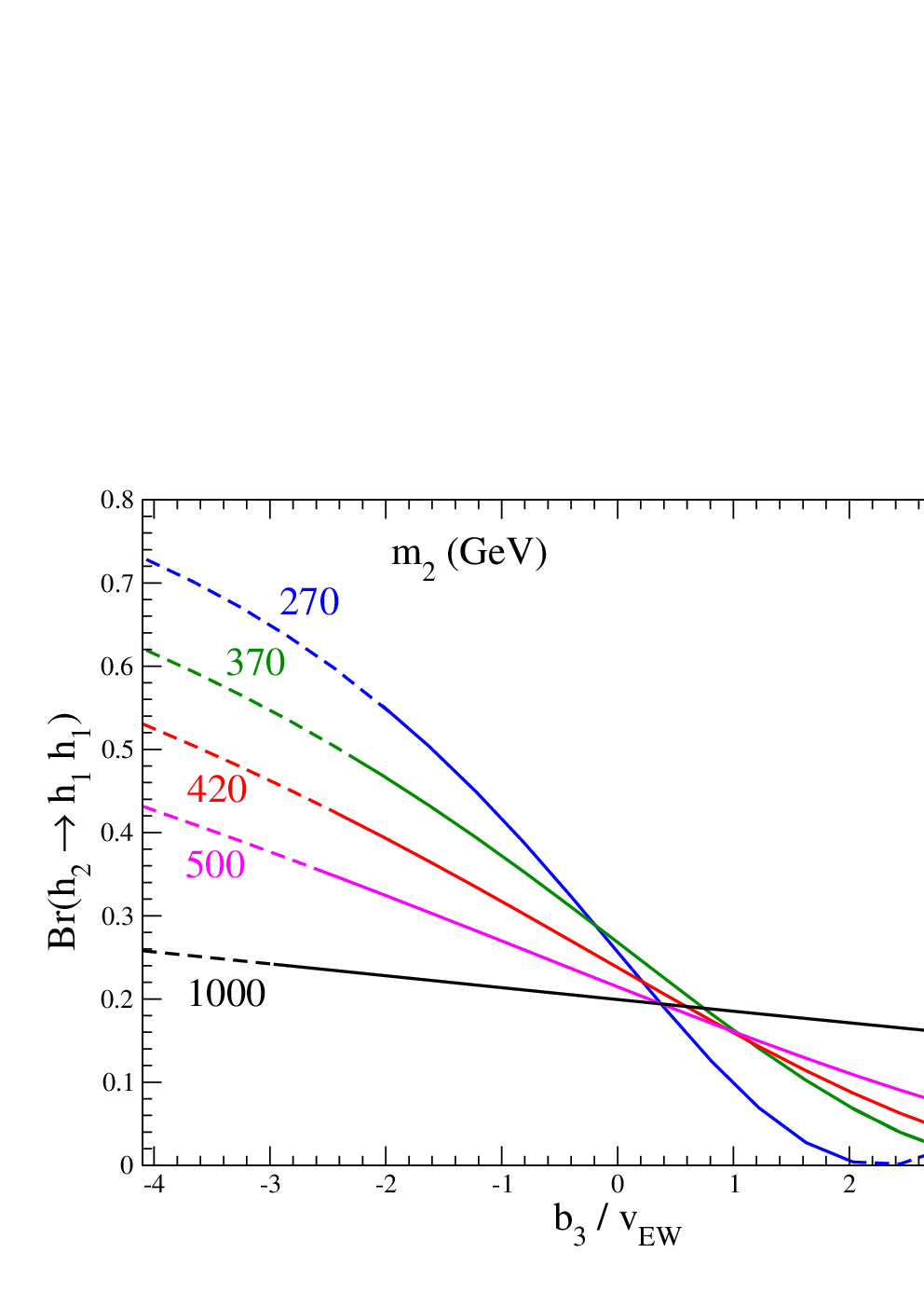
From the mass matrix in Eq. II.1, we know that varying $b_{3}$ does not change $m_{1}$, $m_{2}$ and the mixing angle $\theta$. In contrast, one can observe that $\lambda_{211}$ in Eq. 44 is a function of $b_{3}$. In Fig. 4, we show the dependence on $b_{3}$ of the branching ratio of the heavier Higgs, $h_{2}$, into the SM-like Higgs, $h_{1}$. For $b_{3}$ small, the branching ratio has little dependence on $m_{2}$, while for large $b_{3}$, the branching ratio can be large and depends significantly on $b_{3}$. The dotted curves represent regions where the parameters do not correspond to a global electroweak minimum. We see then that for a given mass this constraint corresponds to an upper limit on the branching ratio ${\rm Br}(h_{2}\rightarrow h_{1}h_{1})$.

To understand the features of Fig. 4, use the solutions in Eq. 19 to rewrite

From this we see that $b_{3}\sin(2\theta)$ and $m_{2}$ make opposite sign contributions to $\lambda_{211}$. Hence, for $b_{3}\sin(2\theta)<0$, they constructively contribute to $\lambda_{211}$. The major feature of this region in Fig. 4 is then understood by noting that the partial widths of $h_{2}$ into $h_{1}$, $W$s, and $Z$s scale like

Hence, as the mass of $h_{2}$ increases the partial widths into $W$s and $Z$s grow much more quickly than the partial width into $h_{1}h_{1}$. The branching ratio ${\rm Br}(h_{2}\rightarrow h_{1}h_{1})$ therefore decreases with mass.

The region for $b_{3}\sin(2\theta)>0$ is slightly more involved. Using Eq. 33, the triple coupling $\lambda_{211}$ goes to zero when

We see that for smaller $m_{2}$ the zero corresponds to smaller $b_{3}\sin(2\theta)$. As $b_{3}\sin(2\theta)$ goes from negative to positive, the smaller $m_{2}$ values turn over and approach zero more quickly than the larger $m_{2}$. This is the behaviour we see in Fig. 4. Note that for our representative parameters, we have $\theta>0$, so the sign of $b_{3}\sin(2\theta)$ is the same as $b_{3}$.

In Fig. 5, we plot the dependence of the ratio of the di-Higgs production cross section in the singlet model to that in the SM. In this type of model, the double Higgs production cross section can reach up to $\mathcal{O}(10)$ times that of the SM with $58\%\gtrsim{\rm Br}(h_{2}\to h_{1}h_{1})\gtrsim 28$%. Interestingly, the enhancement does not grow as $\sqrt{S}$ is increased from $14~TeV$ to $100~TeV$, although of course the total rate is increased. Both the SM and singlet rates are dominated by gluon fusion production; hence, both rates are similarly increased between $14$ and $100$ TeV.

The di-Higgs enhancement depends on the production cross section of $h_{2}$ and the branching ratio of $h_{2}\rightarrow h_{1}h_{1}$. Since the production cross section of lower mass states is generically larger than that of high mass states, $m_{2}=270$ GeV has the largest enhancement for $b_{3}<0$. For $b_{3}>0$, it is possible for the branching ratio of $h_{2}\rightarrow h_{1}h_{1}$ to go to zero. The behaviour of the enhancement in this region closely follows the discussion of Fig. 4. For $\sqrt{S}=100~TeV$ and $b_{3}<0$ (Fig. 5(b)), the cross section for $m_{2}=270~GeV$ drops below that of $m_{2}=370~GeV$. As to be discussed later, this is due to specific properties of di-Higgs production.

In Fig. 6 we show the the enhanced di-Higgs ratio as a function of the $h_{2}\rightarrow h_{1}h_{1}$ branching ratio. If the narrow width approximation holds and the production cross section $h_{2}$ is sufficiently larger than the SM di-Higgs rate, we have

Hence, we would expect this dependence to be a straight line, as seen for $m_{2}=270$ and $420$ GeV. However, we see that this is not the case for $m_{2}=1000$ GeV. In Fig. 7 we show the ratio of the total width of $h_{2}$ and $m_{2}$ as a function of the branching ratio of $h_{2}\rightarrow h_{1}h_{1}$. As can be seen for $m_{2}=1000$ GeV, the width is always large and the narrow width approximation is poor. This explains why the $m_{2}=1000$ GeV line in Fig. 6 is not straight. Also, as the branching ratio of $h_{2}\rightarrow h_{1}h_{1}$ increases, the total width become larger. This is due to the partial width $h_{2}\rightarrow h_{1}h_{1}$ becoming large, since the partial widths into $W$ and $Z$ boson is fixed by the mass $m_{2}$ and mixing angle $\theta$.

In Fig. 6, it is interesting to note that the enhancement for $m_{2}=420~GeV$ is larger than that for $270~GeV$ at $\sqrt{S}=100~TeV$. This can be understood from the parton luminosity plot of Fig. 8(a), where we show the gluon-gluon parton luminosity (normalized to that at $2m_{t}$). The $\sqrt{S}=14~TeV$ luminosity falls much more quickly as a function of invariant mass than does the corresponding luminosity at $\sqrt{S}=100~TeV$. We compare this with the resonant production of $gg\rightarrow h_{2}$ in Fig. 8(b) and observe that at $\sqrt{S}=100~TeV$ the resonant enhancement at the $t{\overline{t}}$ threshold is more important than at $\sqrt{S}=14~TeV$. Finally, we show the dependence on $m_{2}$ of the full cross section for $gg\rightarrow h_{1}h_{1}$ in Fig. 9. The resonant structure near $2m_{t}$ is clearly visible.

It may be necessary in certain models to impose a $Z_{2}$ symmetry on the potential under which $S$ is odd and $H$ is even. This may be motivated from a dark matter perspective, where $S$ is a dark matter particle, or the point of view of a complex hidden sector. The potential for this case can be obtained in the limit $a_{1},b_{1},b_{3}\rightarrow 0$. If the $Z_{2}$ remains unbroken, there is no resonance enhancement in di-Higgs production, since the $S\rightarrow hh$ decay breaks the $Z_{2}$ symmetry and there is no mixing between $S$ and $h$. We ignore this case. However, the $Z_{2}$ symmetry may be broken by a vev of $S$. Unlike the case outlined above, the vev of $S$ is then physically meaningful and we cannot set $\langle{S}\rangle=x=0$ arbitrarily. The $Z_{2}$ symmetric potential is,

We shift the fields in the usual manner to find the $h_{2}h_{1}h_{1}$ coupling in the $Z_{2}$ symmetric limit[10],

In the limit $x=0$ and $a_{1},b_{1}$, and $b_{3}=0$, Eq. 38 is in agreement with Eq. 44. We impose the conditions of positivity of the potential, $\lambda>0,b_{4}>0$ and $4\lambda b_{4}-a_{2}^{2}>0$ (Eq. 24) and require the couplings to be perturbative, $a_{2},b_{4},\lambda<4\pi$.

The physical parameters are taken as,

Using Eqs. 38 and 22, the branching ratio for $h_{2}\rightarrow h_{1}h_{1}$ can be found and is shown in Fig. 10. Comparing with Fig. 6, it is apparent that the branching ratios are similar in the models with and without the $Z_{2}$ symmetry for large values of $x/v_{EW}$, where the branching ratio asymptotes to around $BR(h_{2}\rightarrow h_{1}h_{1})\sim 0.3$. The branching ratio $h_{2}\rightarrow h_{1}h_{1}$ appears to have little discriminating power between the $Z_{2}$ symmetric and non-symmetric potentials.

From the direct measurements of the Higgs coupling strengths, ATLAS [33] places a constraint on the mixing angle, $\theta$, of the singlet model, where $\cos^{2}\theta\leq 0.88$ has been excluded at 95% CL. This limit assumes that there is no branching ratio to invisible particles. Here we take the upper limit of $\sin^{2}\theta\leq 0.12$ as a representative point. Direct searches for the heavy Higgs ($h_{2}$) decaying into $W^{+}W^{-}$ and $ZZ$ from ATLAS and CMS [34, 35] can also give bounds on $\sin^{2}\theta$ with $\sin^{2}\theta\lesssim 0.2$ for $m_{2}\sim 200-400$ GeV and $\sin^{2}\theta\lesssim 0.4$ for $m_{2}\sim 600$ GeV. However, these constraints are not as strong as the ATLAS limit from the Higgs coupling strengths.

The existence of a Higgs singlet which mixes with the SM Higgs boson is also restricted by electroweak precision observables. A fit to the oblique parameters, $S$ and $T$ (fixing $U$ to be $0$), is shown in Fig. 11 [36, 20]. We see that limits from the oblique parameters are not competitive with the ATLAS limit from the Higgs coupling strengths.

ATLAS and CMS have obtained upper bounds on the cross section for the resonant production of SM Higgs bosons pairs through the process $pp\rightarrow h_{2}^{*}\rightarrow h_{1}h_{1}$ in the $\gamma\gamma b{\bar{b}}$ [37, 38] and $b{\bar{b}}b{\bar{b}}$ [39] channels at a center-of-mass energy of $\sqrt{S}=8~TeV$ with an integrated luminosity of  $20~fb^{-1}$ as summarized in Fig. 12. In the low mass region the $\gamma\gamma b{\bar{b}}$ channel gives a stronger bound as opposed to a weaker bound obtained in the $b{\bar{b}}b{\bar{b}}$ channel due to the large QCD background. However, the limit from the $b{\bar{b}}b{\bar{b}}$ channel becomes more constraining above $m_{2}\sim 400$ GeV.

We compare the experimental upper limits on the production cross sections for resonant di-Higgs production with $m_{2}$ between $270~GeV$ and $1~TeV$, normalized to the leading order cross section predicted by the SM, with the range of allowed cross sections consistent with the requirement that the parameters correspond to a global electroweak minimum. (The allowed region is between the curves). Two sets of parameter points $(b_{4},a_{2})=(3,0)$ and $(b_{4},a_{2})=(1,-1)$ are considered. The former has a larger value of $b_{4}$ and hence the bound is less stringent as illustrated in Fig. 2(b). The lower limit of the allowed region on $m_{2}$, which starts at $m_{2}\sim 370$ GeV, for $(b_{4},a_{2})=(1,-1)$ can be explained by Eq. 26 as due to the vacuum stability constraint. Plugging in $\lambda$ defined in Eq. 19, one can obtain the lower limit for $m_{2}^{2}$ for a given $b_{4}$ and negative $a_{2}$,

Throughout the $m_{2}<1~TeV$ mass range, the constraints derived from the global electroweak minimum requirement are always stronger than those currently available from the LHC experiments at $\sqrt{S}=8$ TeV. We make naive projections for the expected constraints at the LHC at $\sqrt{S}=14$ TeV with an integrated luminosity of $300~fb^{-1}$ by rescaling the expected $95\%$ CL upper limits at $\sqrt{S}=8$ TeV with an integrated luminosity of $20~fb^{-1}$, using the ratios of gluon-gluon luminosities (evaluated at the scale $2m_{1}$) given in Ref. [40]. As shown in Fig. 13, the projected bounds from the CMS $\gamma\gamma b{\bar{b}}$ channel can rule out the entire parameter space where the electroweak minimum is a global minimum for $(b_{4},a_{2})=(1,-1)$ and can exclude much of the allowed region for $(b_{4},a_{2})=(3,0)$. Moreover, the projected limits from the CMS $b{\bar{b}}b{\bar{b}}$ channel can potentially exclude the entire parameter space allowed by the electroweak minimum requirement for $(b_{4},a_{2})=(1,-1)$ and rule out two thirds of the allowed region in the high mass range for $(b_{4},a_{2})=(3,0)$.

The coefficients of the potential cannot be too large or perturbative unitarity will be violated in the $h_{i}h_{j}$ scattering processes [41]. The simplest limit comes from the high energy scattering of $h_{2}h_{2}\rightarrow h_{2}h_{2}$, where the $J=0$ partial wave is,

Requiring $\mid a_{0}\mid<{1\over 2}$ yields $\mid b_{4}\mid\leq 4.2$. Limits from a coupled channel analysis of $h_{i}h_{j}$ scattering show that for small $\sin\theta$, multi-TeV scale masses are allowed for $m_{2}$ [10].

Similarly, we can consider the $h_{1}h_{1}\rightarrow h_{1}h_{1}$ scattering to find the $J=0$ partial wave.

Then using Eq. 19 and $\mid a_{0}\mid<{1\over 2}$, an upper limit on $m_{2}$ can be found:

For $\cos^{2}\theta=0.88$ and $m_{1}=126$ GeV, this limit is $m_{2}\lesssim 2$ TeV.

References

- [1] T. Plehn, M. Spira, and P. Zerwas, Nucl.Phys. B479, 46 (1996), hep-ph/9603205.
- [2] U. Baur, T. Plehn, and D. L. Rainwater, Phys.Rev. D67, 033003 (2003), hep-ph/0211224.
- [3] J. Baglio et al., JHEP 1304, 151 (2013), 1212.5581.
- [4] LHC Higgs Cross Section Working Group, S. Dittmaier et al., (2011), 1101.0593.
- [5] R. Frederix et al., Phys.Lett. B732, 142 (2014), 1401.7340.
- [6] M. J. Dolan, C. Englert, and M. Spannowsky, JHEP 1210, 112 (2012), 1206.5001.
- [7] S. Dawson, S. Dittmaier, and M. Spira, Phys.Rev. D58, 115012 (1998), hep-ph/9805244.
- [8] D. de Florian and J. Mazzitelli, PoS LL2014, 029 (2014), 1405.4704.
- [9] J. Grigo, K. Melnikov, and M. Steinhauser, Nucl.Phys. B888, 17 (2014), 1408.2422.
- [10] G. M. Pruna and T. Robens, Phys.Rev. D88, 115012 (2013), 1303.1150.
- [11] V. Barger, P. Langacker, M. McCaskey, M. J. Ramsey-Musolf, and G. Shaughnessy, Phys.Rev. D77, 035005 (2008), 0706.4311.
- [12] D. O’Connell, M. J. Ramsey-Musolf, and M. B. Wise, Phys.Rev. D75, 037701 (2007), hep-ph/0611014.
- [13] S. Profumo, M. J. Ramsey-Musolf, C. L. Wainwright, and P. Winslow, (2014), 1407.5342.
- [14] M. Bowen, Y. Cui, and J. D. Wells, JHEP 0703, 036 (2007), hep-ph/0701035.
- [15] V. Barger, L. L. Everett, C. Jackson, A. Peterson, and G. Shaughnessy, (2014), 1408.0003.
- [16] M. J. Dolan, C. Englert, and M. Spannowsky, Phys.Rev. D87, 055002 (2013), 1210.8166.
- [17] R. Schabinger and J. D. Wells, Phys.Rev. D72, 093007 (2005), hep-ph/0509209.
- [18] C. Englert, T. Plehn, D. Zerwas, and P. M. Zerwas, Phys.Lett. B703, 298 (2011), 1106.3097.
- [19] C. Englert, T. Plehn, M. Rauch, D. Zerwas, and P. M. Zerwas, Phys.Lett. B707, 512 (2012), 1112.3007.
- [20] S. Profumo, M. J. Ramsey-Musolf, and G. Shaughnessy, JHEP 0708, 010 (2007), 0705.2425.
- [21] J. R. Espinosa, T. Konstandin, and F. Riva, Nucl.Phys. B854, 592 (2012), 1107.5441.
- [22] D. Curtin, P. Meade, and C.-T. Yu, (2014), 1409.0005.
- [23] M. Gillioz, R. Grober, C. Grojean, M. Muhlleitner, and E. Salvioni, JHEP 1210, 004 (2012), 1206.7120.
- [24] S. Dawson, E. Furlan, and I. Lewis, Phys.Rev. D87, 014007 (2013), 1210.6663.
- [25] C.-Y. Chen, S. Dawson, and I. Lewis, Phys.Rev. D90, 035016 (2014), 1406.3349.
- [26] J. Baglio, O. Eberhardt, U. Nierste, and M. Wiebusch, Phys.Rev. D90, 015008 (2014), 1403.1264.
- [27] B. Hespel, D. Lopez-Val, and E. Vryonidou, JHEP 1409, 124 (2014), 1407.0281.
- [28] B. Bhattacherjee and A. Choudhury, (2014), 1407.6866.
- [29] A. Arhrib, R. Benbrik, C.-H. Chen, R. Guedes, and R. Santos, JHEP 0908, 035 (2009), 0906.0387.
- [30] N. Craig, J. Galloway, and S. Thomas, (2013), 1305.2424.
- [31] J. M. No and M. Ramsey-Musolf, Phys.Rev. D89, 095031 (2014), 1310.6035.
- [32] J. F. Gunion, H. E. Haber, G. L. Kane, and S. Dawson, Front.Phys. 80, 1 (2000).
- [33] A. Collaboration, Constraints on New Phenomena via Higgs Boson Coupling Measurements with the ATLAS Detector.
- [34] CERN Report No. ATLAS-CONF-2013-067, 2013 (unpublished).
- [35] CMS Collaboration, S. Chatrchyan et al., Eur.Phys.J. C73, 2469 (2013), 1304.0213.
- [36] S. Dawson and W. Yan, Phys.Rev. D79, 095002 (2009), 0904.2005.
- [37] ATLAS Collaboration, G. Aad et al., (2014), 1406.5053.
- [38] CMS Collaboration, CERN Report No. CMS-PAS-HIG-13-032, 2014 (unpublished).
- [39] CMS Collaboration, CERN Report No. CMS-PAS-HIG-14-013, 2014 (unpublished).
- [40] C. Quigg, (2011), 1101.3201.
- [41] B. W. Lee, C. Quigg, and H. Thacker, Phys.Rev. D16, 1519 (1977).