Conditional Preference Orders and their Numerical Representations

In decision theory, the normative framework of preference ordering classically requires the completeness axiom. Yet, there are good reasons to question completeness as famously pointed out by Aumann [2]:

Of all the axioms of utility theory, the completeness axiom is perhaps the most questionable. […] For example, certain decisions that an individual is asked to make might involve highly hypothetical situations, which he will never face in real life. He might feel that he cannot reach an “honest” decision in such cases. Other decision problems might be extremely complex, too complex for intuitive “insight”, and our individual might prefer to make no decision at all in these problems. Is it “rational” to force decision in such cases?

Aumann’s remark, supported by empirical evidence, triggered intensive research in terms of interpretation, axiomatization and representation of general incomplete preferences, see [37, 34, 3, 15, 16, 18, 20] and the references therein. These authors consider incompleteness either as a result of status quo, see Bewley [3], or procedural decision making, see Dubra and Ok [15], and the numerical representations are in terms of multi-utilities. However, Aumann’s quote and a correspondence with Savage [38], where he exposes the idea of state-dependent preferences, suggest that the lack of information underlying a decision making is a natural source of incompleteness. For instance, consider the simple situation where a person has to decide between visiting a museum or going for a walk on Sunday in one month from now. She cannot express an unequivocal preference between these two prospective situations since it depends on the knowledge of uncertain factors like the weather, availability of an accompanying person, etc. This information-based incompleteness suggests a contingent form of completeness. For instance, conditioned on the event “sunny and warm day” she prefers a walk. In this way, a complex decision problem, provided sufficient information, leads to an “honest” decision. The present work suggests a framework formalizing this idea of a contingent decision making and its quantification.

Numerous quantification instruments in finance and economics entail a conditional dimension by mapping prospective outcomes to random variables such as for instance conditional and dynamic monetary risk measures [11, 7, 6, 1], conditional expected utilities and certainty equivalents, dynamic assessment indices [24, 4] or recursive utilities [19, 17]. However, few papers address the axiomatization of conditional preferences underlying these conditional quantitative instruments. In this direction is the work of Luce and Krantz [31] where an event-dependent preference ordering is considered and studied. Their approach is further refined and extended in Wakker [42] and Karni [27], Karni [28]. State-wise dependency is used in Kreps and Porteus [29], Kreps and Porteus [30] and Maccheroni et al. [32] to study intertemporal preferences and a dynamic version of preferences, respectively. Remarkable is the abstract approach by Skiadas [39], Skiadas [40]. He provides a set of axioms modeling conditional preferences on random variables which admit a conditional Savage representation of the form

where $\mathcal{A}$ is an algebra of events representing the information, $Q$ is a subjective probability measure and $u$ is a utility index. As in the previous works, its decision-theoretical foundation consists of a whole family of total pre-orders $\succcurlyeq^{A}$, one for each event $A\in\mathcal{A}$, and a consistent aggregation property in order to obtain the conditional representation. However, the decision maker is assumed to implicitly take into account a large number ¹¹ 1 In a five steps binary tree, $4.294.967.296$ is the cardinality of the family of total pre-orders $\succcurlyeq^{A}$. of complete pre-orders.

Our axiomatic approach differs in so far as it considers a single but possibly incomplete preference order $\succcurlyeq$ instead of a whole family of complete preference orders. Even if one cannot a priori decide whether $x\succcurlyeq y$ or $y\succcurlyeq x$ for any two prospective outcomes, or acts, there may exist a contingent information $A$ conditioned on which $x$ is preferable to $y$. In this case we formally write $x|A\succcurlyeq y|A$. The set of contingent information is modeled as an algebra of events $\mathcal{A}=(\mathcal{A},\cap,\cup,{}^{c},\emptyset,\Omega)$ of a state space $\Omega$.²² 2 Conditional set theory [14] allows the contingent information to be any complete Boolean algebra. In order to describe the conditional nature of the preference, we require that $\succcurlyeq$ interacts consistently with the information, that is,

• •

  consistency: if $x|A\succcurlyeq y|A$ and $B\subseteq A$, then $x|B\succcurlyeq y|B$;

• •

  stability: if $x|A\succcurlyeq y|A$ and $x|B\succcurlyeq y|B$, then $x|A\cup B\succcurlyeq y|A\cup B$;

• •

  local completeness: for every two acts $x$ and $y$ there exists a non-empty event $A$ such that either $x|A\succcurlyeq y|A$ or $x|A\succcurlyeq y|A$.

These assumptions bear a certain normative appeal in view of the conditional approach that we are aiming at. In the context of the previous example, consistency says that if the person prefers a walk over a visit to a museum whenever it is ‘‘sunny’’ or ‘‘warm’’, then a fortiori she prefers a walk if it is ‘‘sunny’’. Stability tells that if she prefers a walk whenever it is ‘‘sunny’’ or ‘‘rainy’’, then on any day where at least one of these conditions is met she will go for a walk. In contrast to classical preferences, we only assume a local completeness: For any two situations she is able to meet a decision provided enough -- possibly extremely precise³³ 3 Indeed, the smaller the event, the more precise in which state of the world this event may occur. The most precise event being the singleton. – information. In our example, there exists a rather unlikely, but still non-trivial, coincidence of the conditions ‘sunny’, ‘humidity between 15 and 20%’ and ‘wind between 0 and 10km/h’ under which she prefers a walk to the museum. Unlike classical completeness, the information necessary to decide between two acts $x$ and $y$ depends on the pair $(x,y)$. Note that if the set of contingent information reduces to the trivial information $\mathcal{A}=\{\emptyset,\Omega\}$, then, as expected, a conditional preference is a classical complete preference order. In particular, classical decision theory is a special case of the conditional one.

Observe that our approach, as [31, 42, 29, 39, 40], considers an exogenously given set of informations or events as the source of incomplete decision making. Whereas in [3, 15] and the related subsequent literature on incomplete preference, the incompleteness and the resulting multi-valued representations yield an endogenous information about the nature of the incompleteness. Incompleteness there is however not in terms of an algebra of events, and therefore not specifically related to a contingent decision making.

Our approach is also not a priori dynamic in the sense that a single algebra of available information is given for the contingent decision making. We do not address the question of progressive learning over time as new information reveals, resulting in an update of decisions. This incremental learning approach in decision making is investigated by Kreps and Porteus [29], and recently by Dillenberger et al. [12] as well as Piermont et al. [35].⁴⁴ 4 Though, Dillenberger et al. [12] consider a static approach resulting in dynamic utility valuations that are deterministic. In these articles, the agent learns over time and may modify her behavior according to the new information as well as her previous choice making. However, the underlying information structure is exogenously given – either by a fixed dynamic structure by means of a filtration or a random tree, or by the filtration generated by the consumption paths, or even by the filtration generated by the previous preference orders. Our approach may help in these cases by considering a sequence of conditional preference orders $\succcurlyeq_{0},\succcurlyeq_{1},\ldots,\succcurlyeq_{t},\ldots$ with respect to an increasing sequence of algebra of events $\mathcal{A}_{0}\subseteq\mathcal{A}_{1}\subseteq\cdots\subseteq\mathcal{A}_{t}\subseteq\cdots$ each of which for every point in time. We can provide an axiomatic system to describe these conditional preference orders $\succcurlyeq_{t}$ for each given time $t$, and derive a sequence of conditional numerical representations $U_{t}$. Since we only address the case of a single information structure, that is, at a fixed given time $t$, we intentionally left out the following two questions in the dynamic context. First, whether the decision making at time $t$ is influenced by the past information, that is a Markovian versus non-Markovian decision making. Second, the impact at time $t$ of past and eventually future decisions. In other terms, the interdependence structure over time of these preferences and the consequences for the dynamic utility representation⁵⁵ 5 For instance, time consistency, Bellman principle, weaker time consistency, etc. in terms of time consistency.⁶⁶ 6 A topic of intensive study in mathematical finance, see [7, 6, 1, 8, 4] among others.

Although being intuitive, it is mathematically not obvious what is meant by a contingent prospective act $x|A$. The formalization of which corresponds to the notion of a conditional set, introduced recently by Drapeau et al. [14]. An heuristic introduction to conditional sets is given in Section 2. For an exhaustive mathematical presentation we refer to [14]. The formalization and properties of conditional preferences are given in Section 3. In Section 4, we address the notion of conditional numerical representation and prove a conditional version of Debreu’s existence result of continuous numerical representations. While the proof technique differs, the classical statements in decision theory translate into the conditional framework. For instance, a conditional version of the classical representation of von Neumann and Morgenstern [41] is presented in Section 5. The representation of Debreu requires topological assumptions that often are not met in practice. In Section 6, we provide conditional results that allow to extend Debreu and Rader’s theorem in a more general framework, and present automatic continuity results which allow to bypass topological assumptions. We illustrate each of these cases by examples. These results in their classical form rely on the Gap Lemma of Debreu [9], Debreu [10] the conditional adaptation of which does not involve any measurable selection arguments but derives from a conditional version of the axiom of choice. Section 7 is dedicated to the formulation and the proof of this conditional Gap Lemma. In Appendix A, we gather some technical results and most of the proofs.

As mentioned in the introduction, we model the contingent information, conditioned on which a decision maker ranks prospective outcomes, by an algebra of events $\mathcal{A}$. For technical reasons, we assume that it is a $\sigma$-algebra with a probability measure defined on it. The inclusion of two events is then to be understood in the almost sure sense.⁷⁷ 7 In the theory of conditional sets, any complete algebra can be considered as a source of information and what follows also holds in this slightly more general framework. Though, from an economical point of view, most standard frameworks consider finite algebras of events or $\sigma$-algebras with a probability measure on it that describe the events of null measure, that is, those events that are considered as never occurring. A $\sigma$-algebra on which sets are identified if they coincide almost surely is complete, see [25, 14]. If one does not want to consider probability spaces, the Borel sets of a Polish space factorised by the sets of category one is a complete Boolean algebra. A set $X$ – that in the present context describes acts – is a conditional set of $\mathcal{A}$ if it allows for conditioning actions $A:X\to X|A$ for each event $A\in\mathcal{A}$ which satisfy a consistency and an aggregation property:

• Consistency: For any two acts $x,y\in X$ and events $A\subseteq B$, if the acts $x$ and $y$ coincide conditioned on $B$, that is, $x|B=y|B$, then they also coincide conditioned on $A$, that is, $x|A=y|A$.

• Stability: For any two acts $x,y\in X$ and event $A\in\mathcal{A}$, there exists an act $z\in X$ such that $z$ coincides with $x$ conditioned on $A$ and with $y$ otherwise. We denote this element $z=x|A+y|A^{c}$.⁸⁸ 8 Since we assume that $\mathcal{A}$ can be made complete, the concatenation property is required for any partition of events $(A_{i})\subseteq\mathcal{A}$ and family of acts $(x_{i})\subseteq X$, and we denote $x=\sum x_{i}|A_{i}$ the unique element such that $x$ coincides with $x_{i}$ conditioned on $A_{i}$.

Intuitively, the action $x\mapsto x|A$ tells how acts are conditioned on the information $A$ and $X|A$ represents the acts in $x$ conditioned to $A$.

The relation between conditional sets is described by the conditional inclusion which is characterized by two dimensions, a classical inclusion and a conditioning:

• •

  On the one hand, every non-empty set $Y\subseteq X$ which is stable, that is, $x|A+y|A^{c}\in Y$ for every $x,y\in Y$ and $A\in\mathcal{A}$, is a conditional subset of $X$.

• •

  On the other hand, $X|A$ is a conditional set but on the relative algebra $\mathcal{A}_{A}:=\{B\cap A\colon B\in\mathcal{A}\}$ and a subset of $X$ conditioned on $A$.

Combining the two dimensions, a conditional set $Y$ is said to be conditionally included in $X$, denoted $Y\sqsubseteq X$, if $Y=Z|A$ for some stable $Z\subseteq X$ and a condition $A\in\mathcal{A}$. In that case, we say that $Y$ is a conditional set “living” on $A$ and if we want to emphasize the condition on which this conditional set lives, we denote it $Y|A$. The conditional inclusion is illustrated in Figure 1(a). If $A=\emptyset$, then $X|\emptyset$ lives nowhere and in particular is conditionally contained in any conditional set, and thus is conditionally the emptyset. The conditional powerset

consists of the collection of all conditional subsets of $X$.

The conditional intersection of two conditional sets $Y,Z$ is the intersection on the largest condition $A^{\ast}$ on which $Y$ and $Z$ have a non-empty classical intersection as illustrated in Figure 1(b).

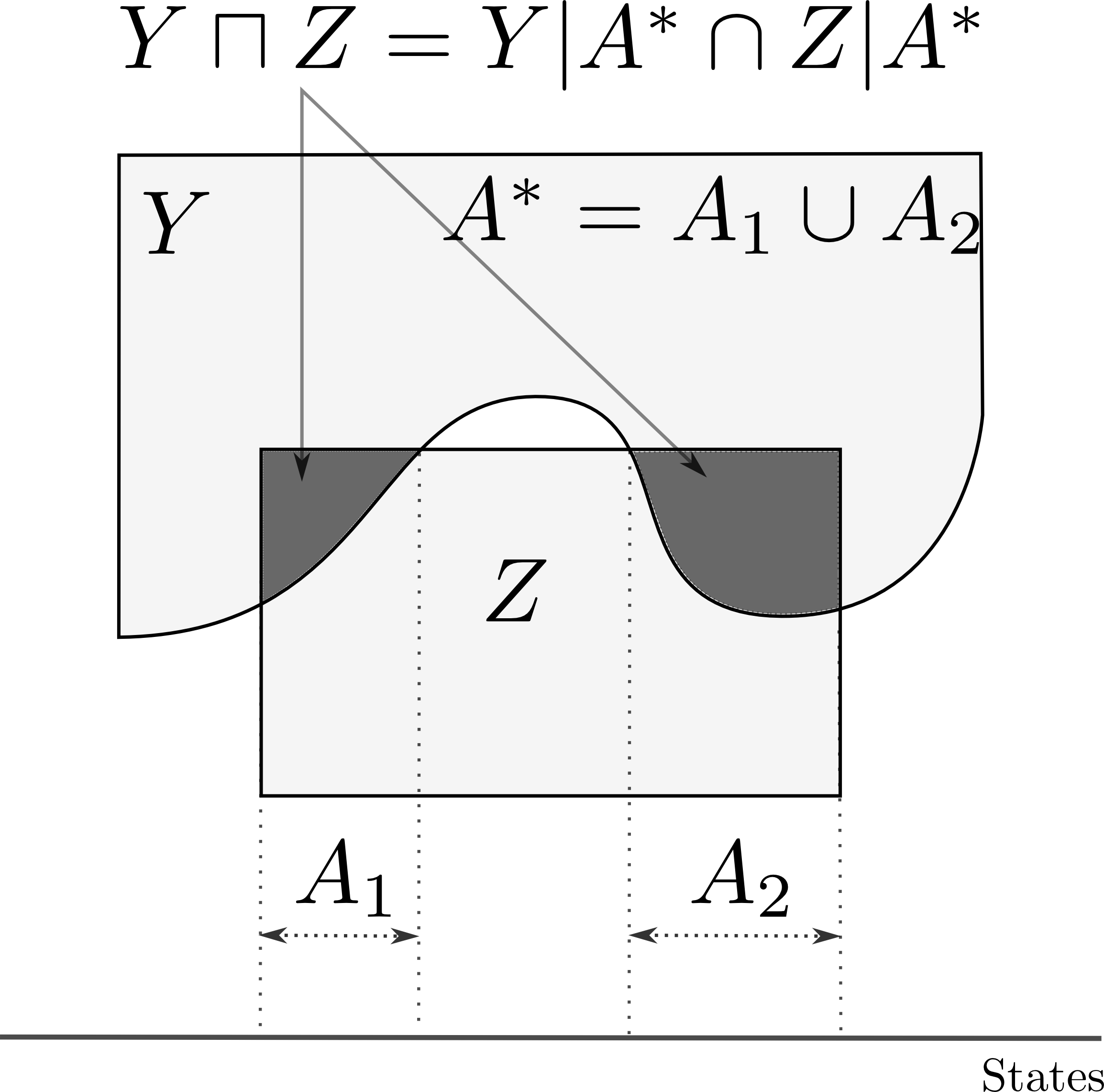
The conditional union of two conditional subsets $Y,Z$ is the collection of all elements which can be concatenated such that each piece of the concatenation conditionally falls either in $Y$ or in $Z$. The conditional union is defined by

and illustrated in Figure 2(a). Finally, the conditional complement $Y^{\sqsubset}$ of a conditional subset $Y$ is the collection of all those elements $y$ which nowhere fall into $Y$, as illustrated in Figure 2(b).

A main result in [14] is that the conditional powerset together with these operations forms a complete Boolean algebra

Following the classical constructions, the conditional powerset allows to define conditional relations, and functions, and topologies, and other conditional structures, see [14].

For the remainder of the paper $X$ denotes a conditional set. A conditional binary relation $\succcurlyeq$ is a conditional subset $G\sqsubseteq X\times X$ living on $\Omega$ and we write $x\succcurlyeq y$ if and only if $(x,y)\in G$. In particular, a conditional binary relation is at first a classical binary relation. However, due to the fact that the graph $G$ is a conditional set and writing $x|A\succcurlyeq y|A$ for $(x|A,y|A)\in G|A$, the following additional properties hold

• •

  consistency: if $x|A\succcurlyeq y|A$ and $B\subseteq A$, then $x|B\succcurlyeq y|B$;

• •

  stability: if $x|A\succcurlyeq y|A$ and $x|B\succcurlyeq y|B$, then $x|A\cup B\succcurlyeq y|A\cup B$;

corresponding to two of the normative properties mentioned in the introduction. Given a conditional binary relation, $\sim$ denotes the symmetric part of the binary relation and we use the notation

In other words, $x\succ y$ means that $x$ is strictly preferred to $y$ on any non-empty condition. Both $\sim$ and $\succ$ are conditional binary relations.

Although a conditional preference is not total, the following lemma shows that local completeness allows to derive for every two elements a partition on which a comparison can be achieved.

Next we address the quantification of such a conditional ranking. First, we need the notion of a conditional function. A conditional function $f:X\to Y$ between two conditional sets is a classical function with the additional property of stability:

For the quantification, we secondly need a conditional analogue of the real line which allows to represent the conditional preferences. The conditional real numbers, denoted by $\mathbf{R}$, are obtained from the conditional rational numbers by adapting Cantor’s construction, that is, identifying conditional Cauchy sequences in $\mathbf{Q}$. As in the standard theory, the conditional real numbers can be characterized as a conditional field where every bounded subset has an infimum and a supremum and which is topologically conditionally separable. In particular, $\mathbf{Q}$ is conditionally dense in $\mathbf{R}$.

Note that every conditional function $U:X\to\mathbf{R}$ defines a conditional preference order by means of (1). Furthermore, if $U:X\to\mathbf{R}$ is a conditional numerical representation, then $\varphi\circ U$ is a conditional numerical representation for every conditionally strictly increasing function $\varphi:\mathbf{R}\to\mathbf{R}$.

Given a conditional preference order, we address the necessary and sufficient conditions under which a conditional numerical representation exists. The first result is a conditional version of Debreu’s statement in [9] and necessitates the notion of conditionally order dense. A conditional subset $Z\sqsubseteq X$ is conditionally order dense if for every $x,y\in X$ with $x\succ y$, there exists $z\in Z$ such that $x\succcurlyeq z\succcurlyeq y$. The case of interest is when $Z$ is conditionally countable, that is, there exists a conditional injection $\varphi:Z\to\mathbf{Q}$. Equivalently, $Z$ is conditionally countable if it is a conditional sequence $Z=(z_{n})_{n\in\mathbf{N}}$ where $\mathbf{N}$ is the conditional natural numbers. There exists a difference between a conditional sequence and a standard sequence: Analogous to the classical case, a conditional sequence $(z_{n})$ in $Z$ is a conditional function $f:\mathbf{N}\to Z$, $n\mapsto f(n)=z_{n}$. However stability yields $z_{n}|A+z_{m}|A^{c}=f(n)|A+f(m)|A^{c}=f(n|A+m|A^{c})=z_{n|A+m|A^{c}}$. In other words, the sequence step $n$ conditioned on $A$ and the sequence step $m$ conditioned on $A^{c}$ result into the sequence step $n|A+m|A^{c}$.

The existence of a conditionally countable order dense subset is rather of technical nature. In the classical case, Debreu [9], Debreu [10] and then Rader [36] showed that under some topological assumptions a numerical representation exists. And even more, by means of Debreu’s Gap Lemma, the existence of an upper semi-continuous or continuous representation is guaranteed. The conditional counterparts of these results also hold, based on a conditional adaptation of Debreu’s Gap Lemma in Section 7.

A classical class of preferences are the affine ones and the resulting affine numerical representation due to von Neumann and Morgenstern [41]. This representation can be carried over to the conditional case as follows. Let $X$ be a conditionally convex subset living on $1$ of some conditional vector space. We say that a conditional preference order on $X$ satisfies the

• •

  conditional independence axiom: if $x\succ y$ then $\alpha x+(1-\alpha)z\succ\alpha y+(1-\alpha)z$ for every $z\in X$ and each $\alpha\in]0,1]$;

• •

  conditional Archimedean axiom: if $x\succ y\succ z$ then $\alpha x+(1-\alpha)z\succ y\succ\beta x+(1-\beta)z$ for some $\alpha,\beta\in]0,1[$.

A conditional real-valued numerical representation $U$ of $\succcurlyeq$ is conditionally affine, if

for every $x,y\in X$ and each $\alpha\in[0,1]$.

The result of Neumann and Morgenstern goes a step forward by providing a utility index against which lotteries are ranked according to expectation. In our context, following Example 2.4, conditional lotteries on the real line is the conditional set

where $P$ denotes a set of deterministic lotteries on the real line.¹⁸¹⁸ 18 These are related to conditional distribution on the conditional real line $\mathbf{R}$, see Jamneshan et al. [26] for the construction and definition of such conditional probability distributions. We endow this conditional set with the conditional weak^∗ topology generated by the conditional set of bounded functions

where $C_{b}$ is the set of continuous functions from the real line into the real line. In other words, a function $u\in C_{b}(\mathcal{A})$ is a state-dependent continuous function $u(\omega,x)$, that is, a state-dependent utility index. The conditional scalar product is given by the random variable

which is an element of $\mathbf{R}=L^{0}(\mathcal{A})$. In this framework, the classical representation theorem of von Neumann and Morgenstern carries over as follows.

As in the classical case, the assumptions of Theorem 4.9 are empirically as well as mathematically problematic for the following reasons

• •

  Many of the topologies of interest for practical representations are not second countable, not even metrizable;

• •

  Requiring upper semi-continuity is an empirical issue in particular for non-metrizable topologies since it is not practically falsifiable.

An answer to the first point is the following proposition that relies on a conditional version of Banach-Alaoglu based on the notion of conditional compactness introduced in [14].

As for the second question, we show that automatic continuity results taking advantage of monotonicity also extends to the continuous case and yields the following result.

Let us illustrate this automatic continuity result in the framework presented in [4]. By $x_{t},x_{t+1},\ldots,x_{T}$ we denote a future cumulative cash-flow stream starting from a given future time $t$. We are interested in the study of an investor’s assessment $\succcurlyeq$ of these future cash-flows but conditioned on the available information at this time $\mathcal{A}:=\mathcal{A}_{t}$. The information at time $s$ is denoted by $\mathcal{A}_{s}$ and it holds $\mathcal{A}_{s}\subseteq\mathcal{A}_{s+1}$ for every $s\geq t$. The cash-flow $x_{s}$ is adapted to $\mathcal{A}_{s}$ and is square integrable, that is $E[\left|x_{s}\right|^{2}|\mathcal{A}_{t}]<\infty$. We denote by

which is a conditionally reflexive Hilbert space, see [14, 22]. We denote by

• •

  $\Delta$ the set of probability measures $Q$ absolutely continuous with respect to the reference measure;

• •

  $\mathcal{D}$ the set of discounting factors, that is those processes $D=(D_{t},\ldots,D_{T})$ where $1=D_{t}\geqslant D_{t+1}\geqslant\ldots\geqslant D_{T}\geqslant 0$ where $D_{s}$ is $\mathcal{A}_{s-1}$ adapted.

It follows that

References

- [1] B. Acciaio, H. Föllmer, and I. Penner. Risk assessment for uncertain cash flows: Model ambiguity, discounting ambiguity, and the role of bubbles. Forthcoming in Finance and Stochastics, 2011.
- [2] R. J. Aumann. Utility theory without the completeness axiom. Econometrica, 30(3):445–462, 1962.
- [3] T. F. Bewley. Knightian decision theory. Part I. Decisions in Economics and Finance, 2001.
- [4] T. R. Bielecki, I. Cialenco, S. Drapeau, and M. Karliczek. Dynamic assessment indices. Stochastics. An International Journal of Probability and Stochastic Processes (forthcoming), 2014.
- [5] S. Cerreia-Vioglio, F. Maccheroni, M. Marinacci, and L. Montrucchio. Uncertainty averse preferences. Journal of Economic Theory, 146(4):1275–1330, 2011.
- [6] P. Cheridito and M. Kupper. Recursivity of indifference prices and translation-invariant preferences. Mathematics and Financial Economics, 2:173–188, 2009.
- [7] P. Cheridito, F. Delbaen, and M. Kupper. Dynamic monetary risk measures for bounded discrete-time processes. Electronic Journal of Probability, 11(3):57–106, 2006.
- [8] I. Cialenco, T. R. Bielecki, and Z. Zhang. Dynamic coherent acceptability indices and their applications to finance. To appear in Mathematical Finance, 2010.
- [9] G. Debreu. Representation of a preference ordering by a numerical function. In C. C. Thrall, R.M. and R. Davis, editors, Decision Process, pages 159–165. John Wiley, New York, 1954.
- [10] G. Debreu. Continuity properties of Paretian utility. International Economic Review, 5(3):285–293, 1964.
- [11] K. Detlefsen and G. Scandolo. Conditional and dynamic convex risk measures. Finance and Stochastics, 9:539–561, 2005.
- [12] D. Dillenberger, J. S. Lleras, P. Sadowski, and N. Takeoka. A theory of subjective learning. Journal of Economic Theory, 153:287–312, 2014. ISSN 0022-0531.
- [13] S. Drapeau and M. Kupper. Risk preferences and their robust representation. Mathematics of Operations Research, 28(1):28–62, 2013.
- [14] S. Drapeau, A. Jamneshan, M. Karliczek, and M. Kupper. The algebra of conditional sets and the concepts of conditional topology and compactness. Journal of Mathematical Analysis and Applications (forthcoming), 2013.
- [15] J. Dubra and E. A. Ok. A model of procedural decision making in the presence of risk. International Economic Review, 43(4):1053–1080, 2002.
- [16] J. Dubra, F. Maccheroni, and E. A. Ok. Expected utility theory without the completeness axiom. Journal of Economic Theory, 115(1):118–133, 2004.
- [17] D. Duffie and L. G. Epstein. Stochastic differential utility. Econometrica, 60(2):353–94, 1992.
- [18] K. Eliaz and E. A. Ok. Indifference or indecisiveness? Choice-theoretic foundations of incomplete preferences. Games and Economic Behavior, 56(1):61 – 86, 2006.
- [19] L. G. Epstein and S. E. Zin. Substitution, risk aversion, and the temporal behavior of consumption and asset returns: A theoretical framework. Econometrica, 57(4):937–69, 1989.
- [20] O. Evren and E. A. Ok. On the multi-utility representation of preference relations. Journal of Mathematical Economics, 47(4-5):554–563, 2011.
- [21] D. Filipovic, M. Kupper, and N. Vogelpoth. Separation and duality in locally -convex modules. Journal of Functional Analysis, 256:3996–4029, 2009.
- [22] D. Filipovic, M. Kupper, and N. Vogelpoth. Approaches to conditional risk. SIAM Journal of Financial Mathematics, 2011.
- [23] H. Föllmer and A. Schied. Stochastic Finance. An Introduction in Discrete Time. de Gruyter Studies in Mathematics. Walter de Gruyter, Berlin, New York, 2 edition, 2004.
- [24] M. Fritelli and M. Maggis. Conditional certainty equivalent. International Journal of Theoretical and Applied Finance, 14(1):41–59, 2011.
- [25] S. Givant and P. Halmos. Introduction to Boolean algebras. Springer, 2009.
- [26] A. Jamneshan, M. Kupper, and M. Streckfuss. Conditional measures and integrals. In preparation, 2015.
- [27] E. Karni. Subjective expected utility theory with state-dependent preferences. Journal of Economic Theory, 60(2):428–438, 1993a.
- [28] E. Karni. A definition of subjective probabilities with state-dependent preferences. Econometrica, 61(1):pp. 187–198, 1993b.
- [29] D. M. Kreps and E. L. Porteus. Temporal resolution of uncertainty and dynamic choice theory. Econometrica, 46(1):185–200, 1978.
- [30] D. M. Kreps and E. L. Porteus. Temporal von Neumann-Morgenstern and induced preferences. Journal of Economic Theory, 20(1):81–109, 1979.
- [31] R. D. Luce and D. H. Krantz. Conditional expected utility. Econometrica, 39(2):pp. 253–271, 1971.
- [32] F. Maccheroni, M. Marinacci, and A. Rustichini. Dynamic variational preferences. Journal of Economic Theory, 127(1):4–44, 2006.
- [33] P. Ouwehand. A simple proof of Debreu’s Gap Lemma. ORiON, 2010.
- [34] B. Peleg. Utility functions for partially ordered topological spaces. Econometrica, 38(1):93–96, 1970.
- [35] E. Piermont, N. Takeoka, and R. Teper. Learning the krepsian state: Exploration through consumption. Preprint, 2015.
- [36] T. Rader. The existence of a utility function to represent preferences. The Review of Economic Studies, 30(3):229–232, 1963.
- [37] M. K. Richter. Revealed preference theory. Econometrica, 34(3):635–645, 1966.
- [38] A. Robert. Letter from Robert Aumann to Leonard Savage. In J. Drèze, editor, Essays on Economic Decisions under Uncertainty. Cambridge University Press, 1987.
- [39] C. Skiadas. Conditioning and aggregation of preferences. Econometrica, 65(2):347–368, 1997a.
- [40] C. Skiadas. Subjective probability under additive aggregation of conditional preferences. Journal of Economic Theory, 76(2):242–271, 1997b.
- [41] J. von Neumann and O. Morgenstern. Theory of Games and Economics Behavior. Princeton University Press, 2nd edition, 1947.
- [42] P. Wakker. Subjective probabilities for state dependent continuous utility. Mathematical Social Sciences, 14(3):289–298, 1987.