Microwave Readout of Majorana qubits

One of the major challenges of quantum computation technology is to beat decoherence, i.e., the uncontrollable coupling of qubits to their environment. Since the coupling of a small system to the environment is hard to control, topological quantum computation circumvents this problem by encoding the quantum information into global properties of a physical system and thus making it insensitive to local perturbations. Several ways of implementing topological quantum computation [1, 2], ranging from fractional quantum Hall systems at filling $\nu=5/2$ [3] to topological superconductors [4], have been proposed. In the case of topological superconductors, Majorana zero modes (MZMs) (sometimes also simply called Majorana fermions [4]) occur as mid-gap states localized in vortex cores of two-dimensional samples or at the ends of one-dimensional nanowires. Most strikingly, these particles obey non-Abelian exchange statistics, which makes them very attractive for quantum computation applications as unitary gates can be simply applied by braiding the MZMs [5]. A physical system in which MZMs are expected to occur is semiconducting nanowires in proximity to a conventional superconductor in a moderate magnetic field [6, 7, 8, 9, 10]. This system has recently attracted a lot of interest due to experimental progress in InSb nanowires [11].

Even though the main intention of topological quantum computation is to encode quantum information into global properties of the system, a readout for a topological qubit can only be executed by accessing this global information and thereby breaking the topological protection. In the context of the fractional quantum Hall state, it has been suggested that the readout can be executed by interference experiments [12, 13]. This was later adapted to topological superconductors where the Aharonov-Casher effect allows to read out the Majorana qubit by interfering fluxons [14, 15, 16, 17].

Recently, it has been reported that it is possible to couple MZMs directly to electromagnetic radiation. While some of the proposals primarily aimed at identifying the signature of MZMs in microwave signals [18, 19, 20], others use the microwave coupling mechanism to implement controlled qubit manipulations [21, 22, 23, 24]. Among different types of coupling mechanisms, Ref. 20 has shown how coherent radiation can be emitted at half of the Josephson frequency. The effect arises in a voltage-biased Majorana Josephson junction and can be understood as the so-called fractional Josephson radiation [25]. Tuning a microwave cavity on resonance, the Josephson junction then acts as a light source for coherent radiation [20].

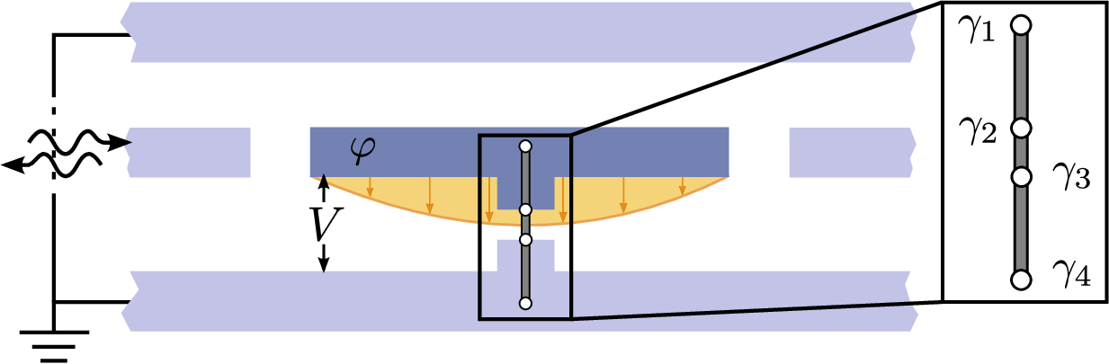
In this work, we want to employ the fractional Josephson radiation in order to implement a readout scheme for Majorana qubits. Instead of tuning the microwave cavity on resonance, we envision a setup in the dispersive regime allowing for a quantum nondemolition measurement. As the fractional Josephson radiation arises from single-electron transport due to the presence of MZMs, it allows for a direct readout of the Majorana qubit without involving intermediate interference steps. Coupling of the readout device to the Majorana qubit can be turned on and off at will via control of the external bias voltage.

In Sec. II we briefly introduce and review the coupling mechanism that leads to fractional Josephson radiation. We continue by introducing the effective model for a dispersive readout in Sec. III. We then study the susceptibility of the system to coherent radiation introduced by coupling the cavity to a transmission line resonator (Sec. IV). Finally in Sec. V, we compute the measurement times for a homodyne measurement scheme as well as for an intensity measurement showing that both methods profit from phase coherence. While this is always the case for the homodyne measurement, in the present situation, the MZMs lead to squeezing of the radiation, thereby also rendering the intensity measurement phase-sensitive.

A prominent way to emulate a topological superconductor in order to create MZMs is to employ nanowires having strong spin-orbit interaction in combination with an external magnetic field as well as proximity-induced Cooper pairing [7, 6]. In its topological phase, the nanowire hosts a pair of MZMs at its ends. Being zero energy modes of superconductors, MZMs are characterized by quasiparticle operators that are Hermitian, $\gamma_{j}=\gamma_{j}^{\dagger}$, and fulfill the Clifford algebra $\{\gamma_{j},\gamma_{k}\}=2\delta_{jk}$. In a superconductor, the fermion number is strongly fluctuating, and only the fermion parity $\mathcal{P}=\pm 1=(-1)^{N}$, with $N$ the total number of fermions, remains a good quantum number. In a one-dimensional topological superconductor, one can also define the fermion parity of a topological section as the product of the two Majorana end mode operators [4]. As the total fermion parity in a closed system is conserved, a qubit can only be realized in a system having two topological segments and thus four Majorana zero modes $\gamma_{1},\gamma_{2},\gamma_{3},\gamma_{4}$. Denoting the fermion parities of the segment between $\gamma_{1}$ and $\gamma_{2}$ ($\gamma_{3}$ and $\gamma_{4}$) by $\mathcal{P}_{12}=i\gamma_{1}\gamma_{2}$ ($\mathcal{P}_{34}=i\gamma_{3}\gamma_{4}$), the ground-state manifold is spanned by the states $|11\rangle$, $|\bar{1}1\rangle$, $|1\bar{1}\rangle$, and $|\bar{1}\bar{1}\rangle$, with $\mathcal{P}_{x}|p_{12}p_{34}\rangle=p_{x}|p_{12}p_{34}\rangle$, $p_{x}=\pm 1$, $x\in\{12,34\}$. The states $|11\rangle$, $|\bar{1}\bar{1}\rangle$ are characterized by an even number of fermions having the parity $\mathcal{P}=\mathcal{P}_{12}\mathcal{P}_{34}=1$, whereas the states with an odd number of fermionic particles $|1\bar{1}\rangle,|1\bar{1}\rangle$ have parity $\mathcal{P}=-1$ [26]. Most importantly, keeping the total fermion parity fixed, the MZMs form a two-level system (Majorana qubit) with the two states $|p_{12},\mathcal{P}p_{12}\rangle$ distinguished by $p_{12}=\pm 1$. The Pauli operators for the Majorana qubit are accordingly given by $\sigma_{z}=\mathcal{P}_{12}=i\gamma_{1}\gamma_{2}$ and $\sigma_{x}=i\gamma_{2}\gamma_{3}$ [8].

A single segment of a topological superconductor interrupted by a tunneling junction (a Majorana Josephson junction), such as that formed, for example, by a semiconducting nanowire bridging two superconductors, is a natural place to realize four MZMs; see Fig. 1. Two MZMs are situated at the ends of the nanowire, while two additional ones are formed on either side of the tunnel junction with the overlap tunable by the phase difference across the junction [27]. A distinctive feature of such a Majorana Josephson junction is the ability to coherently transport single electrons (and not only Cooper pairs) between the two superconductors [4, 28]. Such an event changes the fermion parity on either side of the wire and thus acts like a $\sigma_{x}$ on the Majorana qubit.

In the following, we consider the situation in which such a Majorana Josephson junction is embedded in a strip line resonator and coupled to its resonator modes via a dipole interaction Hamiltonian. Hence the system can be described by the total Hamiltonian

The first term $H_{0}=\frac{1}{2}\hbar\delta_{\mathcal{P}}\sigma_{z}$ arises due to finite overlap amplitudes of the MZMs on each wire [20]. This results in a small energy splitting $\hbar\delta_{\mathcal{P}}$ whose value in principle depends on the total fermion parity $\mathcal{P}$. The strip-line resonator with the resonance frequency $\omega_{c}$ is described by the Hamiltonian $H_{c}=\hbar\omega_{c}a^{\dagger}a$, with $a$ the annihilation operators of the cavity mode fulfilling the canonical commutation relation $[a,a^{\dagger}]=1$. Applying a voltage bias to the Majorana Josephson junction allows for single electron transfer that is accompanied by the emission/absorption of photons carrying the residual energy of the transition. The interaction of the Majorana Josephson junction with the electromagnetic environment is given by the dipole Hamiltonian [20]

here, $\varphi(t)$ is the superconducting phase difference across the junction, which is related to the voltage by $V=\hbar\dot{\varphi}/2e$. The voltage consists of two parts $V=V_{0}+V_{\text{ac}}$, with $V_{0}$ the dc voltage bias and a part due to the cavity field $V_{\text{ac}}=V_{\text{zp}}(a+a^{\dagger})$, which determines the light-matter interaction constant $g\simeq eV_{\text{zp}}/\hbar$. Here the strength of the vacuum fluctuations, $V_{\text{zp}}=(\hbar\omega_{c}/C)^{1/2}$, of the cavity is given by its total capacitance $C$ to ground. The physical significance of $\sigma_{x}$ is to implement the parity changes on either side, and $a^{({\dagger})}$ refers to the absorption (emission) of a photon. For the sake of implementing a qubit readout via microwave radiation, a superconducting transmission line is capacitively coupled to the cavity acting as a bus for the information to be read out; see Fig. 1.

As explained below, the measurement setup will be active when the dc voltage has a value $V_{0}\approx\hbar\omega_{c}/e$. Without the applied dc bias voltage, the superconducting phase difference $\varphi$ is constant up to quantum fluctuations due to the oscillator. Thus in this case, the first factor in Eq. (2) is almost constant and the second term becomes ineffective as emission or absorption of a photon requires the energy $\hbar\omega_{c}$. Tuning the dc voltage close to the value $\hbar\omega_{c}/e$ leads to the superconducting phase difference of the form

where we have introduced the Josephson frequency $\omega_{\scriptscriptstyle\rm J}=2eV_{0}/\hbar$ and the initial phase difference $\varphi_{0}$. The last term originates from the cavity mode and is given by $\varphi_{\text{ac}}=(2eV_{\text{zp}}/\hbar\omega_{c})\,i(a-a^{\dagger})$ since $\varphi_{\text{ac}}$ and $V_{\text{ac}}$ are canonically conjugate variables [29]. Its magnitude can be estimated as $\varphi_{\text{ac}}\simeq n^{1/2}eV_{\text{zp}}/\hbar\omega_{c}=(ne^{2}/\hbar\omega_{c}C)^{1/2}$, where $n$ denotes the number of photons in the cavity. In the following, we assume that the capacity is large enough such that $\omega_{c}C\gg ne^{2}/\hbar$, which corresponds to weak coupling ($n^{1/2}g\ll\omega_{c}$) [30]. As a result, we can approximately set $\varphi(t)=\varphi_{0}+\omega_{\scriptscriptstyle\rm J}t$. The combined dynamics of the Majorana qubit and the cavity is described by Hamiltonian (1), which is driven at half of the Josephson frequency due to the time-dependent superconducting phase in (3). By going to the interaction picture with respect to the Hamiltonian $H=\frac{1}{2}\hbar\omega_{{\scriptscriptstyle\rm J}}a^{\dagger}a$, the time evolution is determined by slowly varying variables $\tilde{a}=e^{i\omega_{\scriptscriptstyle\rm J}t/2}a$ corresponding to operators in a rotating frame. By neglecting off-resonant contributions, which appear as fast oscillating terms in the rotating frame, the Hamiltonian (1) maps to the time-independent quantum Rabi problem

where $\Omega=\omega_{c}-\omega_{{\scriptscriptstyle\rm J}}/2\ll\omega_{c}$ is the detuned frequency in the rotating frame [31]. In the following, we are interested in the regime of large detuning $\Omega\gg g,\delta_{\mathcal{P}}$ that is characterized by weak exchange of energy between the qubit and the cavity, therefore called the dispersive regime [33]. In this case, perturbation theory in the small parameter $g/\Omega$ is a well-controlled approximation as long as the number of photons $n$ in the cavity does not exceed the critical value $\Omega^{2}/g^{2}$. Using the technique of Schrieffer-Wolff transformation, we obtain the effective Hamiltonian

up to second order in $g/\Omega$. Due to virtual processes, the interaction shifts the cavity frequency and furthermore introduces the anomalous (quadrature squeezing) terms $\propto\tilde{a}^{2},\tilde{a}^{\dagger}{}^{2}$ which arise due to counter-rotating terms of the transversal coupling [34]. Note that the frequency shift as well as the squeezing amplitude are determined by the parameter $\chi=-2g^{2}\delta_{\mathcal{P}}/\Omega^{2}\ll\Omega$. Most importantly, both effects depend on the qubit state $\sigma_{z}$. To simplify the notation, we introduce the shifted cavity frequency $\tilde{\Omega}=\Omega+\chi\sigma_{z}$ with a small shift compared to the bare frequency $\Omega$. Therefore, the qubit state can be extracted by detecting the relative cavity shift $\pm\chi$ with respect to the undressed cavity frequency. For the case of homodyne detection, which we will discuss below, the measurement will be due to the first term of Eq. (5). On the contrary, for the intensity measurement, the last term will dominate.

The measurement of the Majorana qubit is performed by observing the shift in the cavity frequency, cf. (5), by probing the cavity via the transmission line. We want to take into account that the detector is not ideal in the sense that it does not capture every photon. For that purpose, we couple the resonator to two independent waveguides ($j\in\{1,2\}$), with the idea that the photons in the waveguide with $j=1$ are measured while the other photons are lost. The transmission lines are modeled by the Hamiltonian

with operators $b_{j}^{\dagger}(\omega),b^{\vphantom{\dagger}}_{j}(\omega)$ creating and annihilating microwave photons at the frequency $\omega$ fulfilling the commutation relation $[b^{\vphantom{\dagger}}_{j}(\omega),b^{\dagger}_{k}(\omega^{\prime})]=2\pi\delta_{jk}\delta(\omega-\omega^{\prime})$. The cavity field is coupled to the waveguides by the Hamiltonian

here, the coupling parameters $\kappa_{j}>0$ denote the decay rate of the cavity photons in the $j$-th transmission line. In the following, we will introduce the efficiency $\eta=\kappa_{1}/(\kappa_{1}+\kappa_{2})$ of the detector which denotes the fraction of detected photons. Neglecting spin-flip errors induced by off-resonant interaction of the qubit with the radiation [35], the combined qubit-cavity Hamiltonian $H$ commutes with $\sigma_{z}$ rendering the measurement to be a quantum nondemolition measurement. In this case, the interaction of the resonator with the transmission lines can be described by the quantum Langevin equations [32]

where the input field, defined as

satisfies the commutation relation $[\tilde{a}^{\vphantom{\dagger}}_{\text{in},j}(t),\tilde{a}^{\dagger}_{\text{in},k}(t^{\prime})]=\delta_{jk}\delta(t-t^{\prime})$. The output field is then given by the boundary condition $\tilde{a}_{\rm out,1}(t)=\tilde{a}_{\rm in,1}(t)+\kappa_{1}^{1/2}\tilde{a}(t)$ at the interface to the transmission line 1. The stochastic differential equations (8) can be solved for $\tilde{a}$ by going to frequency space with $\tilde{a}(\nu)=\int\!dt\,e^{i\nu t}\tilde{a}(t)$. The solution is given by the linear relation

between the input and the output fields. In our case, the annihilation operator of the output field is a coherent superposition of annihilation as well as creation operators of the input field. This can be traced back to the anomalous terms in (5). All the relevant information about the scattering of microwaves is encoded into the functions

where $\kappa=\kappa_{1}+\kappa_{2}$ is the total line width of the cavity. Note that they satisfy the identity $\sum_{j}(|u_{j}|^{2}-|v_{j}|^{2})=1$ which translates the canonical commutation relation from $\tilde{a}_{\text{in}}$ to $\tilde{a}_{\text{out}}$.

In the following, we will only consider the situation where the resonator is fed by a coherent state at frequency $\nu_{\text{in}}$ with $\langle\tilde{a}_{\text{in,1}}\rangle=e^{-i\nu_{\text{in}}t}\alpha_{\text{in}}$. For the second transmission line, we take the vacuum state as an input state that is valid in the low temperature limit at temperatures $T\ll\hbar\omega_{c}/k_{B}$. The radiation reflected back into the first transmission line, which will be subsequently measured, is characterized by its mean output signal

as well as by the correlation functions

here and below, the double brackets denote the (co-)variance defined as $\langle\langle AB\rangle\rangle=\langle AB\rangle-\langle A\rangle\langle B\rangle$. The squeezing term of Eq. (5) leads to the fact that both correlators in (13) are nonzero.

The qubit readout proceeds via the measurement of the ac voltage component $\propto a_{\rm out,1}$ that is reflected back from the cavity into the transmission line 1. As the ac voltage component oscillates at microwave frequencies, the signal frequency needs to be downconverted, which can be achieved by means of a homodyne measurement technique as well as by measuring the intensity which is the squared modulus of the voltage. Both schemes will be discussed in the following. To keep the discussion simple, we will discuss only the case in which the frequency of the input signal is given by $\nu_{\rm in}=\Omega+\chi$, i.e, it is on resonance with the cavity given that the qubit is in the state $\sigma_{z}=1$.

We have demonstrated how the embedding of a semiconducting nanowire bridging two superconductors in a microwave cavity can be utilized for the measurement of the Majorana qubit due to the four MZMs at the ends and the interface. The measurement proceeds by probing the transmission lines capacitively coupled to the cavity. In the dispersive regime of large qubit cavity detuning, the system implements a quantum nondemolition measurement. We have shown that the dispersive frequency shift can be either detected by a homodyne or alternatively by an intensity measurement. Although the intensity measurement contains an unusually large amount of coherence, it turns out not to be sufficient in order to compete with the dephasing time of the qubit. In contrast, with the homodyne measurement technique one is even able to push the measurement time towards the quantum limit. Thus, the microwave homodyne readout of the Majorana qubit promises to be a new scheme having the main advantages of providing a mechanism directly coupling microwave radiation to the topological qubit. Furthermore, the readout process can be turned on and off at will by simply changing the dc bias voltage.

We acknowledge financial support from the Alexander von Humboldt foundation.

References

- [1] A. Yu. Kitaev, Ann. Phys. (NY) 303, 2 (2003).
- [2] C. Nayak, S. H. Simon, A. Stern, M. Freedman, and S. Das Sarma, Rev. Mod. Phys. 80, 1083 (2008).
- [3] S. Das Sarma, M. Freedman, and C. Nayak, Phys. Rev. Lett. 94, 166802 (2005).
- [4] A. Yu. Kitaev, Phys.-Usp. 44 (suppl.), 131 (2001).
- [5] D. A. Ivanov, Phys. Rev. Lett. 86, 268 (2001).
- [6] R. M. Lutchyn, J. D. Sau, and S. Das Sarma, Phys. Rev. Lett. 105, 077001 (2010).
- [7] Y. Oreg, G. Refael, and F. von Oppen, Phys. Rev. Lett. 105, 177002 (2010).
- [8] C. W. J. Beenakker, Annu. Rev. Con. Mat. Phys. 4, 113 (2013).
- [9] J. Alicea, Rep. Prog. Phys. 75, 076501 (2012).
- [10] M. Leijnse and K. Flensberg, Semicond. Sci. Technol. 27, 124003 (2012).
- [11] V. Mourik, K. Zuo, S. M. Frolov, S. R. Plissard, E. P. A. M. Bakkers, and L. P. Kouwenhoven, Science 336, 1003 (2012).
- [12] A. Stern and B. I. Halperin, Phys. Rev. Lett. 96, 016802 (2006).
- [13] P. Bonderson, A. Kitaev, and K. Shtengel, Phys. Rev. Lett. 96, 016803 (2006).
- [14] F. Hassler, A. R. Akhmerov, C.-Y. Hou, and C. W. J. Beenakker, New J. Phys. 12, 125002 (2010).
- [15] J. D. Sau, S. Tewari, and S. Das Sarma, Phys. Rev. B 84, 085109 (2011).
- [16] F. Hassler, A. R. Akhmerov, and C. W. J. Beenakker, New J. Phys. 13, 095004 (2011).
- [17] D. Pekker, C.-Y. Hou, V. E. Manucharyan, and E. Demler, Phys. Rev. Lett. 111, 107007 (2013).
- [18] M. Trif and Ya. Tserkovnyak, Phys. Rev. Lett. 109, 257002 (2012).
- [19] A. Cottet, T. Kontos, and B. Douçot, Phys. Rev. B 88, 195415 (2013).
- [20] C. Ohm and F. Hassler, New J. Phys. 16, 015009 (2014).
- [21] T. L. Schmidt, A. Nunnenkamp, and C. Bruder, Phys. Rev. Lett. 110, 107006 (2013).
- [22] T. L. Schmidt, A. Nunnenkamp, and C. Bruder, New J. Phys. 15, 025043 (2013).
- [23] E. Ginossar and E. Grosfeld, Nature Commun. 5 (2014).
- [24] K. Yavilberg, E. Ginossar and E. Grosfeld, arXiv:1411.5699 (2014).
- [25] F. Domínguez, F. Hassler, and G. Platero, Phys. Rev. B 86, 140503(R) (2012).
- [26] We introduce the shorthand notation .
- [27] L. Fu and C. L. Kane, Phys. Rev. Lett. 100, 096407 (2008).
- [28] L. Fu and C. L. Kane, Phys. Rev. B 79, 161408 (2009).
- [29] The operator corresponding to the classical variable is given by in the Schrödinger picture.
- [30] Later, we will see that we even need to require that .
- [31] Note that contrary to the conventional case [32] due to the driving with a bias voltage the problem does not map to the Jaynes-Cummings problem in the rotating frame.
- [32] C. W. Gardiner and P. Zoller, Quantum Noise (Springer-Verlag Berlin Heidelberg, 2010).
- [33] M. Boissonneault, J. M. Gambetta, and A. Blais, Phys. Rev. A 79, 013819 (2009).
- [34] D. Zueco, G. M. Reuther, S. Kohler, and P. Hänggi, Phys. Rev. A 80, 033846 (2009).
- [35] In the dispersive frame also spin-flip terms are induced. These contributions can be regarded to be small as they only appear in first order of .
- [36] D. Rainis and D. Loss, Phys. Rev. B 85, 174533 (2012).
- [37] J. C. Budich, S. Walter, and B. Trauzettel, Phys. Rev. B 85, 121405 (2012).
- [38] M. Houzet, J. S. Meyer, D. M. Badiane, and L. I. Glazman Pys. Rev. Lett. 111, 046401 (2013)
- [39] F. Konschelle and F. Hassler, Phys. Rev. B 88, 075431 (2013).
- [40] M. Cheng, R. M. Lutchyn, and S. Das Sarma, Phys. Rev. B 85, 165124 (2012).
- [41] M. J. Schmidt, D. Rainis, and D. Loss, Phys. Rev. B 86, 085414 (2012).