Off-Shell Higgs Coupling Measurements in BSM scenarios
Abstract
Proposals of measuring the off-shell Higgs contributions and first measurements at the LHC have electrified the Higgs phenomenology community for two reasons: Firstly, probing interactions at high invariant masses and momentum transfers is intrinsically sensitive to new physics beyond the Standard Model, irrespective of a resonant or non-resonant character of a particular BSM scenario. Secondly, under specific assumptions a class of models exists for which the off-shell coupling measurement together with a measurement of the on-shell signal strength can be re-interpreted in terms of a bound on the total Higgs boson width. In this paper, we provide a first step towards a classification of the models for which a total width measurement is viable and we discuss examples of BSM models for which the off-shell coupling measurement can be important in either constraining or even discovering new physics in the upcoming LHC runs. Specifically, we discuss the quantitative impact of the presence of dimension six operators on the (de)correlation of Higgs on- and off-shell regions keeping track of all interference effects. We furthermore investigate off-shell measurements in a wider context of new (non-)resonant physics in Higgs portal scenarios and the MSSM.
I Introduction
The Higgs discovery in 2012 [1, 2] with subsequent (rather inclusive) measurements performed in agreement with the Standard Model (SM) hypothesis [3, 4] highlight the necessity to establish new Higgs physics-related search and analysis strategies that are sensitive to beyond the SM (BSM) interactions. In a phenomenological bottom-up approach the LHC’s sensitivity reach can be used to classify potential BSM physics, which we can loosely categorize models into four classes:
| (i) light hidden degrees of freedom, (ii) new degrees of freedom in the sub-TeV that induce non-resonant thresholds, (iii) resonant TeV scale degrees of freedom with parametrically suppressed production cross sections, (iv) new degrees of freedom in the multi-TeV range that can be probed in the energetic tail region of the 13 and 14 TeV options, or might even lie outside the energetic coverage of the LHC. | (1) |
The analysis strategies with which the LHC multi-purpose experiments can look for an individual category above typically build upon assumptions about the remaining three. These assumptions need to be specified in order for the result to have potential interpretation beyond the limitations of a certain specified scenario.
For example, if we deal with a large hierarchy of physics scales as in case (iv), we can rely on effective theory methods to set limits on the presence of new scale-separated dynamics. A well-motivated approach in light of electroweak precision measurements and current Higgs analyses is to extend the renormalizable SM Lagrangian by dimension six operators [5, 6, 7, 8, 9, 10, 11], which parametrize the leading order corrections of SM dynamics in the presence of new heavy states model-independently.
Given that the LHC machine marginalizes over a vast partonic energy range, the described effective field theory (EFT) methods are not applicable in cases (i)-(iii), for which new resonant dynamics is resolved; we cannot trust an EFT formulation in the presence of thresholds. In these cases we have to rely on agreed benchmark scenarios to make the interpretation of a limit setting exercise transparent.

In general, the standard analysis approach to BSM scenarios that fall into categories (ii)-(iv) focuses on large invariant masses and large momentum transfers. However, it is intriguing that a correlation of the low and high invariant mass measurements also allows us to constrain scenarios of type (i). An important analysis that has received a lot of attention from both the theoretical and the experimental community in this regard is the Higgs width measurement in as introduced by Caola and Melnikov [12]. Assuming the SM spectrum and neglecting renormalizability issues that arise when we employ the -language of recent Higgs coupling measurements [13], the proposed strategy exploits non-decoupling of the top loop contributing to (directly related to the top mass’ generation via the Higgs mechanism) and decoupling of the Higgs width parameter for large invariant masses to formulate a constraint on the Higgs width:
| (2a) | |||||
| (2b) | |||||
where is the partonic level center of mass energy and , where is the coupling in the SM and parametrizes BSM effects. Here, For simplicity, here we only consider gluon fusion, the dominant production mechanism. “Off-shell” typically means GeV due to a maximized ratio of Higgs-induced vs. continuum production as a consequence of the top threshold.
If we have , yet still a SM value for the signal strength , we need to have . If we consider an extrapolation of the on-shell region to the off-shell region based on the SM Feynman graph templates depicted in Fig. 1, we can understand a constraint on as a constraint on as a consistency check: In a well-defined QFT framework such as the SM, a particle width is a consequence of the interactions and degrees of freedom as specified in the Lagrangian density. E.g. by extending the SM with dynamics that induce an invisible partial Higgs decay width, there is no additional information in the off-shell measurement when combined with the on-shell signal strength. It is important to note that if we observe an excess in in the future, then this will not be a manifestation of . Instead we will necessarily have to understand this as a observation of physics beyond the SM, which might but does not need to be in relation to the Higgs boson.
A quantitatively correct estimate of important interference effects that shape have been provided in Refs. [14, 15, 16] (see also [17] for a related discussion of ). These interference effects are an immediate consequence of a well-behaved electroweak sector in the sub-TeV range in terms of renormalizability and, hence, unitarity [18, 19]. While they remain calculable in electroweak leading order Monte Carlo programs [14, 15], they are not theoretically well-defined, unless we assume a specific BSM scenario or invoke EFT methods. For a discussion on the unitarity constraints on the different Wilson coefficients see [20].
Both ATLAS and CMS have performed the outlined measurement with the 8 TeV data set in the meantime [21, 22]. The importance of high invariant mass measurements in this particular channel in a wider context has been discussed in Refs. [23, 24, 18, 25, 26]
In the particular case of , we can classify models according to their effect in the on-shell and off-shell phase space regions. We can identify four regions depending on the measured value of , which can provide a strong hint for new physics in the above scenarios (ii)-(iv):
| 1. and , 2. and , 3. and , 4. and . | (3) |
We can write a generalized version of Eq. (2b) that also reflects (non-)resonant BSM effects by writing the general amplitude
| (4) |
from which we may compute by folding with parton distribution functions and the phase space weight. For -induced production we can formulate a similar amplitude
| (5) |
which can impact the boson pair phenomenology on top of the -induced channels. Hence, for the differential off-shell cross section we find .
Resonant scenarios, such as new scalars and vectors are in agreement with the generalized Landau-Yang theorem [27] have been studied in detail [28]. Non-resonant new interactions involving light quarks, e.g. in a dimension six operator extension of the SM, are typically constrained.
For all models that fall into the classification 1. we are allowed to re-interpret the off-shell measurement as a constraint on the Higgs width bearing in mind theoretical shortcomings when parameters are varied inconsistently; the uncertainty of a measurement of and the on-shell signal strength combine to a constraint on . Assuming new physics exists, such a constraint makes strong assumptions about potential cancellations among or absence of the new physics couplings in the off-shell region. In particular because the effective couplings are phase space dependent and can affect the differential distribution beyond a simple rescaling. A concrete example of this class of models is the general dimension six extension of the SM Higgs sector with a Higgs portal to provide an invisible partial decay width . If we are in the limit of vanishing dimension six Wilson coefficients , new EFT physics contributions with new physics scale in the on- and off-shell regions are parametrically suppressed and the dominant unconstrained direction in this measurement is . Note that there can be cancellations in the high invariant mass region among different dimension six coefficients, so the constraint formulated on requires .
For the second scenario a re-interpretation in terms of a width measurement is generally not valid. Here, the SM off-shell distribution is recovered while the on-shell signal strength is unity due to a cancellation between the modified Higgs width and the on-shell coupling modification. A toy-model example has been discussed in [18].
From a phenomenological point of view, scenarios 3. and 4. are of great interest, in particular because SM-like signal strength measurements alone do typically not provide enough information to rule out models conclusively. Most concrete realizations of BSM physics predict new physics at high energies as a unitarity-related compensator for modifications of on-shell coupling strengths. “Off-shell” measurements are therefore prime candidates to look for deviations from the Standard Model in the sense that they will be sensitive to new resonances [29] and will have strong implications for BSM physics in general.
The aim of this work is to provide a survey of the reach of the validity of the Higgs width interpretation. Since modifications of the Higgs width do imply physics beyond the SM, the Higgs width interpretation can be reconciled with new physics effects in the channel. This allows us to make contact to concrete phenomenological realizations using the above categorization. New degrees of freedom as introduced in the beginning of this section that give rise to new contributions following Eq. (4).
We focus on -induced production throughout. We will first discuss light non-resonant degrees of freedom and their potential impact on the distributions with the help of toy models that we generalize to the (N)MSSM in Sec. III.1. Assuming a scale separation between new resonant phenomena and the probed energy scales in we discuss high invariant mass boson pair production in a general dimension six extension of the SM in Sec. III.2 before we consider resonant phenomena in Sec. IV. In particular, our calculation includes all interference effects (at leading order) of in all of these scenarios. Our discussions and findings straightforwardly apply to the channel which is, due to custodial symmetry, closely related to the final state.
II A note on the Monte Carlo Implementation
The numerical calculations in this paper have been obtained with a customized version of Vbfnlo [30], that employs FeynArts/FormCalc/LoopTools [31] tool chain for the full final state (see Fig. 1). We neglect QED contributions throughout; they are known to be negligible especially for the high phase space region where both bosons can be fully reconstructed. Our implementation is detailed in [18] and has been validated against the SM results of [15]. We include bottom quark contributions to the Higgs diagrams in Fig. 1, these can become relevant in the MSSM at large . The effective theory implementation has been checked for consistency against existing implementations [32] (normalizations and Feynman rules) based on FeynRules [33]. The phase space integration has been validated against the results of [15]. Throughout we apply inclusive cuts
| (6) |
where is the angular separation between any two leptons, and are the lepton rapidity and transverse momentum respectively, and focus on LHC collisions at 13 TeV.
III Non-Resonant BSM Physics
Qualitative discussion of BSM contributions
To zoom in on the classes of models where a width interpretation is valid we note that, assuming peculiar cancellation effects among the couplings are absent, the coupling which has to be present and affects the on-shell and off-shell region in the least constraint way is the coupling. Further, crucial to a width interpretation in (3) is a strict correlation of the on- and off-shell regions which can be broken if light degrees of freedom are present following our classification in (1). If these light states carry color charge and obtain a mass that is unrelated to the electroweak vacuum, they will decouple quickly for , although they can provide a notable contribution to the Higgs on-shell region [18]. Inspired by the assumption that [22], parametrically this correlation requirement for is captured by the complex double ratio
| (7) |
If independent of within experimental uncertainties, the off-shell coupling measurement can be re-interpreted in terms of a width measurement. Note, has to be imposed as an additional requirement to ensure consistency with experimental measurements. Scenarios 1. and 4. can satisfy this condition, however, if a significant deviation of the Standard Model prediction is observed in the off-shell regime reinterpreting this observation in terms of a non-SM-like width for the Higgs resonance is likely to be of minor interest compared to the discovery of new physics.
The (de)correlation between the on- and off-shell measurements can be demonstrated by the following simple toy examples: we consider a scalar with mass , a fermion with mass as extra particles added to the SM spectrum. We allow these states to couple to the Higgs boson with interactions
| (8) |
where GeV. The coefficients parameterize the deviation from the SM-like case where the entire particle mass is originated from the Higgs mechanism with one doublet. In addition, we also take into account the contribution of the dimension six operator .


The amplitude relative to the SM one is given by
| (9) |
where are the scalar and fermion loop functions [34] and . for the fundamental representation of and the indices run over all scalars and fermions (i.e. including the SM fermions). We also include an effective interaction as the last term in Eq. (9) that we will discuss further in Sec. III.2 below.
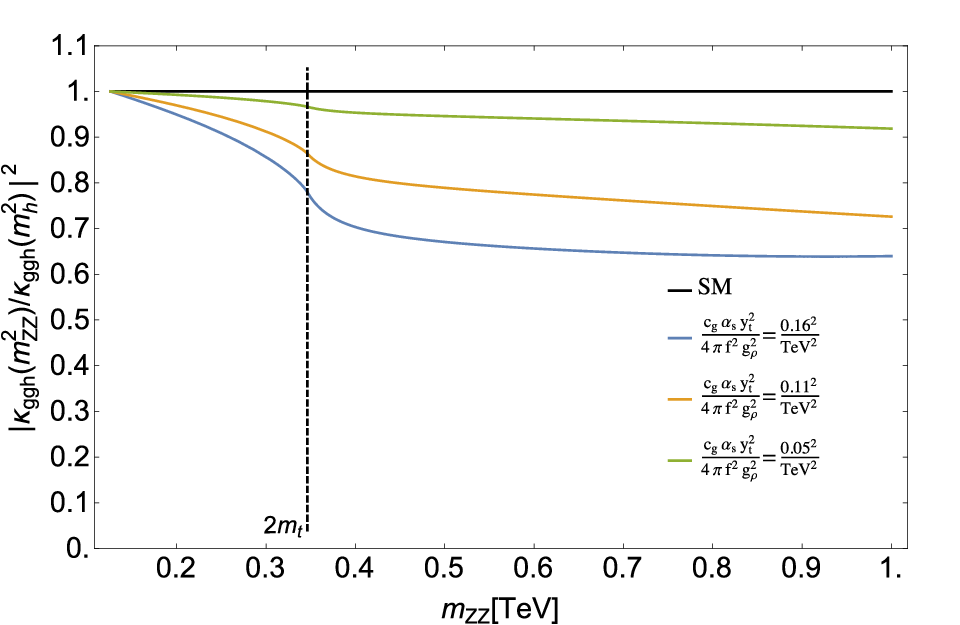
In Figs. 2 and 3 we show the ratio between the off- and on-shell differential couplings, , as a function of the invariant mass. We consider the case of a color-triplet representation and masses of GeV with . Depending on the size and sign of the BSM couplings, (a) we can get a cancellation or an enhancement between the SM and the new physics contributions for the subamplitude that follows from Fig. 1 (a). If these effects are large we cannot extrapolate the off-shell region to the on-shell region unless we know the specifics of the interaction and the particle mass. However, if the new physics scenario is such that it uniformly converges to the SM case we can understand the measurement as a probe of the Higgs width. The dimension six extension of the SM provides an example of such a scenario as already mentioned in the introduction and shown in Fig. 4. There we show the impact of an effective operator with a Wilson coefficient of
| (10) |
How realistic is an extension including light degrees of freedom? In the MSSM, a light scalar can be incorporated as the super partner of the top. For non-degenerate squark masses, current exclusion limits for stop searches are depending on several assumptions, e.g. the mass of the lightest supersymmetric particle [35, 36]. Thus, excluding stops with masses in the 100 GeV range categorically is at the moment not possible.
III.1 Light Degrees of Freedom
The MSSM
As pointed out in the previous section, the MSSM is a candidate model that can include light scalar degrees of freedom. Furthermore, the final state will receive additional resonant contributions from the heavy Higgs partner of the MSSM Higgs sector. While those contributions are fully included in our implementation, we will discuss them in detail later in this paper.
To achieve a relatively large mass of GeV for the lightest CP-even Higgs boson , while maintaining a light stop, large -terms are necessary which in turn increase the chiral component of the stop-Higgs coupling** * Large -terms are constrained by vacuum stability requirements [37].. However, the Higgs mass constraint can be satisfied by introducing other degrees of freedom, e.g. as pursued in the NMSSM [38], and a large mass splitting of the two stops can be realized with large soft mass components or without inducing a large Higgs-stop coupling. Therefore, the limits we discuss in Sec.III can be realized in the (N)MSSM.

We do not delve into the details of non-minimal SUSY model-building, but we want to stress the crucial points that phenomenologically impact searches at large from a slightly different angle compared to the previous section: Since the stop contributions obtain a chiral component which can be large as a function of the MSSM parameters and [34], additional thresholds in diagrams of type Fig. 1 (a) can impact the high invariant mass tail [18]. We stress that limits on stops from direct searches highly depend on [35, 36], assuming prompt decays. Thus, probing stops via their contributions to loop-induced processes can allow to set limits in a less model-dependent way.
Eqs. (8) expressed in terms of Higgs-quark interactions in the MSSM yields the coefficients [34]
| (11) |
with being the ratio of the vacuum expectations and the neutral scalar mixing angle. For the stop it can be approximated by
| (12) |
where , and is the stop mixing angle with the trilinear coupling .
To understand the quantitative effects, we choose throughout and consider
| (i) | (13) | |||
| (ii) | (14) |
We assume degenerate soft-mass terms and vary such to obtain and . Hence, larger results in larger and therefore larger Higgs-stop couplings, see Eq. (12). The high invariant mass region in can become an efficient indirect probe of the existence of light stops provided a non-negligible Higgs-stop coupling. The latter is phenomenologically preferred to achieve the relatively large GeV.
We show the different distributions for those parameter choices in Fig. 5, keeping fixed. Constraints on low stop masses in this particular parameter range of the (N)MSSM can be formulated in the absence of a stop-induced threshold for . As demonstrated in Fig. 5, the effects quickly decouple with larger stop masses and smaller values of .
III.2 Effective Field Theory
Higgs effective field theory has gained a lot of attention in the past and recently [5, 6, 7, 8, 9, 9, 11] and there is a rich phenomenology of anomalous Higgs couplings in production. To keep our discussion as transparent as possible we will choose the convention of [8] in the following:
| (15) |
with . It is worth pointing out that the operator basis is completely identical to a general dimension six extension of the SM Higgs sector [7], and differs from it by a bias on the Wilson coefficients that can be motivated from an approximate shift symmetry related to the interpretation of the Higgs as pseudo-Nambu Goldstone boson [8]. This bias suppresses certain operators relative to others, and the differential cross section will mostly depend on a subset of Wilson coefficients for identically chosen coefficients in Eq. (15). In a particular BSM scenario this can or might not be true; we simply adopt the language of [8] to illustrate the quantitative impact of a highlighted set of dimension six operators, while our numerical implementation incorporates all operator structures of Eq. (15). We work with a canonically normalized and diagonalized particle spectrum that, after appropriate finite field and coupling renormalization, does not modify the continuum contribution (this has been checked numerically and analytically).


We do not consider dipole operators of the form which will impact the continuum production of and . New physics contributions to the latter processes need to be treated independently in a concrete experimental analysis and is beyond the scope of our work. For demonstration purposes we choose
| (16) |
and for the spectra of Fig. 6.
From Fig. 6, it becomes apparent that the high invariant mass region has an excellent sensitivity to the dimension six operators of Eq. (15). We have chosen a SM signal strength which selects a region in the space of Wilson coefficients [9]. This region can be further constrained by including complementary information from a measurement of region [23, 25, 26]. This allows us to formulate the Higgs width as a function of the relevant dimension six operator coefficients through correlating Eqs. (2a) and (2b). Note that operator mixing [40, 41] is anticipated to impact the phenomenology of this Lagrangian at the 10% level if scales are vastly separated [42, 43]. Hence, the comparison of on- and off-shell measurements is direct . If we invoke the operator coefficient bias and of Eq. (15) focus on a tree-level parameter , the dominant operator coefficients that are probed in the off-shell region are .
A targeted analysis of how far these parameters can be constrained at the LHC has been presented in Ref. [26]; a question that remains worth addressing in this context, however, is the impact of the off-shell measurement in comparison to Higgs measurements in other channels such as associated Higgs [44, 45] and Higgs+jet [46] production.
In the following we input the SM-like signal strengths in the channel since direct measurements in the latter channels are not available at 8 TeV. The signal distributions for a representative operator choice is given in Fig. 7 and we use eHdecay [9] to compute the modified branching ratios, inputing the the bigger Higgs width to achieve . The different thresholds and normalizations in Fig. 7 reflect the signal regions and selection efficiencies as documented in the literature [45, 47] due to -tagging, reconstruction and subjet techniques.
It should be noted that associated Higgs and Higgs+jet production are plagued with large backgrounds as opposed to the experimentally clean signature†† † For instance, a measurement of the off-shell cross section is already available with the 8 TeV data set although the inclusive signal cross section is significantly smaller compared to -associated and jet-associated Higgs production, the signal-to-background ratio in e.g. is of the order of 0.1 [47]. A measurement of the differential distributions as shown in Fig. 7 in these channels will be complicated: While the acceptance in the fully leptonic final state at large invariant four-lepton masses is close to unity [22, 21], the signal rates in associated and monojet production are vastly reduced (for details see e.g. [45] and [47]). Therefore, off-shell measurements in the channel will not only provide crucial information to limit the presence of higher dimensional operators but also provide complementary information, in particular due to a larger kinematically accessible phase space range.


IV Resonant BSM Physics
In contrast to the non-resonant physics scenarios discussed in the previous sections, we can imagine the off-shell measurement to be impacted by the presence of additional iso-singlet scalar resonances. To work in a consistent framework, we will focus on so-called Higgs portal scenarios [48] in the following, which directly link the presence of new scalar states to a universal Higgs coupling suppression. We focus on the minimal extension of the Higgs sector
| (17) |
If both the Higgs doublet and the extra singlet obtain a vacuum expectation value, the -induced linear mixing introduces a characteristic mixing angle to single Higgs phenomenology via rotating the Lagrangian eigenstates () to the mass eigenbasis ()‡‡ ‡ Multi-Higgs phenomenology can be vastly different [49].
| (18) |
Consequently, we have two mass states with a SM-like phenomenology; such models have been studied in detail and we refer the reader to the literature [50, 51, 49].


We focus on scenarios
| (19) | ||||
| (20) |
and keep the Higgs width identical to the SM (this could be facilitated by another portal interaction to light SM-singlet states). This will modify the on-shell Higgs phenomenology and we choose , which is within the limits as reported in latest coupling fits in the category (see e.g. [4]). This choice is also consistent with the non-observation of a heavy Higgs-like particle with a signal strength of of the SM expectation in a region where the narrow width approximation is valid (see e.g. recent searches by CMS [52]) and limits set by electroweak precision constraints; see also [53] for a detailed discussion of currently allowed parameter range, and [50] on constraints that can be obtained by measuring the heavy Higgs boson
Since the light Higgs width quickly decouples this choice is irrelevant for the phenomenology at high invariant mass. To keep our discussion transparent, we choose a trivial hidden sector phenomenology by using
| (21) |
in the following. The results for two representative choices of are shown in Fig. 8.
The structure in the “” signal results from a destructive interference of the Higgs diagrams in the intermediate region as a consequence of the propagator structure and will depend on how we formulate the Higgs width theoretically [54].§§ § A survey of dip structures in cross sections has been presented in Refs. [55, 56]. From a phenomenological perspective this structure is numerically irrelevant.
Apart from the obvious additional resonance, we do not find a notable deviation from the SM away from the Breit-Wigner “turn on” region . Away from all -channel particle thresholds, i.e. for invariant masses , the amplitude becomes highly resemblant to the SM amplitude as a consequence of the linear mixing: If we write the SM top-triangle subamplitude as and remove the boson polarization vectors, we have an amplitude
| (22) |
which is just the SM contribution evaluated at large . This qualitative argument is numerically validated for the full cross section in Fig. 9. The differential distribution approaches the SM distribution rather quickly, especially because consistency with the 125 GeV signal strength measurements and electroweak precision data [57] imposes a hierarchy .
Eq. (22) suggests that the more interesting parameter choice for modified interference effects at large invariant masses is a larger mixing. In this case, however, the Higgs on-shell phenomenology would vastly modified too. Larger values of also imply tension with electroweak precision data and direct search constraints, unless we give up the simplified model of Eq. (17). This is beyond the scope of this work. Quantitatively a larger mixing only shows a moderate increase for GeV (we include a maximum mixing angle to Fig. 9), which results from Breit-Wigner distribution of the state ; for maximal mixing this has a larger signal strength compared to the scenario.
In summary, we conclude that the basic arguments that have been used in the interpretation of SM measurements [14, 15, 16, 17, 21, 22] remain valid in this minimal resonant extension of the SM Higgs sector. Our analysis straightforwardly generalizes to the two Higgs doublet model [58] and the HDM [59].
V Summary and Conclusions
Measurements at large momentum transfers as a probe of non-decoupling off-shell Higgs contributions provide an excellent testing ground of various scenarios of BSM physics.
In this paper we have further examined the validity of the interpretation of off-shell measurements as a probe of the Higgs total width. In combination with a signal strength , we motivate the double ratio of Eq. (7) as guideline for when this interpretation is valid, namely within uncertainties.
Furthermore, measurements at large invariant masses in at the LHC run 2 will have significant impact on searches for BSM physics far beyond the interpretation in terms of the Higgs’ width. We have discussed a wide range of BSM scenarios as examples that highlight this fact. In particular, we have provided a quantitative analysis of the high invariant mass region of in the context of the MSSM, a general dimension six extension of the SM Higgs sector, and resonant phenomena within Higgs portal scenarios.
Generic to all BSM scenarios is the model-dependence of the off-shell region. If we observe an excess in the future in the high region, the interpretation of such an observation is not necessarily related to the Higgs but could be a general effect of the presence of new TeV-scale dynamics. In particular, the “off-shell signal strength” has no relation to on-shell Higgs properties such as the width or even Higgs couplings, unless imposed by a choice of a particular class of BSM scenarios such as Eq. (15). An example of that, which we have not discussed in further detail are electroweak magnetic operators or an additional broad and heavy boson, that can impact the -induced production channels in a way that is a priori unrelated to the Higgs sector.
Acknowledgements.
We thank Ian Low for suggesting a quantitative analysis of the interference effects in the portal-extended SM and Gilad Perez and Andreas Weiler for valuable discussions. CE is supported by the Institute for Particle Physics Phenomenology Associateship program. MS thanks the Aspen Center for Physics for hospitality while part of this work was completed. This work was supported in part by the National Science Foundation under Grant No. PHYS-1066293.References
- [1] G. Aad et al. [ATLAS Collaboration], Phys. Lett. B 716 (2012) 1.
- [2] S. Chatrchyan et al. [CMS Collaboration], Phys. Lett. B 716 (2012) 30.
- [3] A. Azatov, R. Contino and J. Galloway, JHEP 1204 (2012) 127. P. P. Giardino, K. Kannike, M. Raidal and A. Strumia, Phys. Lett. B 718 (2012) 469. J. Ellis and T. You, JHEP 1209 (2012) 123. J. R. Espinosa, C. Grojean, M. Muhlleitner and M. Trott, JHEP 1212 (2012) 045. D. Carmi, A. Falkowski, E. Kuflik, T. Volansky and J. Zupan, JHEP 1210, 196 (2012). T. Plehn and M. Rauch, Europhys. Lett. 100, 11002 (2012). T. Corbett, O. J. P. Eboli, J. Gonzalez-Fraile and M. C. Gonzalez-Garcia, Phys. Rev. D 87 (2013) 015022. E. Masso and V. Sanz, Phys. Rev. D 87 (2013) 3, 033001. A. Djouadi and G. Moreau, arXiv:1303.6591 [hep-ph]. P. Bechtle, S. Heinemeyer, O. Stal, T. Stefaniak and G. Weiglein, arXiv:1403.1582 [hep-ph].
- [4] The CMS collaboration, CMS-PAS-HIG-14-009. The ATLAS collaboration, ATLAS-CONF-2014-009, ATLAS-COM-CONF-2014-013.
- [5] K. Hagiwara, R. D. Peccei, D. Zeppenfeld and K. Hikasa, Nucl. Phys. B 282 (1987) 253.
- [6] W. Buchmuller and D. Wyler, Nucl. Phys. B 268, 621 (1986).
- [7] B. Grzadkowski, M. Iskrzynski, M. Misiak and J. Rosiek, JHEP 1010 (2010) 085.
- [8] G. F. Giudice, C. Grojean, A. Pomarol and R. Rattazzi, JHEP 0706 (2007) 045.
- [9] R. Contino, M. Ghezzi, C. Grojean, M. Muhlleitner and M. Spira, JHEP 1307 (2013) 035;
- [10] A. Pomarol and F. Riva, JHEP 1401 (2014) 151.
- [11] T. Corbett, O. J. P. Eboli, J. Gonzalez-Fraile and M. C. Gonzalez-Garcia, Phys. Rev. D 86 (2012) 075013. B. Dumont, S. Fichet and G. von Gersdorff, JHEP 1307 (2013) 065.
- [12] F. Caola and K. Melnikov, Phys. Rev. D 88 (2013) 054024.
- [13] S. Heinemeyer et al. [LHC Higgs Cross Section Working Group Collaboration], arXiv:1307.1347 [hep-ph].
- [14] N. Kauer and G. Passarino, JHEP 1208 (2012) 116. N. Kauer, JHEP 1312 (2013) 082. N. Kauer, Mod. Phys. Lett. A 28 (2013) 1330015.
- [15] J. M. Campbell, R. K. Ellis and C. Williams, JHEP 1404 (2014) 060. J. M. Campbell, R. K. Ellis and C. Williams, Phys. Rev. D 89 (2014) 053011. J. M. Campbell, R. K. Ellis, E. Furlan and R. Röntsch, arXiv:1409.1897 [hep-ph].
- [16] I. Moult and I. W. Stewart, arXiv:1405.5534 [hep-ph].
- [17] L. J. Dixon and Y. Li, Phys. Rev. Lett. 111 (2013) 111802. L. J. Dixon and M. S. Siu, Phys. Rev. Lett. 90 (2003) 252001. S. P. Martin, Phys. Rev. D 88 (2013) 1, 013004. S. P. Martin, Phys. Rev. D 86 (2012) 073016.
- [18] C. Englert and M. Spannowsky, Phys. Rev. D 90 (2014) 053003.
- [19] M. S. Chanowitz, M. A. Furman and I. Hinchliffe, Phys. Lett. B 78 (1978) 285. M. S. Chanowitz, M. A. Furman and I. Hinchliffe, Nucl. Phys. B 153 (1979) 402.
- [20] A. Biekoetter, A. Knochel, M. Kraemer, D. Liu and F. Riva, arXiv:1406.7320 [hep-ph].
- [21] The CMS collaboration, Phys. Lett. B 736 (2014) 64.
- [22] The ATLAS collaboration, ATLAS-CONF-2014-042.
- [23] B. Coleppa, T. Mandal and S. Mitra, arXiv:1401.4039 [hep-ph]. J. S. Gainer, J. Lykken, K. T. Matchev, S. Mrenna and M. Park, arXiv:1403.4951 [hep-ph]. B. Grinstein, C. W. Murphy and D. Pirtskhalava, JHEP 1310 (2013) 077.
- [24] Y. Chen, R. Harnik and R. Vega-Morales, arXiv:1404.1336 [hep-ph].
- [25] M. Ghezzi, G. Passarino and S. Uccirati, arXiv:1405.1925 [hep-ph]. I. Brivio, O. J. P. Eboli, M. B. Gavela, M. C. Gonzalez-Garcia, L. Merlo and S. Rigolin, arXiv:1405.5412 [hep-ph].
- [26] G. Cacciapaglia, A. Deandrea, G. D. La Rochelle and J. B. Flament, arXiv:1406.1757 [hep-ph]. A. Azatov, C. Grojean, A. Paul and E. Salvioni, arXiv:1406.6338 [hep-ph].
- [27] W. Y. Keung, I. Low and J. Shu, Phys. Rev. Lett. 101 (2008) 091802.
- [28] Y. Gao, A. V. Gritsan, Z. Guo, K. Melnikov, M. Schulze and N. V. Tran, Phys. Rev. D 81 (2010) 075022. C. Englert, C. Hackstein and M. Spannowsky, Phys. Rev. D 82 (2010) 114024. S. Bolognesi, Y. Gao, A. V. Gritsan, K. Melnikov, M. Schulze, N. V. Tran and A. Whitbeck, Phys. Rev. D 86 (2012) 095031. P. Artoisenet, P. de Aquino, F. Demartin, R. Frederix, S. Frixione, F. Maltoni, M. K. Mandal and P. Mathews et al., JHEP 1311 (2013) 043.
- [29] H. E. Logan, arXiv:1412.7577 [hep-ph]. E. Maina, arXiv:1501.02139 [hep-ph]. N. Kauer and C. O’Brien, arXiv:1502.04113 [hep-ph]. C. Englert, I. Low and M. Spannowsky, Phys. Rev. D 91 (2015) 7, 074029.
- [30] K. Arnold, M. Bahr, G. Bozzi, F. Campanario, C. Englert, T. Figy, N. Greiner and C. Hackstein et al., Comput. Phys. Commun. 180 (2009) 1661. J. Baglio, J. Bellm, F. Campanario, B. Feigl, J. Frank, T. Figy, M. Kerner and L. D. Ninh et al., arXiv:1404.3940 [hep-ph].
- [31] T. Hahn and M. Perez-Victoria, Comput. Phys. Commun. 118 (1999) 153. T. Hahn, Comput. Phys. Commun. 140 (2001) 418. T. Hahn, PoS ACAT 2010 (2010) 078.
- [32] A. Alloul, B. Fuks and V. Sanz, JHEP 1404 (2014) 110.
- [33] A. Alloul, N. D. Christensen, C. Degrande, C. Duhr and B. Fuks, Comput. Phys. Commun. 185 (2014) 2250.
- [34] A. Djouadi, Phys. Rept. 459 (2008) 1. M. Muhlleitner and M. Spira, Nucl. Phys. B 790 (2008) 1.
- [35] The ATLAS collaboration, JHEP 1409, 015 (2014), arXiv:1407.0583 [hep-ex], Phys. Rev. D 90, 052008 (2014).
- [36] The CMS collaboration, Eur. Phys. J. C 73, 2677 (2013), CMS-PAS-SUS-13-009.
- [37] M. Reece, New J. Phys. 15, 043003 (2013).
- [38] M. Maniatis, Int. J. Mod. Phys. A 25 (2010) 3505. U. Ellwanger, C. Hugonie and A. M. Teixeira, Phys. Rept. 496 (2010) 1.
- [39] M. E. Peskin and T. Takeuchi, Phys. Rev. Lett. 65 (1990) 964. M. E. Peskin and T. Takeuchi, Phys. Rev. D 46 (1992) 381.
- [40] E. E. Jenkins, A. V. Manohar and M. Trott, JHEP 1310 (2013) 087. E. E. Jenkins, A. V. Manohar and M. Trott, JHEP 1401 (2014) 035. R. Alonso, E. E. Jenkins, A. V. Manohar and M. Trott, JHEP 1404 (2014) 159.
- [41] J. Elias-Miro, J. R. Espinosa, E. Masso and A. Pomarol, JHEP 1311 (2013) 066.
- [42] C. Grojean, E. E. Jenkins, A. V. Manohar and M. Trott, JHEP 1304 (2013) 016.
- [43] C. Englert and M. Spannowsky, arXiv:1408.5147 [hep-ph].
- [44] J. M. Butterworth, A. R. Davison, M. Rubin and G. P. Salam, Phys. Rev. Lett. 100 (2008) 242001 [arXiv:0802.2470 [hep-ph]].
- [45] C. Englert, M. McCullough and M. Spannowsky, Phys. Rev. D 89 (2014) 1, 013013.
- [46] R. V. Harlander and T. Neumann, Phys. Rev. D 88 (2013) 074015. A. Banfi, A. Martin and V. Sanz, JHEP 1408 (2014) 053. C. Grojean, E. Salvioni, M. Schlaffer and A. Weiler, JHEP 1405, 022 (2014).
- [47] M. Schlaffer, M. Spannowsky, M. Takeuchi, A. Weiler and C. Wymant, Eur. Phys. J. C 74 (2014) 10, 3120. M. Buschmann, C. Englert, D. Goncalves, T. Plehn and M. Spannowsky, Phys. Rev. D 90 (2014) 1, 013010. M. Buschmann, D. Goncalves, S. Kuttimalai, M. Schonherr, F. Krauss and T. Plehn, arXiv:1410.5806 [hep-ph].
- [48] T. Binoth and J. J. van der Bij, Z. Phys. C 75 (1997) 17. R. Schabinger and J. D. Wells, Phys. Rev. D 72 (2005) 093007. B. Patt and F. Wilczek, hep-ph/0605188.
- [49] M. Bowen, Y. Cui and J. D. Wells, JHEP 0703 (2007) 036. C. Englert, J. Jaeckel, E. Re and M. Spannowsky, Phys. Rev. D 85 (2012) 035008. M. J. Dolan, C. Englert and M. Spannowsky, Phys. Rev. D 87 (2013) 5, 055002. C. Englert, J. Jaeckel, V. V. Khoze and M. Spannowsky, JHEP 1304 (2013) 060. M. Heikinheimo, A. Racioppi, M. Raidal, C. Spethmann and K. Tuominen, Mod. Phys. Lett. A 29 (2014) 1450077. S. Y. Choi, C. Englert and P. M. Zerwas, Eur. Phys. J. C 73 (2013) 2643. V. V. Khoze, C. McCabe and G. Ro, JHEP 1408 (2014) 026.
- [50] C. Englert, T. Plehn, D. Zerwas and P. M. Zerwas, Phys. Lett. B 703 (2011) 298.
- [51] E. Weihs and J. Zurita, JHEP 1202 (2012) 041. D. Bertolini and M. McCullough, JHEP 1212 (2012) 118. G. M. Pruna and T. Robens, Phys. Rev. D 88 (2013) 115012. R. Foot, A. Kobakhidze and R. R. Volkas, Phys. Rev. D 84 (2011) 095032.
- [52] S. Chatrchyan et al. [CMS Collaboration], Eur. Phys. J. C 73, 2469 (2013).
- [53] A. Falkowski, C. Gross and O. Lebedev, arXiv:1502.01361 [hep-ph].
- [54] M. H. Seymour, Phys. Lett. B 354 (1995) 409. S. Goria, G. Passarino and D. Rosco, Nucl. Phys. B 864 (2012) 530.
- [55] Y. Bai and W. Y. Keung, arXiv:1407.6355 [hep-ph].
- [56] S. Willenbrock and G. Valencia, Phys. Lett. B 259 (1991) 373; R. G. Stuart, Phys. Lett. B 262 (1991) 113; U. Baur and D. Zeppenfeld, Phys. Rev. Lett. 75 (1995) 1002.
- [57] M. Baak et al. [Gfitter Group Collaboration], Eur. Phys. J. C 74 (2014) 3046 [arXiv:1407.3792 [hep-ph]].
- [58] J. F. Gunion and H. E. Haber, Phys. Rev. D 67 (2003) 075019.
- [59] Y. Grossman, Nucl. Phys. B 426 (1994) 355.